1. Introduction
In this article, we use an expanded structure of the symmetric group over the set of permutations from to to develop a dependence detection procedure in bivariate random vectors. The procedure is based on identifying the longest non-decreasing subsequence (LNDSS) detected in the graph of the paired marginal ranks of the observations. It records the size of the subsequence and verifies the chances that it has to occur in the expanded space of under the assumption of independence between the variables. The procedure does not require assumptions about the type of the two random variables being tested, such as being both discrete, both continuous or a mixed structures (discrete-continuous).
When we face the challenge of deciding whether the independence between random variables can be discarded, it is necessary to establish the nature of the variables, whether they are continuous or discrete. For continuous random variables, we have several procedures, for example, Hoeffding’s test and those based on dependence’s coefficients (Spearman’s coefficient, Pearson’s coefficient, Kendall’s coefficient, etc.). Instead, for the discrete case, the options are few, the most popular is Pearson’s Chi-squared test. Also, the tests based on Kendall and Spearman coefficients going through corrections that consider ties can be used to test for independence between two discrete and ordinal variables (see [
1,
2]). In general, recommended for small sample sizes. Moreover, some derivations of the Chi-squared statistic have been projected to test independence between two nominal variables, as is the case of the Cramér’s
V statistic, see [
3].
The goal of this article is to show an independence test, developed from the notion of the LNDSS among the ranks of the observations, see [
4]. The main notion was introduced previously in [
5] with a different implementation from the one proposed in this paper. The alterations proposed in this paper aim to improve the procedure’s performance. This methodology works without limitation on the type of the two random variables being tested, which can be continuous/discrete.
The existence of ties in a dataset cast doubts about the use of matured tests for continuous variables, see, for instance, [
6] for a discussion on this issue. The use of procedures preconized for continuous random variables, in cases with repetitions in the observations due to the precision used to record the data, may have unforeseen consequences on the performance of the procedure. If the ties are eliminated, the use of asymptotic distributions can be compromised, if the ties are considered (by means of some correction), the control of type 1 and 2 errors can be put at risk (increasing the false positives/negatives of the procedure). Another frequent situation is when one of the variables is continuous, and the other is discrete. For some test of independence, problems may arise from this situation forcing the practitioner to apply some arbitrary data categorization. Under this picture, one of the most popular procedures is the Pearson’s Chi-squared statistic. The traditional tests are based on some of the following statistics Pearson’s Chi-squared, likelihood ratio [
1], and Zelterman’s [
7] for the case in which the number of categories is too large for the available sample size. Moreover, Zelterman’s [
7] do not work well when one of the variables is continuous. [
1] shows several examples of independent data, where Pearson’s Chi-squared, likelihood ratio, and Zelterman statistics fail. In [
1] is shown that to be reliable, those tests require that each cell in the frequency table should have a minimal (non zero) frequency, which can depend on the total size of the data set. It is shown in [
7], that in some situations, with a large number of factors, Pearson’s Chi-squared statistic will behave as a normal random variable with summaries as variance and mean that are unassociated to the Chi-squared distribution, even with large sample size. Those situations are similar to the case of continuous random variables registered with limited precision, which in fact, is similar to a discrete random variable with a large number of categories producing sparseness (or sparse tables).
This article is organized as follows.
Section 2 introduces the formulation of the test showing the new strategy, in comparison with the implemented in [
5].
Section 3 simulates different situations showing the performance of the procedure. The purpose is to show situations in which the statistic proposed in this paper is efficient in detecting dependence. We consider in the simulations settings concentrating points in the diagonals, the variables being continuous or discrete. We also consider perturbations of such situations, which will show the maintenance or loss of power of the test developed here.
Section 4 applies the new procedure to real data, and
Section 5 presents the final considerations.
2. The Procedure
We start this section with the construction of the test’s statistics. For that, we introduce the LNDSS notion.
Definition 1. Given the set of cardinality n such that
- i.
the subsequence of Q is a non-decreasing subsequence of Q if and
- ii.
the length of a subsequence verifying is
- iii.
where is the set of subsequences of Q verifying
(item iii., Definition 1) is the length of the LNDSS of Here, consider two illustrations of Definition 1. Suppose that Then the LNDSS are and then Consider now a collection Q with replications so the LNDSS is and
Using the next Definition we adapt this notion to the context of random samples.
Definition 2. Consider a random vector with joint cumulative distribution function let be independent realizations of we denote by the random variable built from iii. of Definition 1 aswhere and Remark 1. - i.
Note that without the presence of ties, the set is a particular case of all the permutations of the values in the set
- ii.
With ties, there is more than one way of defining ranks. We apply the minimum rank notion. For example, the sample has ranks
If we consider the subset given by Definition 2 and without ties is a specific case of the finite set Also, is an algebraic group if it is considered operating with the law of composition among the possible permutations. Given two permutations the composition between them results when applying from right to left, it means first applying and to its result applying that composition also is a permutation. The law of composition is associative, with an identity element and with the existence of an inverse element for each member of By Definition a symmetric group defined over any set is the group whose elements are all the bijections from the set to itself, then is the symmetric group of the set since, it is composed by all the bijections from to Since is finite, the bijections are permutations.
Through the next example, we show the construction of the LNDSS in a set related to fictional observations.
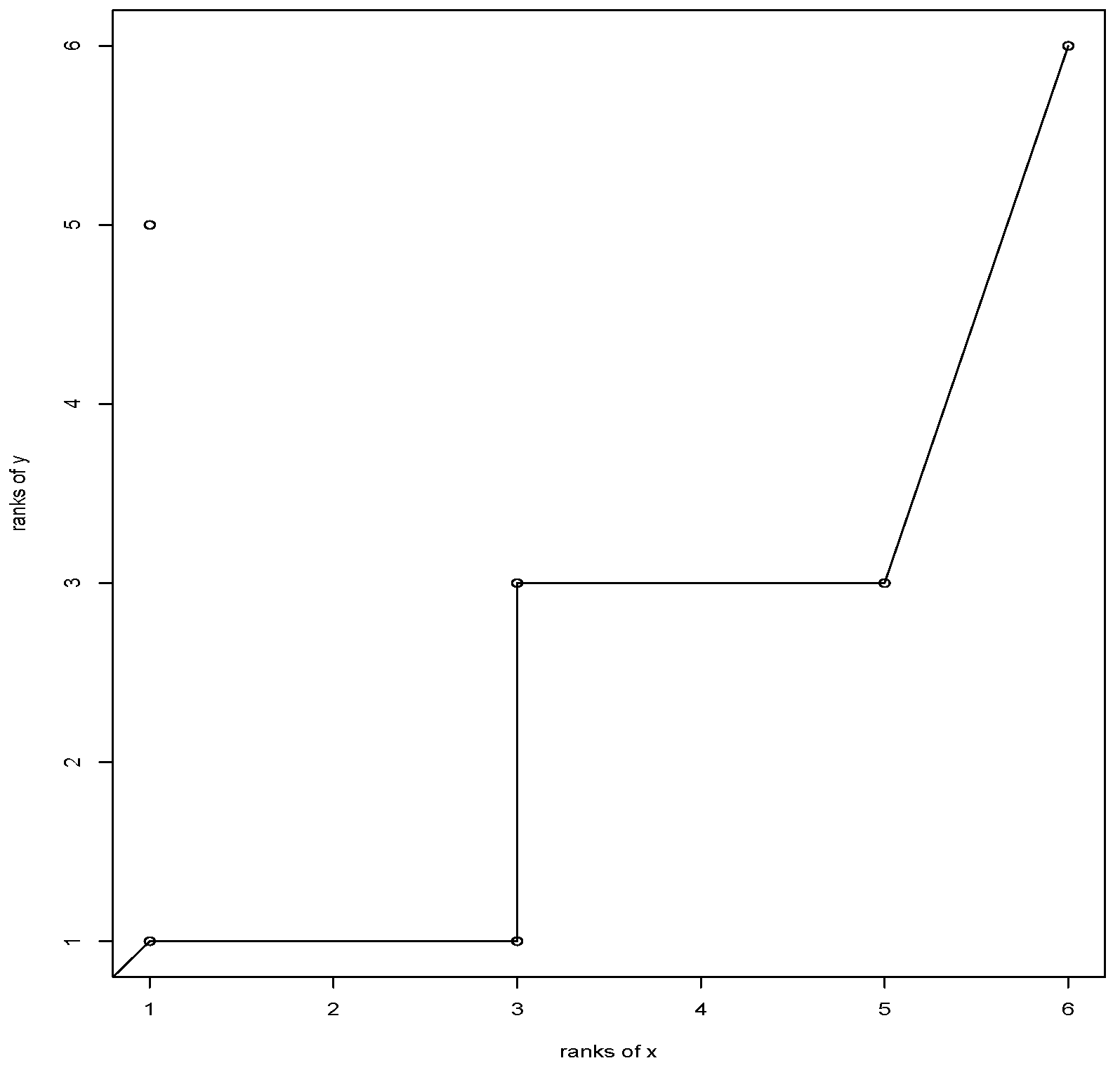
Example 1. Table 1 shows an artificial data with and already ordered in terms of the magnitude of values. We show the graphical construction of This data defines a The maximal non-decreasing subsequence is given by the trajectory from the plot between the ranks of the observations, shown in Figure 1. The value of for this example is 5. We note that the indicated trajectory refers to the correspondence of which is no longer a permutation in the traditional sense since, it allows repetition both in the domain and in the image. Remark 2. Note that the construction of the statistic is symmetric in the sense that if we exchange the roles of X and we obtain the same result. Formally, this characteristic is a consequence of the following property. Consider a sample and the increasing set of indexes such that the trajectory constitutes a non-decreasing subsequence (as illustrated by Example 1), this occurs if and only if and then the trajectory constitutes a non-decreasing subsequence also.
The example shows that the procedure operates in an extended space of the symmetric group
Below we show a motivation to identify the dependence by trajectories such as those used by Definition 2 and exemplified in
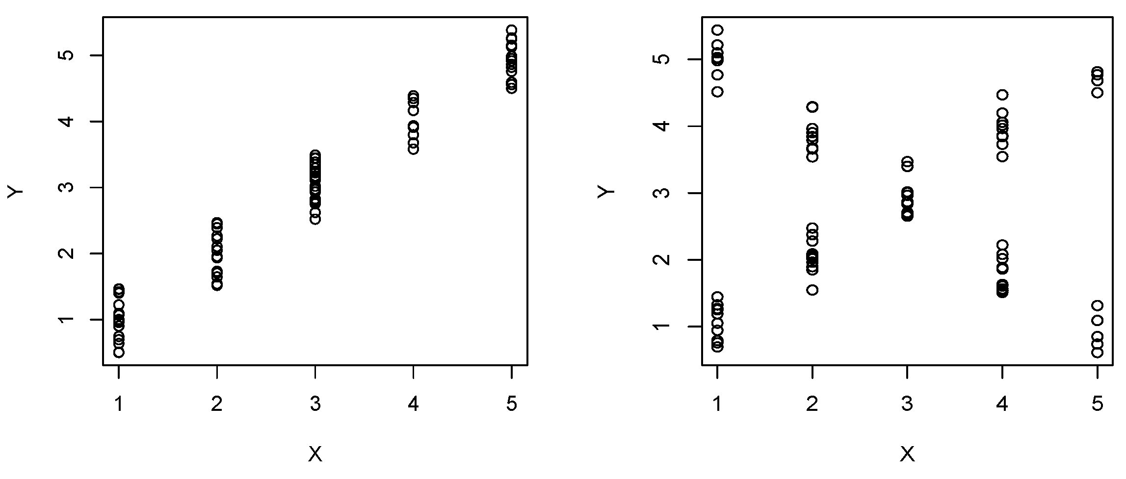
Figure 1. The dependence on a bivariate vector can be represented by the ranks of the observations; let’s see a simple motivation.
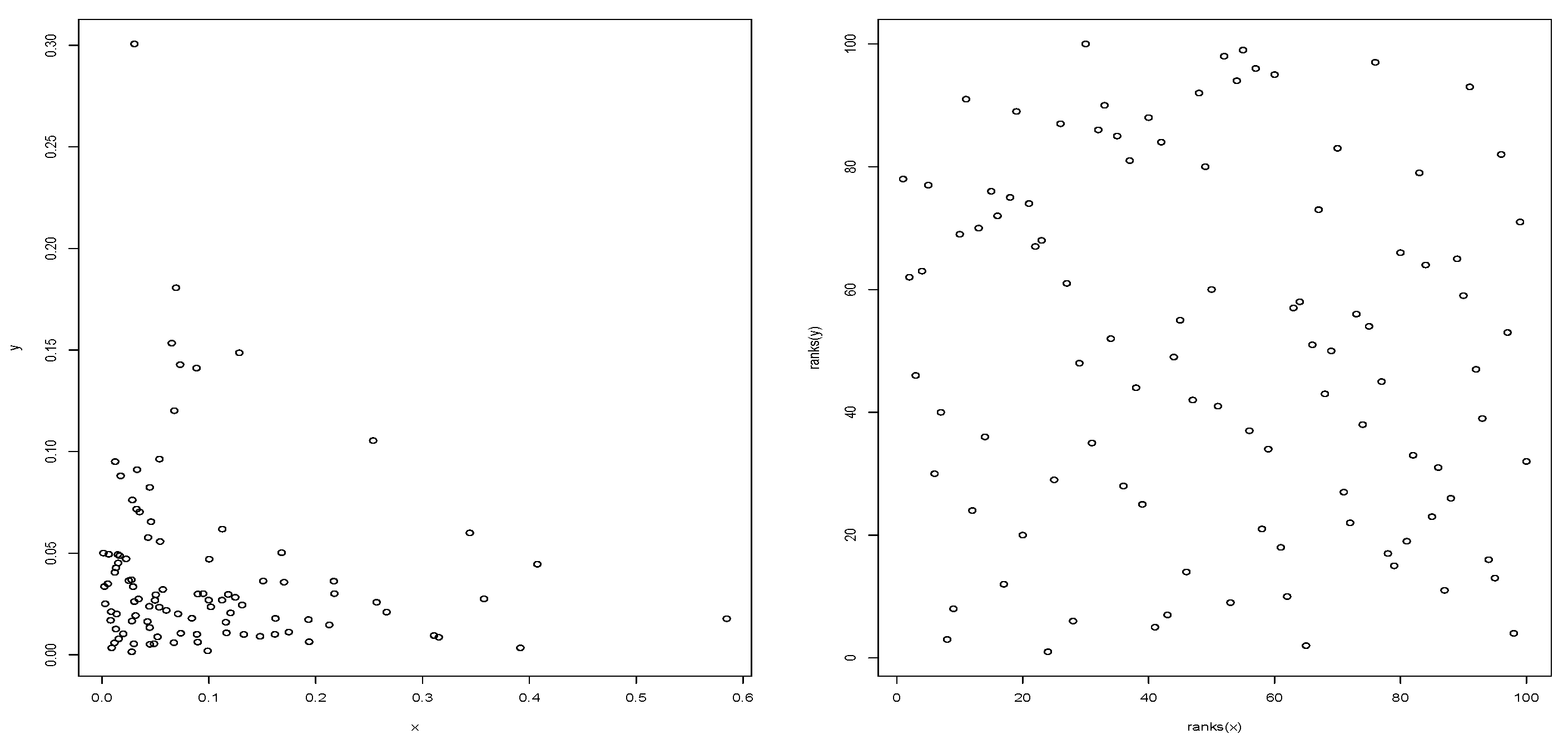
We see on the left of
Figure 2 an apparent relationship between the random variables, this illusion of relationship disappears in the graph on the right, since when computing the ranks of the observations, the marginal stochastic structure is neutralized, showing the dependence between
X and
And, in this case,
X and
Y are independent, since they have been generated in this way. On the other hand, if the variables
X and
Y were dependent,
Figure 2 on the right should expose a pattern, and traces of it would be captured by the
notion.
The formulation of the conjectures of independence between the random variables is then given by
Here follows the test’s statistic build from Definition 2.
Definition 3. Let be replications of . Define where as given by Definition 2, and with .
That is, we consider the notion given by the Definition 2 for each set which include the entire sample except one, allowing to build Then, we define and, the test statistic is the average between all the cases Next we introduce the most frequent formulation of estimation of the two-sided p-value in a context such as that given by the statistic.
Definition 4. The estimator of the two sided p-value for the statistical test of independence between X and Y (see (1)) is defined by,where is the value of calculated in the sample, see Definition 3. is the empirical cumulative distribution function of under independence, and is the indicator function of the set In the following subsection, we analyze the performance of two proposals to estimate
one introduced in [
5] and the other proposed by this paper.
2.1. Estimates
can be estimated by using bootstrap, for instance see [
5]. Denote this kind of estimation as
The procedure to buid
under
hypothesis is replicated here. Let be
B a positive and integer value, we compute
B size
n resamples with replacement of
and
separately, since we assume that
is true. That is, we generate
for
resampling from
and, we generate
for
resampling from
Then, for each
b define
and from that sample compute the notion
from Definition 3, say
Then, if
denotes the cardinal of
set
In
Table 2, we show the performance of the
’ s test based on the computation of the
p-value (Definition 4) according to the Bootstrap technique, given by Equation (
2). We generated
n independent pairs of discrete Uniform distributions from 1 to
and we computed in 1000 simulations, the proportion of them showing a
p-value (Definition 4)
indicating the rejection of
Such a proportion is expected to be close to
in order to control type 1 error. As we can see, when increasing the number of categories
the
level is no longer respected, since the registered proportion always exceeds
In order to improve the control of type 1 error, in this paper is proposed an alternative way to estimate
The Bootstrap method described above and used in [
5] can be modified in order to avoid the removal of any of the observations, following the strategy of swapping them. We consider
and
separately, given
for each
consider a permutation
and define
Similarly, consider a permutation
and define
Then, for each
b define
and from that sample compute the notion
from Definition 3, say
Then, set
Bootstrap generates the estimate by Equation (
2), it considers samples with replacement, which tends to increase the number of ties. For example, if the original sample has no ties, the Bootstrap procedure tends to create ties, leading to longer non-decreasing subsequences. The permutation-based procedure that allows the formulation of Equation (
3) lacks such a tendency, and this principle seems to be a more suitable strategy.
In
Table 3, we show the performance of the
’ s test based on the computation of the
p-value (Definition 4) according to Equation (
3). We implement the same settings used in
Table 2, also we include simulations for
The impact of Equation (
3) allows better control of the type 1 error, we see that in most cases the proportion does not exceed
and when it does it remains close to
Returning to the construction of the hypothesis test (Equation (
1)), we note that the hypothesis
is used in the construction of both types of estimates of the cumulative distribution, Equations (
2) and (
3). For both cases, the observed values
are treated separately, as being independent
by one side and
for other side. Then, the distribution of the length of the LNDSS, under
is estimated by both procedures, which allows computing the evidence against
given by the observed value in the originally paired
sample and applying Definition 4. Moreover, the type 1 error control refers to the ability of a procedure to reject
under its validity. In other words, it represents an unwanted situation, which we must control. In the study presented by
Table 2 and
Table 3, based on the two ways of estimating the cumulative distribution of
(under
) by Equations (
2) and (
3) respectively, we see that fixed a level
Equation (
3) offers better performance than Equation (
2) since it maintains type 1 error at pre-established levels. For this reason, the test based on the statistic
with the implementation given by Equation (
3) is more advisable in practice.
The following section describes the behavior of the test in different simulated situations, in order to identify its strengths and weaknesses.
3. Simulations
To investigate the performance of the
-based procedure, we will aim to determine the rejection ability of the procedure in scenarios with dependence. Our research focuses on the procedure that uses the Equation (
3) to compute the
p-value, given the justification of
Section 2.1. We begin our study considering discrete distributions that we describe below and some mixtures or disturbances of them.
We take discrete uniform distributions on different regions, consider and a fixed values such that and set
- i.
Uniform on
- ii.
Uniform on
- iii.
Uniform on
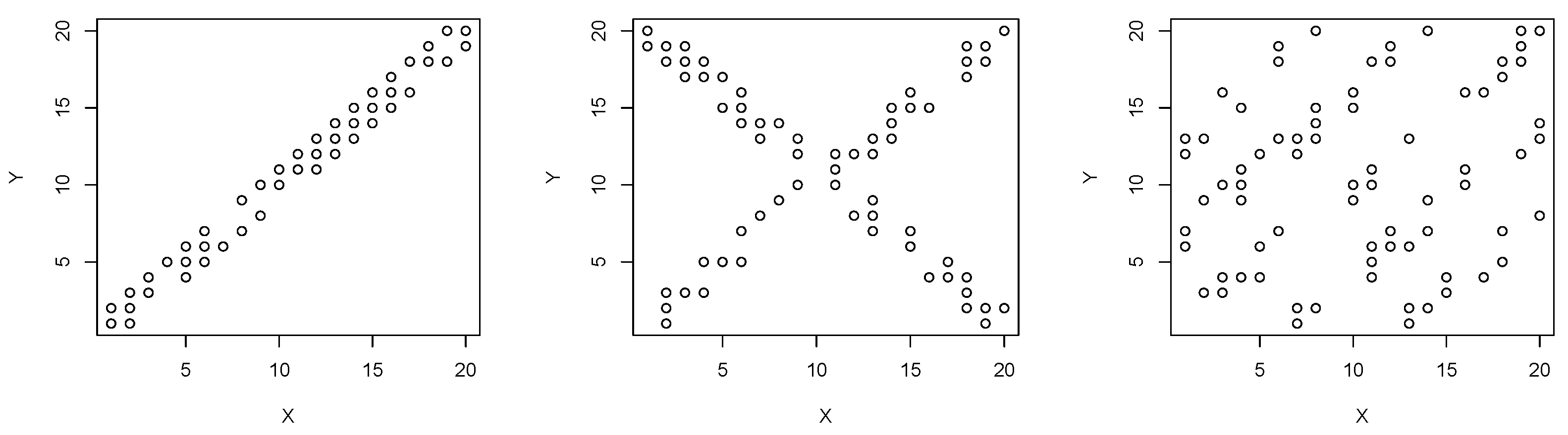
The performance of the distributions i.- iii. is illustrated in
Figure 3, using
and
Denote by
the Uniform distribution on
given
consider now the next three mixture of distributions
- iv.
- v.
- vi.
where the notation
represents that the bivariate vector is given in proportion
p by the distribution
and in proportion
by the distribution
Note that if
we recover the distributions
From
Table 4,
Table 5 and
Table 6, settings have projected that increase the number of categories of the discrete Uniform distribution
and also increase the parameters
a and
Table 4,
Table 5 and
Table 6 show the rejection rates, obtained through 1000 simulations of samples of size
We inspect the distributions
and the mixtures
with
What is sought is to obtain high proportions evidencing the control of type 2 error.
As expected, for distribution the procedure shows maximum performance, for all sample sizes and variants of m and For distribution the performance of the procedure improves and reaches maximum performance as the sample size increases, for all variants of m and For distribution we noticed a deterioration in the performance of the test when compared to the other two cases and despite this, the procedure responds adequately to the sample size, increasing its ability to detect dependence with increasing sample size.
is a distribution that results from disturbing so it makes sense to compare the effect of the disturbance, which in the illustrated cases is 20% from For the distribution the -based procedure shows optimal performance, as occurs in the case In cases and there is a deterioration in the performance of the procedure when compared to and respectively. Despite this, within the framework given by we see that the good properties of the procedure are preserved when the sample size is increased.
In the following simulations, we investigate the dependence between discrete and continuous variables. The types explored are denoted by
and
Figure 4 illustrates the cases. Consider
and set
- vii.
: Uniform distribution on
- viii.
: Uniform on
Denote by the Uniform distribution on given consider now the next two mixture of distributions
- ix.
- x.
Note that when using in ix (or x) we recorver (or ).
Table 7 and
Table 8 show the performance of 1000 simulations of size
from
in
Table 7,
in
Table 8. To the left of each Table (with
), are simulated cases similar to the illustrated in
Figure 4,
and
Table 7 shows that in the case of distribution
the procedure is very efficient and, we see that when the distribution is disturbed (by including 20% from
to the right of
Table 7) the procedure maintains its efficiency in detecting dependence. In relation to the distribution
we see from
Table 8 that two effects occur, the one produced by the sample size
n and the one produced by the value of
By increasing
n and
m the procedure gains power quickly. The same effect is observed in the
distribution (
disturbance), with a certain deterioration in the power of the test.
The
statistic is built in the graph of the paired ranks of the observations, and it is given by the size of the LNDSS found in this graph (see
Figure 1). The proposal induces a region where this statistic can found evidence of dependence, in the diagonal of the graph. The simulation study points that the detection power of the procedure occurs in situations with an increasing pattern in the direction in which the
statistic is built. Even more, the concomitant presence of increasing patterns and decreasing patterns does not necessarily nullify the detection capacity of the procedure, since the statistic
is formulated considering the expanded
space provided with the uniform distribution. See
Table 4,
Table 5,
Table 6,
Table 7 and
Table 8 in which we observe that by increasing the sample size, the detection capacity of
is preserved. Also, looking at the right side of the tables already cited, we verify the robustness of the procedure, when inspecting cases with a concentration of points in the diagonals and suffering contamination, if the sample size grows.
In the next section, we apply the test to real data and compare our results with other procedures.
4. Applying the Test in Real Data
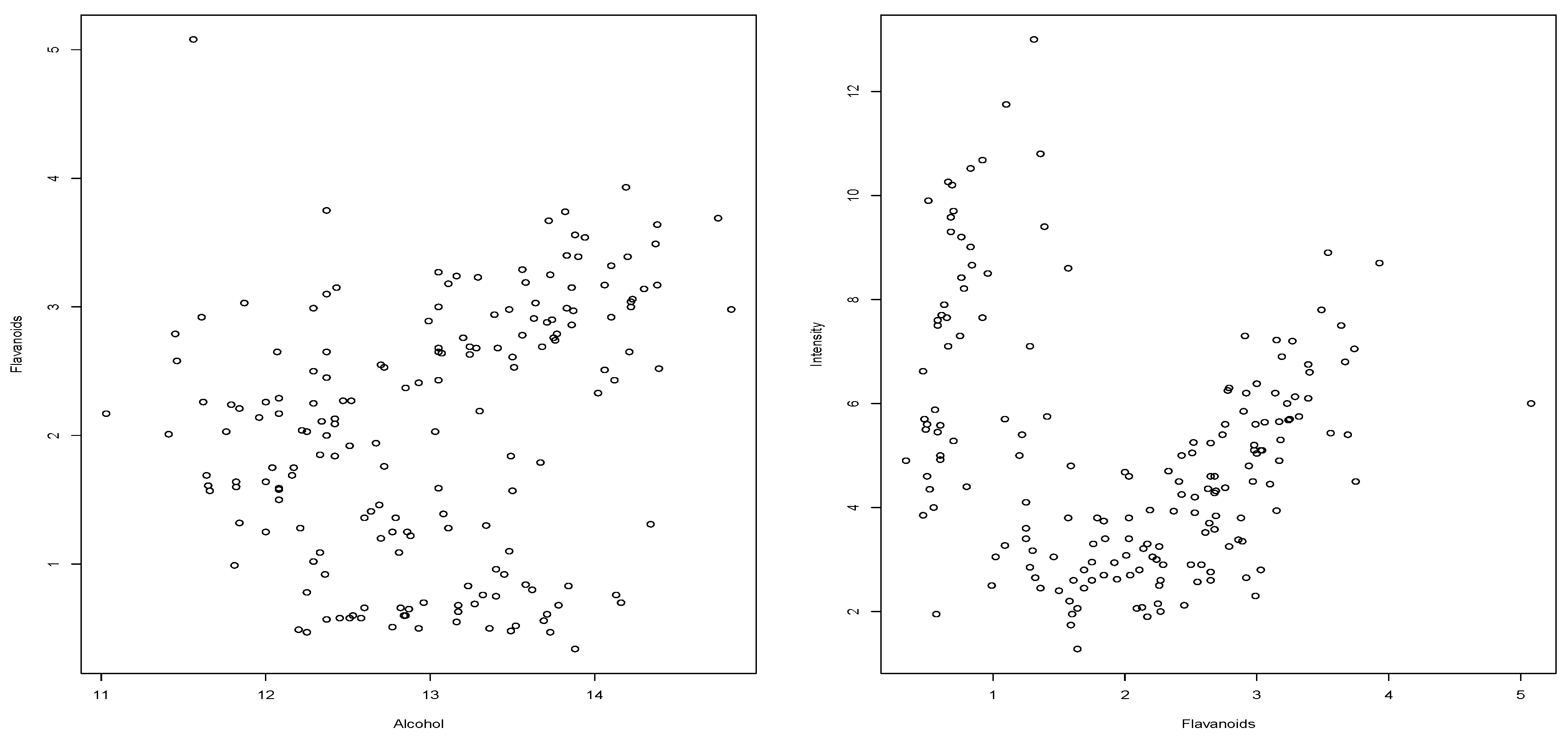
As it has already been commented, in some data sets, we have ties, produced by the precision used in data collection. This is the case of the
wine data set (from the
glus R-package), composed of 178 observations. For example, consider the cases (i)
Alcohol vs.
Flavonoids (see
Figure 5, left) and (ii)
Flavanoids vs.
Intensity (see
Figure 5, right). For each case (i) and (ii) both variables are continuous but recorded with a precision of two decimal places. We use known procedures in the area of continuous variables. For all the computations is used the R-project software environment. The “hoeffd” function in the “Hmisc” package is used to compute the
p-value in the case of Hoeffding’s test. The “cor.test” function in the “stat” package is used to compute the
p-value for Pearson, Spearman and Kendall tests, see also [
8]. Finally, we use the “indepTest” function, from the “copula” package to compute the “Copula“ test.
In case (i) of
Figure 5 (left) all the procedures report
p-value less than 0.02. Using
(
) we obtain
p-value = 0.0160 and
p-value = 0.0004, applying Equations (
2) and (
3), respectively. That is,
-based procedures detect dependence without the possible contraindications that the other procedures have, since we see ties in the dataset.
From the appearance of the scatter plot (
Figure 5, right), it is understandable that the tests based on the Spearman and Kendall coefficients show difficulties in recording dependence, see
Table 9. We also see that the other procedures capture the signs of dependence as well as the one proposed in this paper (
). In both situations (cases (i) and (ii)) the only procedure, without contraindication, with significant
p-value to reject
is
.
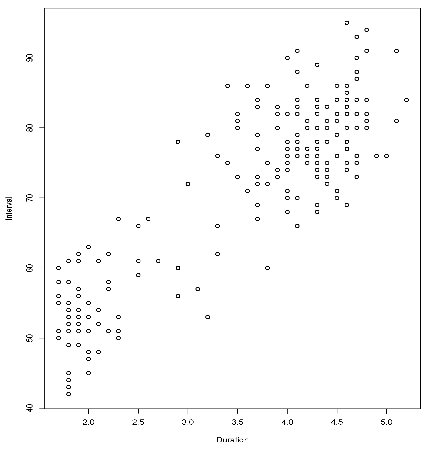
We inspect also the dependence between the variables
Duration: duration of the eruption and
Interval: time until following eruption, both measures in minutes, corresponding to 222 eruptions of the Old Faithful Geyser during August 1978 and August 1979. The data is coming from [
9] and it is a traditional data set used in regression analysis with the aim of predicting the time of the next eruption using the duration of the most recent eruption (see [
10]).
Figure 6 clearly shows the high number of ties, which compromises procedures designed for continuous variables. We have run the
test (
), using various values of
B,
B = 1000, 2000, 5000, 10,000. In all cases the
p-value is less than 0.00001 and using both versions to estimate the cumulative distribution, Equations (
2) and (
3). Then the hypothesis of independence between
Duration and
Interval is rejected.
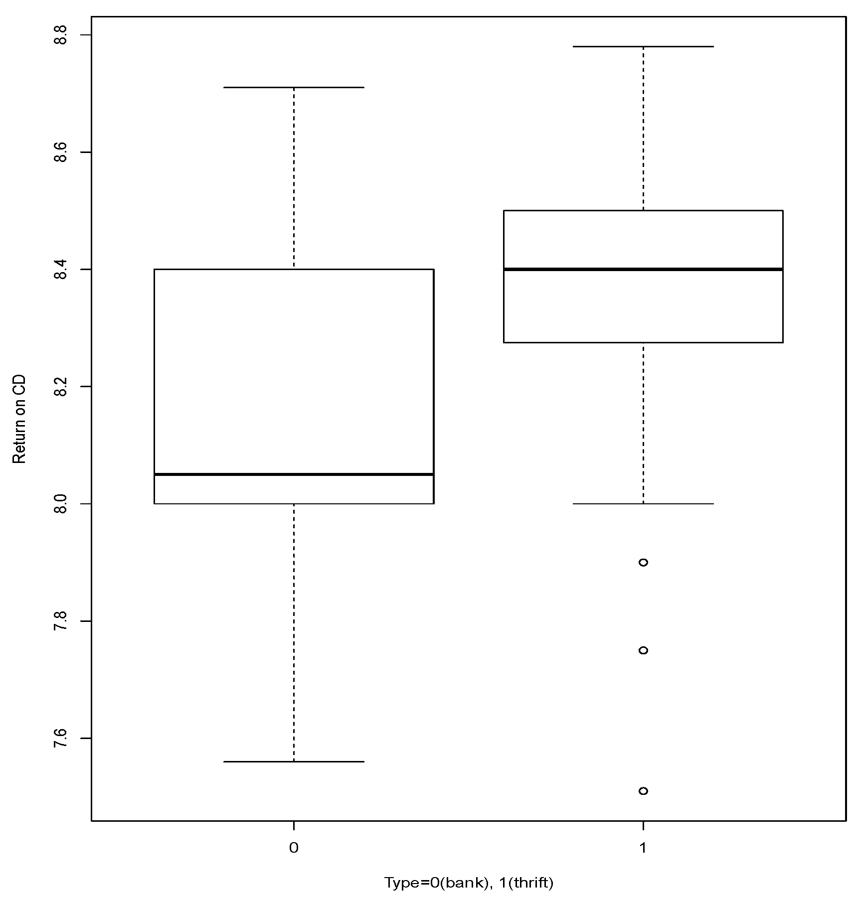
The data set,
cdrate is composed by 69 observations given in the 23 August 1989, issue of
Newsday, it consists of the three-month certificate of deposit rates
Return on CD for 69 Long Island banks and thrifts. The variables are
Return on CD and
Type = 0 (bank), 1 (thrift), source: [
9].
Table 10 shows the data arranged based on the values of the attribute
Return on CD and divided into the two cases of the variable
Type. That table shows sparseness, an issue reported in the literature, that compromises the performance of tests Pearson’s Chi-squared based (
Table 11), see [
1].
In
Table 11 we see the results for testing
We see that according to
’s test we must reject
which seems to be confirmed by
Figure 7.
Figure 7 comparatively shows the performance of variable
Return on CD, for the two values of variable
Type.
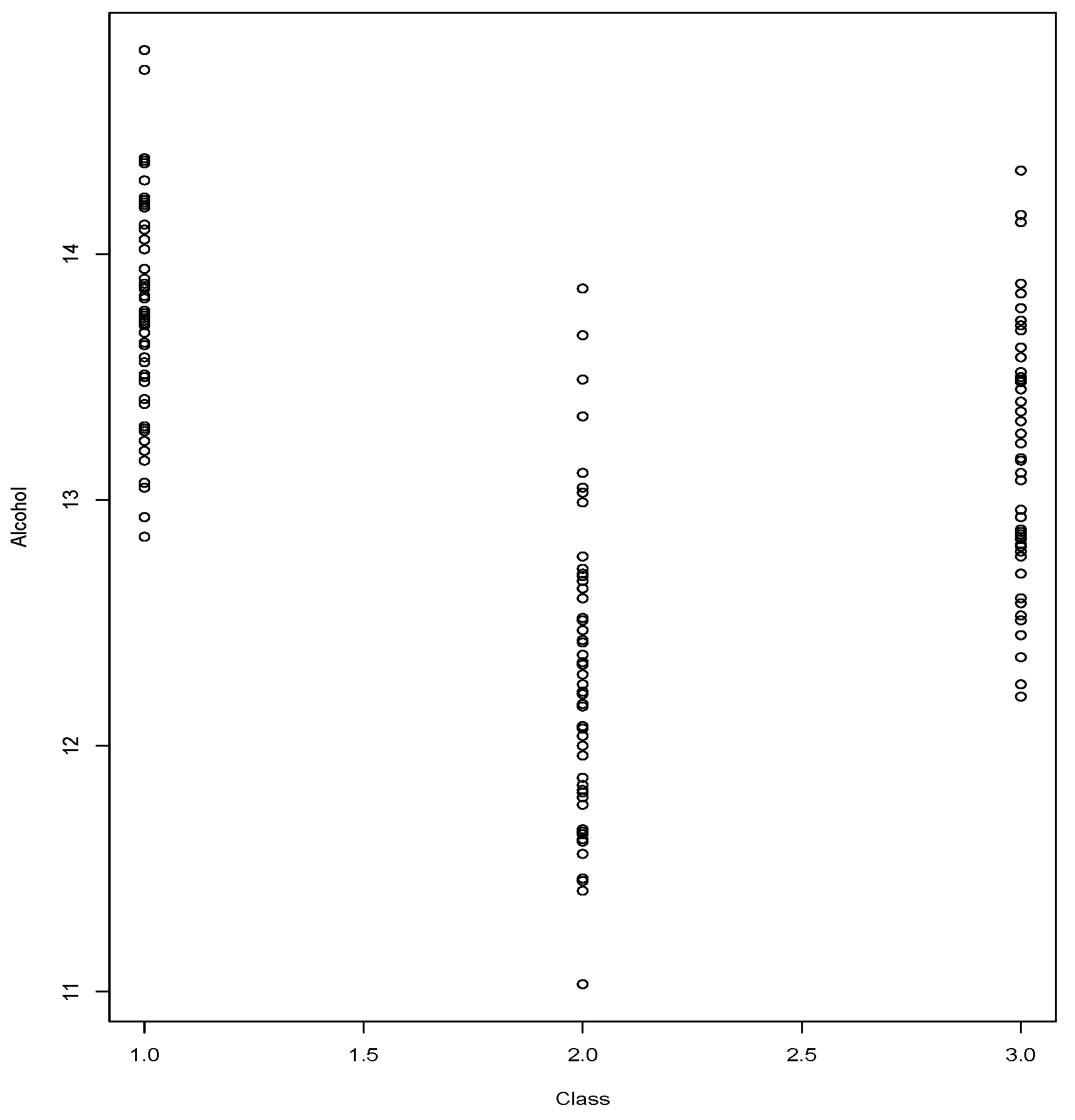
We conclude this section with a case of the
wine data set,
Class vs.
Alcohol.
Figure 8 shows the relationship in which we wish to verify whether independence can be rejected.
Class registers 3 possible values and
Alcohol has been registered with low precision, which leads to observing ties. The observed value of
is
The
p-value given by the Equations (
2) and (
3) indicate the rejection of
By the Equation (
2) we obtain a
p-value = 0.0004 and by the Equation (
3) we obtain a
p-value < 0.00001.
We note that in the cases of
Figure 5 we have verified that the test
through Equation (
3) offers lower
p-value than the version given by Equation (
2). In the cases of
Figure 6 and
Figure 8, it may simply be an effect of computational precision. For the other cases, it is necessary to take into account that the Bootstrap version, by tending to create more ties, shows a tendency to underestimate the cumulative distribution, in other words,
where
is the true cumulative distribution. Due to the increasing tendency shown by the cases addressed (see
Figure 5), it is expected that the observed value of the statistic
in each case is positioned in the upper tail of the distribution, which leads to the
p-value be given by
see Definition 4. As a consequence
With the proposal made through Equation (
3), we seek to correct the underestimation, since it does not favor the proliferation of ties. Which would explain the relationship between the
p-value.


