Enhanced Energy Savings in Indoor Environments with Effective Daylight Utilization and Area Segregation

Abstract

Daylight utilization is one of the key areas for energy savings in indoor environments. An important factor often not considered by the existing daylight utilization approaches is the segregation of the floor into task areas and non-task areas. It is also observed that the inherent asymmetry in the daylight penetration pattern in most indoor environments is not given consideration while designing artificial lighting arrangements. Moreover, daily and annual daylight availability is found to have a symmetrical variation pattern, which is a significant factor often overlooked in utilizing daylight. Thus, the energy assessment can be inaccurate, leading to an incorrect or impractical evaluation of energy savings. This research proposes a comprehensive new approach to assess the energy-saving potential of daylight utilization in indoor environments. This new method combines two approaches to overcome the aforementioned issues. (1) The considered area is segmented into task area and non-task areas (or surrounding area) and considers different levels of required illuminance for each separate area. (2) The variation of available daylight at the considered location is accounted for by dividing the daylight penetration into multiple levels. For the study, the method is first applied to a simulated office space considering real-life parameters, where the annual energy savings were estimated at 83.67%. For further validation, a comparison with a case from an existing method was also carried out, and the proposed method gave an energy saving estimation of 73.45%. This indicates a 10% higher energy saving estimation as compared to the original study, against which the proposed method was compared.

1. Introduction

In the 21st century, sustainability is one of the key factors that is guiding the pathways of economic growth across the globe. Policymakers across the spectrum are giving increased attention to the reduction in energy consumption and the promotion of sustainable technologies to address the growing concerns of diminishing natural resources and rising carbon emissions that are affecting the climate drastically [1]. From residential and commercial energy consumers [2] to large scale industries, energy efficiency is a key design and engineering parameter towards sustainable development [3,4].

For all types of buildings, particularly commercial buildings, lighting represents a significant slice of the energy consumption scenario. In the United States (US), for example, 14% of energy usage in commercial buildings comes from lighting load [5]. The average lighting demand can be even higher, according to some studies [6,7]. Thus, energy-saving measures and techniques in lighting have received the attention of a significant amount of research and development. The reduction in energy consumption in indoor lighting is primarily achieved through two separate yet related avenues. First, considerable research has gone into developing efficient lamps. Studies show that 10–40% of energy savings can be made by the application of lamps with improved efficiency [8]. These upgrades can either require re-designing the existing system design [9] or by much simpler retrofit solutions [10]. Second, a wide range of approaches is employed to reduce electricity consumption by adopting lighting control mechanisms. Studies have shown that the implementation of different lighting control techniques can yield highly beneficial results in terms of annual energy savings [11].

Spaces with proper daylight availability and favorable factors can often achieve the maximum energy savings by implementing daylight-linked lighting controls [12,13]. The factors affecting the actual usable daylight may include orientation and geographic location, dimensions, obstructions, etc.

Methods for the evaluation of energy savings from daylight-linked controls can generally be classified into two groups, which are evaluation through direct measurement and evaluation using estimation methods. The direct measurement methods are studies where the researchers install daylight-linked lighting controls directly in a test room or building and record energy consumption and calculate energy savings [14]. In most cases, the energy consumption is measured for a particular period, such as weeks or months, and the results are then projected for the whole year. Studies that evaluate energy savings through methods which use input parameters from the room and predict energy savings through the application of a methodology is the focus of interest.

Krarti et al. [15] proposed a method that can calculate the percent of energy-saving potential from daylight using room and window parameters. The parameters used are total floor area (A_f), perimeter floor area (A_p), which is a measure of the daylit floor space, and total window glazing area (A_w). Using the building simulation tool DOE-2.1, the researchers modeled these parameters as well as lighting installations. A daylight-linked dimming system was also modeled, which maintained 500 lx illuminance on the workplane. The authors also modeled shading for the windows to prevent excessive heating. The simulation tool gives annual energy saving results in terms of percentage. To establish a relationship between savings percentage and the room parameters, the authors varied the values of two ratios. The ratio A_w/A_p is an indicator of the size of the window to the area of the floor that is lit by daylight, while A_p/A_f indicates the size of the daylit area relative to the total area of the floor. The visible transmittance of the window (${\tau }_w$) also plays a role in daylight penetration. The aforementioned ratios were varied for different values of ${\tau }_w$ and the energy savings were calculated for each case from the DOE-2.1. The resultant curves were used by the researchers to develop a mathematical equation that relates the parameters with the percentage of energy savings$f_d$, as given by Equation (1).

$$f_d=b[1-\exp \left(-a{\tau }_w\frac{A_w}{A_p}\right)]\frac{A_p}{A_f}$$

(1)

The coefficients a and b depend on the building location and control strategy determined by the simulation. The values of these coefficients are determined by Krarti et al. and Ihm et al. [16] for various cities. A detailed description of the methodology can be found in Krarti et al. [15].

To further expand and validate the results of Krarti et al. [15], Ihm et al. [16] studied an office room in Boulder, Colorado, United States of America. The researchers measured the illuminance levels from daylight in the workplane during office hours continuously for four months and then projected those measurements for one whole year using modeling. Based on the method proposed by Ihm et al., a prediction of 63% energy saving was found for the studied office room for the whole year, while the simulated prediction was 64%. Ihm et al. reported very specific details for the room where the method was applied and validated. The researchers reported on the geographic location and orientation of the room, as well as the exact dimension of the room and windows. This provides a good case study as a reference and comparison between an existing method and a newly proposed method in this study.

Li and Tsang [17] used the daylight coefficient (DC) approach in the RADIANCE simulation software. The DC approach was first presented by Tregenza and Waters [18], which takes into account the changes in the illuminance of the sky elements. This method is very effective in predicting indoor daylight illuminance for different locations and sky conditions, and it has been found to give more accurate results than the traditional daylight factor (DF) approach [19,20]. Using the DC approach to determine daylight illuminance is very complex, but modern computer software can make the calculations easier [21]. Several studies have been conducted using the RADIANCE software for the DC approach [20,22,23]. Li and Tsang [17] used RADIANCE to estimate daylight illuminance levels in a daylit corridor using the DC approach. Combining this data with measurements of energy usage of lamps using daylight-linked control systems, a relationship between daylight illuminance levels using the DC approach and the predicted energy savings was developed. It was found that the results showed some variation between the actual energy savings and the savings predicted by the presented model. The results were in agreement for several months, but there were discrepancies for other periods. A similar approach was taken by Kruger and Fonseca [24], where the researchers used a combination of measured and estimated daylight illuminance levels to acquire DC for six classrooms in Curitiba, Brazil.

If we look at some of the more recent approaches for daylight utilization, Sulee et al. [25] experimentally demonstrated a method in which they incorporated a pulse width modulation (PWM) control system directly with the Light Emitting Diode (LED) luminaire, resulting in a reduction in lighting energy consumption. Hajjaj et al. [26], on the other hand, argued that the control system of indoor lighting can be most effective if each individual desk is mapped for lighting level and occupancy status. It must be noted that this ‘distributed intelligent lighting system’, while effective in reducing energy consumption, will also require significant investment for extensive sensor and control system implementation. On a related note, Xiong et al. [27] present that, along with energy saving, visual satisfaction and comfort for the occupants must also be given significant importance, which can be through a ‘personalized’ control approach, making the occupants themselves the decision-makers. A comparison between stepped or proportional dimming control of lighting level with integral reset or switching of luminaires was performed in [28], and it was found that the two approaches can have very similar results in some cases. However, Li et al. found that frequent switching can be detrimental to the life span of the luminaire as well as adverse to occupant satisfaction [29].

As far as the aforementioned methods are concerned, it can be observed that the methods depend on some type of approach that can predict daylight illuminance in the workplane based on room parameters, such as location, dimension of room, windows, and others. These techniques have an established methodology that a researcher or electrical designer can use by taking specific measurements of the room. However, the underlying problem in all of these methods is that these methods are complex methods of calculation. The commonly used methodologies of daylight factor (DF) and daylight coefficients (DC) [18] are very complex [17]. And some methods, like that of Krarti [16], require that the necessary coefficients are already available for a particular location to perform the calculations.

To make it easier to predict daylight illuminance, simulation software packages are used. These software packages can take in the necessary parameters of a room or building and predict daylight illuminance levels in the workplane. These software packages include RADIANCE [20,22,23], DOE-2.1 [16], DLN [24], and others.

By studying the attempts to incorporate daylight utilization with artificial lighting, it can be noted that, on the one hand, the penetration pattern of daylight into any practical indoor environment is asymmetrical. Moreover, the lighting requirements in different areas of the indoor space are also not symmetric. However, on the other hand, the artificial lighting installations are, in most cases, installed in completely symmetrical arrangements. We can also note, as will be illustrated later from simulation results, that the variation of the available daylight illuminance level follows a symmetrical pattern across the span of standard working hours. However, the usage of artificial lighting in indoor scenarios does not take into account this variation, without any proper daylight-linked dimming method. Thus, it is evident that there exist several mismatches between symmetrical and asymmetrical patterns of available daylight and the energy consumption in artificial lighting. Any effective daylight utilization approach should address these inconsistencies to enhance the energy saving potential from daylight utilization.

Although there are some established methods to predict daylight illuminance levels, such as DF and DC, there are no standard procedures that can predict energy savings from the daylight illuminance. The existing methods estimate energy savings that can be achieved by considering practical scenarios and installed control techniques. The inclusion of non-ideal elements, such as window shades to block excessive daylight, minimum dimming value of lamps, modeling of already installed daylight-linked control systems, give a prediction of energy savings that is already achievable in current circumstances. However, the true potential of energy savings should consider more ideal scenarios and estimate the maximum amount of savings achievable. This gives the researchers and engineers the prospect of studying how to gain as much energy savings as possible. The potential of maximum energy savings will provide the researchers and engineers a benchmark to further improve the energy scenarios using advanced technology and better lighting design.

2. Methodology

An early attempt to develop a daylight-linked energy saving estimation method was proposed by the author in [30]. However, that first iteration lacked the modifications required in the methodology to ensure a more valid estimation of energy consumption. In that work, the method was only applied to a test case, simulated at a random geographic location. Moreover, the lighting installations considered in the simulation were not practical as well, considering the type of room simulated. As a result, initial energy consumption calculations, as well as savings estimations, were much higher than practical values. In addition, no comparison with any similar research work was presented, so it was impossible to determine the effectiveness of the method.

The current study takes into account the mentioned shortcomings of the previous work and builds upon it to come up with the proposed version of the methodology.

2.1. Development of the Proposed Method

The study presented in this paper followed the following steps to develop the new approach for daylight utilization:

(1)

Identification of simulation setup: The simulation software is required to model a room and obtain daylight illuminance predictions for the room. There are several criteria that are required from the software that will be used. At first, these requirements were identified. Then, the available software options were explored to find the software that meets the requirements.

(2)

Simulation of a test case and comparative case: Two separate cases were simulated. The first case is the test case, which represents a small private office. The second case is the comparative case. This room was developed based on the case of a previous study, for the purpose of comparison.

(3)

Development of the new method: The exact steps for the calculations in this proposed method were thoroughly developed and articulated. The parameters used for the method and the equations were clearly defined.

(4)

Finally, the calculation steps of the new method were applied to the test case and the comparative case. The calculations were performed using the data obtained from the simulation of the two cases. The final results from the test case gave the potential of annual energy savings from a small, model office room. The comparative case results provided a comparison between the results from a previous method and the new method.

2.2. Identifying the Simulation Platform

The purpose of the simulation was to design a room where the calculation of daylight-linked savings can be performed. There are several software packages that meet the required features for this research. Some of them are DIALux, RADIANCE, DOE-2.1, and DAYSIM. Out of these, DIALux is a software that is easy and quick to implement as it is easy to design the room and its conditions using a comparatively simple user interface, while the others have a steeper learning curve, and some require prior knowledge of programming language to set up the simulations. Due to the simplicity of the room design mechanism in DIALux, designing complex geometry can be troublesome, but for standard room shapes and furniture, DIALux has been proven to be a good solution [31]. This is why DIALux has been used in several past studies for the estimation of daylight and luminaire illuminance levels in simulated rooms [32,33,34]. Thus, DIALux was chosen as the simulation software for this study.

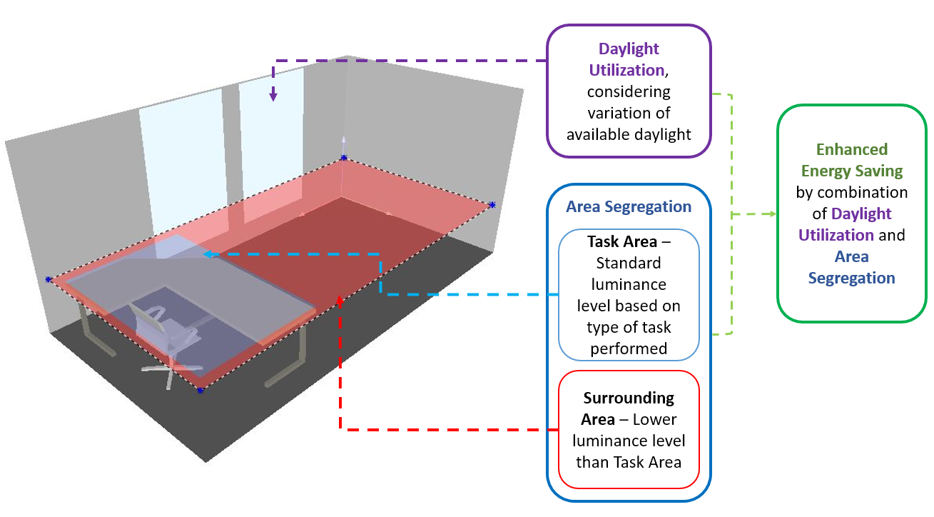
3. Description of the Proposed Method

To address the issues found in similar existing methods, this method highlights two significant factors. First, the separation of areas of the workspace into where critical tasks are performed and spaces for general circulation is undertaken. This is termed as area segregation. Second, the available daylight goes through significant variation, both on a daily and yearly basis. While considering the available natural lighting, this variation must also be given attention. An overview of the method is illustrated in Figure 1.

The proposed method consists of four major steps. For each step, multiple different parameters are required. These parameters are defined with proper symbols assigned to each parameter. Some parameters use values directly acquired from the simulation output while other parameters use equations for the previously introduced parameters. In all cases, the source or the equations used for the values of the parameters are clearly outlined.

3.1. Step 1–General Dimming

The existing lighting scenario of the considered room is the starting point. By comparing the standard required lighting level for the type of room under study and the actual lux levels at the task area and the surrounding areas, the initial level of dimming of the light installations is determined. The new installed load level after this dimming is applied will be taken as the benchmark for the next steps. This increases the accuracy of the estimation of energy savings, omitting savings achievable only by adjustment of installed light fixtures. This issue is often not considered in some of the previous works, which leads to an overestimation of savings [14].

A key issue highlighted in this paper is the separation of the task area and the surrounding area. This separation is considered from this first step. At first, the installed lighting load is separated into two different loads, which are the Initial Task Area Lamps Load (P_TI) and the Initial Surrounding Area Lamps Load (P_SI). For a simple case, these values can be calculated by assigning two groups of the installed luminaire as contributing to the task area and the surrounding area. If the number of luminaires contributing to the task area is N_T and the number of luminaires contributing to the surrounding area is N_S and if the load per installed luminaire is P_L,

$$P_{TI}=P_L\times N_T$$

(2)

and,

$$P_{SI}=P_L\times N_S$$

(3)

The Total Installed Initial Lamps Load is given by

$$P_I=P_{TI}+P_{SI}$$

(4)

The energy-saving potential will depend on the initial illuminance levels from the lamps. Separate values for the task and surrounding areas are calculated. To get these values, the luminaire field is added to the simulated room. The arrangement of the number of rows and the number of luminaires per row should be just that it exceeds the recommended values for the type or room. During this step, the simulation results give the values for Initial Lamps Illuminance Level for the Task Area ($L_{TI}$) and Initial Lamps Illuminance Level for the Surrounding Area ($L_{SI}$).

Based on the type of room under assessment and the lighting level standards to be followed, the Required Illuminance Level for the Task Area ($L_T$) can be determined. For example, the $L_T$ for office rooms, according to the Illuminating Engineering Society of North America (IESNA), is 500 lx. This paper proposes that the illuminance level recommended for the workplane should be associated with the task area of the room, instead of the whole workplane of the room. It is proposed that to enhance energy savings and to identify savings potential, the required level for the surrounding areas of the room (where the critical work is not performed) should be lower than the task area illuminance level. How much lower this illuminance level should be, depends on the preference of the designer or engineer, as there is no standard for surrounding area illuminance levels. This lower illuminance level value is designated as the Required Illuminance Level for Surrounding Area ($L_S$).

Now that the initial and required illuminance levels for the task and surrounding areas are obtained, it is possible to calculate how much dimming can be performed on the initial state to dim the lamps to the required illuminance levels. The amount of reduction in terms of percentage is known as the Power Reduction Factor and is given below:

Power Reduction Factor for Task Area,

$$F_{RT}=1-\frac{L_T}{L_{TI}}(\%)$$

(5)

Power Reduction Factor for Surrounding Area,

$$F_{RS}=1-\frac{L_S}{L_{SI}}(\%)$$

(6)

Now that the dimming amount for the initial lighting scenario is known, the lamps load for the task and surrounding areas after the dimming is applied can be determined. These loads are designated as the Current Lamps Load for task or surrounding areas and can be calculated as:

Current Task Area Lamps Load,

$$P_T=P_{TI}-\left(P_{TI}\times F_{RT}\right)$$

(7)

Current Surrounding Area Lamps Load,

$$P_S=P_{SI}-\left(P_{SI}\times F_{RS}\right)$$

(8)

The Total Installed Lamp Load after general dimming is given by:

$$P_G=P_T+P_S$$

(9)

These load values will be used as the benchmark to compare the final energy savings calculation after daylight dimming.

3.2. Step 2–Frequency Distribution

The different levels of daylight penetration are taken into account at this stage. The illuminance levels in the task and surrounding areas due to the influence of daylight only are necessary for the calculation. For this study, this data is acquired from the DIALux simulation, and this is the main reason for setting up the simulation environment. In collecting data from the simulation, the objective is to get enough data points that can represent the daylight illuminance levels and its variation throughout the year. Data points must be obtained (a) throughout the operating hours of the room and (b) throughout the calendar year. Using the light scenes feature in DIALux, it was possible to get data points for each working hour of the day, and these values were taken for one day of each month. Thus, a total of 132 data values were collected for both task and surrounding areas.

A key highlight of this study was to use three different ranges of daylight penetration levels instead of just one average illuminance level for energy calculations. So the whole range of daylight illuminance levels was divided into three classes or ranges, and the average of each of these ranges would be considered as the illuminance value for that particular range. This division of the set of data points from the illuminance value recordings into multiple ranges can be done using the statistical operation called Frequency Distribution. Three ranges of daylight illuminance levels, i.e., low daylight range, medium daylight range, and high daylight range, would be obtained.

The middle points of each of these ranges would be the three averages used in further steps. For the task area, the three averages are: (a) Task Area Low D/L Average Illuminance Level $(L_{T,LD/L})$, (b) Task Area Medium D/L Average Illuminance Level $(L_{T,MD/L}),$ and (c) Task Area High D/L Average Illuminance Level $(L_{T,HD/L})$. Similarly, for the surrounding area: (a) Surrounding Area Low D/L Average Illuminance Level $(L_{S,LD/L})$, (b) Surrounding Area Medium D/L Average Illuminance Level $(L_{S,MD/L})$, (c) Surrounding Area High D/L Average Illuminance Level $(L_{S,HD/L})$.

In this way, the three different classes or ranges of daylight, and the number of values that are within these ranges are recorded. Thus, the final frequency distribution is completed. This result gives the percentage values of each of the three different ranges, which shows the percentage of the total working hours that get Low, Medium, or High Daylight levels. For the task area, the three values are: (a) Task Area Annual Low D/L Penetration % $\left(F_{LT}\right)$, (b) Task Area Annual Medium D/L Penetration % $\left(F_{MT}\right)$, (c) Task Area Annual High D/L Penetration % $\left(F_{HT}\right)$. Similarly, for the surrounding area: (a) Surrounding Area Annual Low D/L Penetration $\left(F_{LS}\right)$, (b) Surrounding Area Annual Medium D/L Penetration $\left(F_{MS}\right),$ and (c) Surrounding Area Annual High D/L Penetration $\left(F_{HS}\right)$. These percentage values are used to divide the total annual working hours into three different annual working hours that receive Low, Medium, or High daylight levels. This calculation will be performed in Step 4.

These calculations can be performed using any software that can provide statistical calculations. For this paper, Microsoft Excel is used to calculate these values from the daylight illuminance level data acquired from the DIALux simulation.

3.3. Step 3–Daylight Dimming

Now that the three different ranges of daylight for the simulated room, and the average values for the three ranges are obtained, the lighting level from the lamps required for the different ranges can be calculated. The artificial lamps need to be dimmed to such a level that the lamps provide an illuminance level that compensates the available daylight illuminance level and brings the total illuminance level to the standard levels for both the task and surrounding areas. For each of the daylight ranges, the average value of that range combined with the lamp illuminance levels should be equal to the standard illuminance level. Thus, the illuminance levels required from the lamps for the three daylight ranges for both the task and surrounding areas can be calculated. The values for the parameters from the Frequency Distribution are used in this step.

For the task area, the following parameters can be calculated:

Low D/L Lux Level Required at Task Area,

$$L_{T,L}=L_T-L_{T,LD/L}$$

(10)

Medium D/L Lux Level Required at Task Area,

$$L_{T,M}=L_T-L_{T,MD/L}$$

(11)

High D/L Lux Level Required at Task Area,

$$L_{T,H}=L_T-L_{T,HD/L}$$

(12)

Similarly, for the surrounding area:

Low D/L Lux Level Required at Surrounding Area,

$$L_{S,L}=L_S-L_{S,LD/L}$$

(13)

Medium D/L Lux Level Required at Surrounding Area,

$$L_{S,M}=L_S-L_{S,MD/L}$$

(14)

High D/L Lux Level Required at Surrounding Area,

$$L_{S,H}=L_S-L_{S,HD/L}$$

(15)

At this stage, a comparison between the current lamp levels after the general dimming step and the required lamp illuminance levels for the three ranges will be made, and the percentage of reduction in lamp power is the amount of dimming necessary for the lamps will be determined. This is calculated simply as the ratio of the current lamp illuminance levels and the required lamp illuminance levels for a particular range, for both the task and surrounding areas.

For the task area,

Low D/L Power Reduction Factor at Task Area,

$$F_{RT,LD/L}=1-\frac{L_{T,L}}{L_T}(\%)$$

(16)

Medium D/L Power Reduction Factor at Task Area,

$$F_{RT,MD/L}=1-\frac{L_{T,M}}{L_T}(\%)$$

(17)

High D/L Power Reduction Factor at Task Area,

$$F_{RT,HD/L}=1-\frac{L_{T,H}}{L_T}(\%)$$

(18)

Similarly, for the surrounding area,

Low D/L Power Reduction Factor at Surrounding Area,

$$F_{RS,LD/L}=1-\frac{L_{S,L}}{L_S}(\%)$$

(19)

Medium D/L Power Reduction Factor at Surrounding Area,

$$F_{RS,MD/L}=1-\frac{L_{S,M}}{L_S}(\%)$$

(20)

High D/L Power Reduction Factor at Surrounding Area,

$$F_{RS,HD/L}=1-\frac{L_{S,H}}{L_S}(\%)$$

(21)

3.4. Step 4–Energy Calculations

In this step, the first load of the lamps is determined by considering the power reduction factors calculated in the previous step. The current task area and surrounding area lamps’ load were already calculated in the general dimming step. Now, the new load of the lamps for both the task area and the surrounding area after dimming due to daylight availability will be calculated. So the amount of power that can be reduced considering the available daylight will be subtracted from the current lamp loads in all three daylight ranges.

For the task area,

Low D/L Task Area Load,

$$P_{T,LD/L}=P_T-\left(P_T\times F_{RT,LD/L}\right)$$

(22)

Medium D/L Task Area Load,

$$P_{T,MD/L}=P_T-\left(P_T\times F_{RT,MD/L}\right)$$

(23)

High D/L Task Area Load,

$$P_{T,HD/L}=P_T-\left(P_T\times F_{RT,HD/L}\right)$$

(24)

Similarly, for the surrounding area,

Low D/L Surrounding Area Load,

$$P_{S,LD/L}=P_S-\left(P_S\times F_{RS,LD/L}\right)$$

(25)

Medium D/L Surrounding Area Load,

$$P_{S,MD/L}=P_S-\left(P_S\times F_{RS,MD/L}\right)$$

(26)

High D/L Surrounding Area Load,

$$P_{S,HD/L}=P_S-\left(P_S\times F_{RS,HD/L}\right)$$

(27)

To calculate the annual energy consumption, the total annual working hours is required to be known. For Annual Working Days, D and Daily Working Hours, T_D, the Total Working Hours Per Year is simply,

$$T_A=D\times T_D$$

(28)

This total working hours is now divided into three different working hours for which the room gets high, medium, or low daylight levels for both the task and surrounding areas. In other words, the number of hours per year the task and surrounding areas of the room gets high, medium, or low daylight will be determined. This is where the results of annual daylight penetration calculations from Step 2 will be taken into consideration.

For the task area,

Low D/L Working Hours at Task Area,

$$T_{LT}=T_A\times F_{LT}$$

(29)

Medium D/L Working Hours at Task Area,

$$T_{MT}=T_A\times F_{MT}$$

(30)

High D/L Working Hours at Task Area,

$$T_{HT}=T_A\times F_{HT}$$

(31)

Similarly, for the surrounding area,

Low D/L Working Hours at Surrounding Area,

$$T_{LS}=T_A\times F_{LS}$$

(32)

Medium D/L Working Hours at Surrounding Area,

$$T_{MS}=T_A\times F_{MS}$$

(33)

High D/L Working Hours at Surrounding Area,

$$T_{HS}=T_A\times F_{HS}$$

(34)

Considering the initial lamp installations without applying any step of the proposed method, the Total Initial Annual Energy Consumption will be given by

$$E_I=P_I\times T_A$$

(35)

After applying the general dimming step, considering new values for installed lamps load for the task and surrounding areas,

After general dimming, the Total Annual Energy Consumption will be given by:

$$E_G=P_G\times T_A$$

(36)

The energy consumptions after applying the daylight dimming step can now be determined. This energy consumption will be the sum of the energy consumptions at low, medium, and high daylight working hours.

So, after applying daylight dimming,

Total Annual Energy Consumption at Task Area,

$$E_{DT}=\left(P_{T,LD/L}\times T_{LT}\right)+\left(P_{T,MD/L}\times T_{MT}\right)+\left(P_{T,HD/L}\times T_{HT}\right)$$

(37)

and, Total Annual Energy Consumption at Surrounding Area,

$$E_{DS}=\left(P_{S,LD/L}\times T_{LS}\right)+\left(P_{S,MD/L}\times T_{MS}\right)+\left(P_{S,HD/L}\times T_{HS}\right)$$

(38)

Therefore, Total Annual Energy Consumption,

$$E_D=E_{DT}+E_{DS}$$

(39)

As mentioned before, the final savings potential will be measured against the benchmark of the general dimming step. The final result can be calculated as,

Energy Saving Potential from Daylight Utilization,

$$S=\frac{\left(E_G-E_D\right)}{E_G} (\%)$$

(40)

4. Results from the Test Case

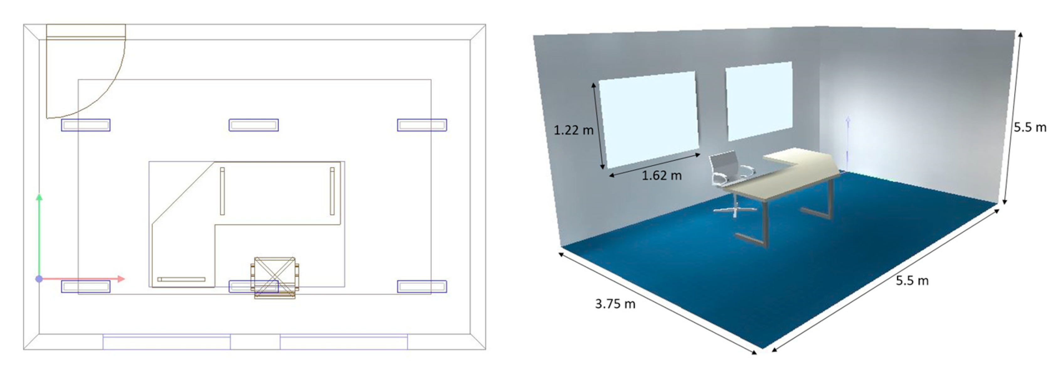
The steps described above for the proposed method was applied to the simulation data for the test case. The CAD view and 3D render of the test case simulation are shown in Figure 2. The room parameters were similar to the previously published work by the authors [30], but the luminaires used in the previous work were not chosen considering practical guidelines. The lamps used in the earlier version delivered far more illuminance levels than lamps that were practically implemented in such an office space simulated in this case. Thus, the energy consumption calculated from the test case results were significantly higher than nominal values. These issues of the previous test case of [30] were resolved in the current test case simulation.

The first step of general dimming shows that the artificial lamps could be dimmed to 10% of full power in the task area and 20% in the surrounding area. This reduction could be achieved just by dimming the lamps down to the required illuminance levels without implementing any automation system. As discussed before, this significant saving is often not considered in savings estimations.

The daylight illuminance levels predicted from DIALux provide several observations. The daylight illuminance data for the test case showed the variation of daylight throughout the working hours. The average illuminance levels for each specific hour throughout the year provided a view of variation in average illuminance from daylight, as shown in Figure 3. It can be seen that the average illuminance level followed a symmetrical pattern across the working hours.

From the graph, it can be seen that the daylight illuminance levels reached a peak at 1 p.m. and the values tapered off towards the end and the start of the working hours. It is also evident from the data set that the difference between the highest and lowest illuminance levels was quite large. The minimum illuminance recorded for the year is just 120 lx for the task area, while the maximum was as high as 895 lx. Similarly, for the surrounding area, the minimum was 71 lx, while the maximum was 532 lx. This variation was taken into consideration in the Frequency Distribution step. The results of this step showed the distribution of illuminance levels for the whole year over three ranges. The distribution in percentage for the task area and the surrounding area are shown in Figure 4.

The figures showed that over 50% of the time during the working hours, both the task and surrounding areas received illuminance levels that fell within the high daylight range, in which maximum savings can be achieved. The daylight dimming calculations showed that the power reduction was 100% for the high daylight range for both the task and surrounding areas, and also for medium daylight range for the task area. This indicates that there was no requirement for artificial lamps during these times, as the required illuminance levels could be fulfilled by daylight alone. It must be noted that this is one of the ideal factors considered in this study to estimate the maximum potential for energy savings. This type of full utilization of daylight is not usually practiced due to issues of visual comfort and heating.

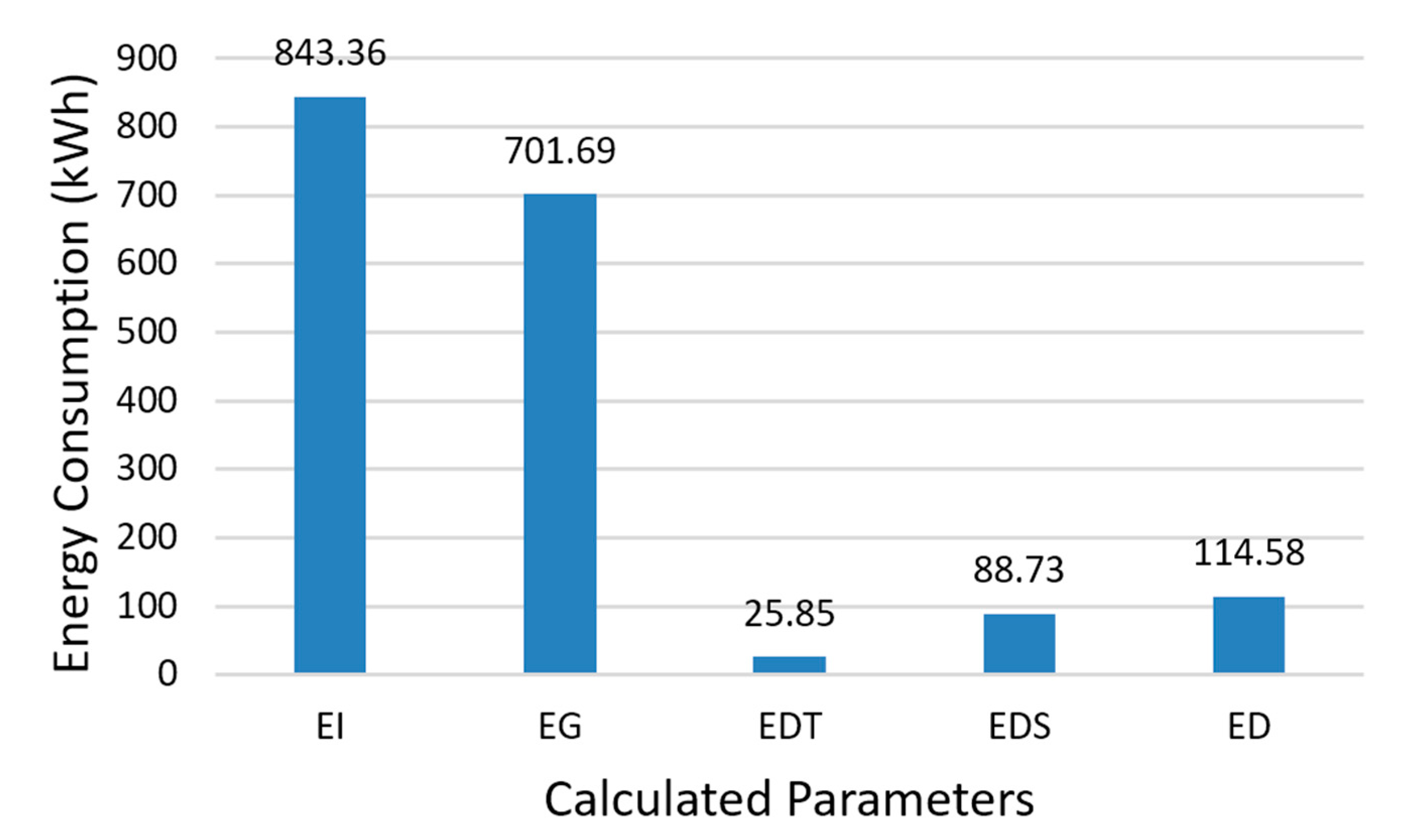
The results from the final step of the energy calculations gave the annual energy consumption and the annual savings potential. The main findings from the energy calculation of the test case are presented in

Table 1. Energy calculation results from the test case.

Calculated Parameter	Result
EI	843.36 kWh
EG	701.69 kWh
EDT	25.85 kWh
EDS	88.73 kWh
ED	114.58 kWh
Energy Saving Potential From Daylight Utilization, S	83.67%

.

Where, E_I is the Total Initial Annual Energy Consumption, E_G represents the Total Annual Energy Consumption after applying general dimming. E_DT gives the Total Annual Energy Consumption at Task Area after daylight dimming, while E_DS is the Total Annual Energy Consumption at Surrounding Area after applying daylight dimming. Then, E_D gives the value of Total Annual Energy Consumption, calculated after applying the previous steps. Finally, the Energy Saving Potential from Daylight Utilization is given by S. All the energy values are given in Kilo Watt Hours (kWh).

After applying Step 1 to Step 4 for the test case, the annual energy consumption was found to be 114.58 kWh. The benchmark for energy savings is the energy consumption after general dimming, which was calculated to be 701.69 kWh. The final annual energy-saving potential of the test case was found to be 83.67%. The results are illustrated graphically in Figure 5.

If the energy savings estimation of the test case is considered, it can be seen that the savings prediction was very high. There are several reasons why the results show such high savings. The entire method was developed in such a way as to give the potential energy saving in an ideal scenario. From the results, daylight ranges were found where the daylight illuminance level was higher than the required illuminance levels. In these cases, the artificial lamps were considered to be dimmed to 0%. In the calculations of this study, the available daylight was considered to be completely usable, whereas, in reality, direct daylight is not always preferred by occupants as the light can be too bright and thus, visually displeasing. Moreover, direct sunlight entrance causes heat build-up in the room, causing discomfort and a higher load on air conditioning. Due to these reasons, window blinds are commonly used to prevent excessive daylight entrance. Thus savings from daylight-linked lighting in practice can be considerably less than that in an ideal scenario.

The room considered in the test case was comparatively small, and the daylight penetration covered almost the entire room. Thus, the effect of daylight was much higher. In a larger room, the further away from the windows, the effect of daylight would be less. Thus, in these cases, the overall illuminance levels from daylight would be less than the smaller room. Another ideal scenario considered was that there was no variation in weather conditions. In real scenarios, the weather pattern can play a significant role in daylight availability. These factors were the significant reasons for the high energy savings potential results obtained for the test case.

5. Comparative Case Results

The steps of the proposed method were also applied to the comparative case simulation, which was based on the study by Ihm et al. [16]. The room used for the comparative case was based on the properties of the room used in the paper by Ihm et al. In this case, the dimension of the room, windows, geographic location, and orientation were all taken into consideration based on the information provided by Ihm et al. The CAD view and 3D render of the comparative case simulation are shown in Figure 6.

The results from the comparative case also showed some interesting observations. The first step of general dimming showed that artificial lamps could be dimmed to 32% of full power in the task area and 44% in the surrounding area. Frequency Distribution of daylight illuminance showed that for both the task and surrounding areas, over a third of the total operating hours fell within the high daylight range, for which there could be 84% dimming in the task area, and 100% dimming in the surrounding area.

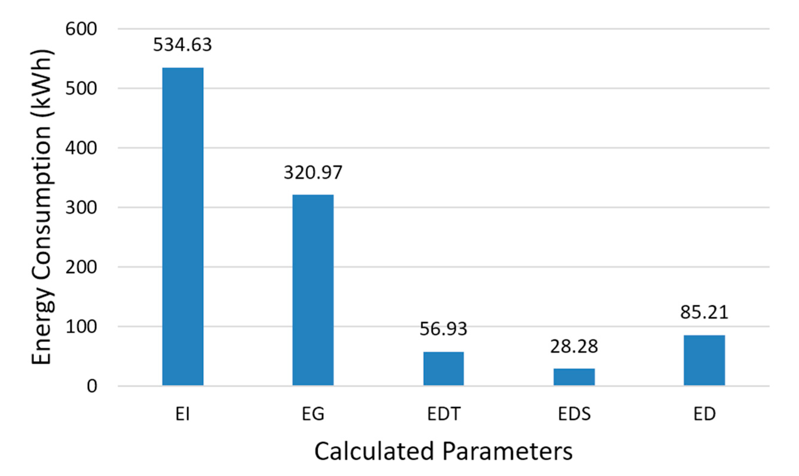
The main findings from this comparative case are shown in

Table 2. Energy calculation results from the comparative case.

Calculated Parameter	Result
EI	534.63 kWh
EG	320.97 kWh
EDT	56.93 kWh
EDS	28.28 kWh
ED	85.21 kWh
Energy Saving Potential From Daylight Utilization, S	73.45%

. The results are graphically illustrated in Figure 7.

Where, E_I is the Total Initial Annual Energy Consumption, E_G represents the Total Annual Energy Consumption after applying general dimming. E_DT gives the Total Annual Energy Consumption at Task Area after daylight dimming, while E_DS is the Total Annual Energy Consumption at Surrounding Area after applying daylight dimming. Then, E_D gives the value of Total Annual Energy Consumption, calculated after applying the previous steps. Finally, the Energy Saving Potential from Daylight Utilization is given by S. All the energy values are given in Kilo Watt Hours (kWh).

As described previously, Ihm et al. suggested that the percentage of the energy-saving estimation can be calculated using Equation (1). The study was validated using the case of an actual office space located in Boulder, Colorado. For this case, the researchers used values for the parameters, as shown in

Table 3. Calculation of savings from Ihm’s method.

Parameter	Value
Total floor area of the building, Af	15.95 m2
Perimeter floor area, Ap	15.95 m2
Perimeter to total floor ratio, Ap/Af	1
Visible transmittance of the window glazing, ${\tau }_w$	0.72
Total window glazing area, Aw	2.32 m2
Daylight aperture, ${\tau }_w\frac{A_w}{A_p}$	0.105
Coefficient a	72.86
Coefficient b	19.36
Percent annual energy savings, fd	63

. The coefficients a and b were estimated using the simulation tool DOE-2.1 for the specific geographic location. The table also shows the energy savings estimation calculated using Equation (1) utilizing these parameters.

To identify the effect of the improvements in the proposed method over the results of Ihm et al., the energy-saving calculations needed to be performed without considering the highlighted factors of the proposed method. The general dimming step was omitted, as this was introduced in the proposed method. Instead of the energy consumption from general dimming (E_G), the initial energy consumption (E_I) was used as the benchmark. In addition, since the separation of the task and surrounding areas was also introduced in the proposed method, this separation was not considered for the purpose of comparison. Hence, the required illuminance levels should be the same for both the task and surrounding areas (500 lx). The illuminance level predictions were considered only for the task area and considered to be the same for the whole workplane. Similarly, the distribution of the daylight levels into three ranges was not considered, and the values for the three ranges were considered to be the same. This means that the low, medium, and high daylight illuminance levels were the same for both the task and surrounding areas, and the value of which will be the average illuminance level of the task area (266 lx). This also means that the distribution of daylight penetration for the three ranges should be all equal, i.e., 33%.

Considering these changes in the values, the energy consumptions and savings estimation were calculated. The results for the comparative case are shown in

Table 4. Results for the comparative case.

Calculation	Benchmark Energy Consumption (kWh)	Energy Consumption After Daylight Dimming (kWh)	Energy Saving (%)
Without considering general dimming, task/surrounding areas, and daylight ranges	481.92	152.79	68.30
Considering all parameters of proposed method	320.97	85.21	73.45

.

The savings predicted by Ihm et al. based on their method was 63%, while the prediction using the proposed method without considering the key parameters was 68.30%. The difference can be due to the use of different software, as each of the lighting simulation software will give slightly different daylight and lamp illuminance predictions. When the complete proposed method (considering all parameters) were applied for the comparative case, the energy consumption after daylight dimming was found to be 85.21 kWh, and the annual savings potential was calculated to be 73.45%. The higher value of savings potential as compared to the results of Ihm et al. is due to the salient features of the method proposed in this study. By taking into account separate illuminance level values and requirements for the task and surrounding areas, and also by considering three ranges of daylight illuminance levels through Frequency Distribution, it is proposed that the overall energy-saving potential of a room can be increased. This point was validated through the increased savings potential resulted from applying the proposed method in the comparative case. Apart from these reasons, the factors mentioned in the discussion of the test case results that could result in higher savings in the test case also apply to the comparative case.

6. Conclusions

A new method for estimating the energy-saving potential from daylight utilization was developed in this study that incorporates steps intended to overcome some prevailing issues with existing methods. Energy saving that could be achieved just by making sure the illuminance level is not significantly above required levels is excluded to make sure the savings estimation reflects the influence of daylight utilization primarily. Further, the workspace was considered to be a combination of task and non-task areas, where the lighting requirements for each were considered differently and met by a blend of artificial and natural lighting. Moreover, the available daylight was categorized into three levels to take into account the variation of natural light availability.

The application of the proposed method using illuminance prediction data resulted in 83.67% saving potential for a simulated private office room used as a test case. Another case study based on a previous research work was carried out for comparison. The results of applying the proposed method without considering the improvement parameters showed 68.30% estimated savings. When the proposed method was applied by considering all the parameters, the results showed 73.45% saving potential, and this energy saving was 10% higher than the original research. Thus, the results obtained validate the effect of the key features of this study. This shows that the new method developed in this study effectively identifies the maximum energy savings potential due to its key features.