Oscillation Properties of Singular Quantum Trees

Abstract

We discuss the possibility of generalizing the Sturm comparison and oscillation theorems to the case of singular quantum trees, that is, to Sturm-Liouville differential expressions with singular coefficients acting on metric trees and subject to some boundary and interface conditions. As there may exist non-trivial solutions of differential equations on metric trees that vanish identically on some edges, the classical Sturm theory cannot hold globally for quantum trees. However, we show that the comparison theorem holds under minimal assumptions and that the oscillation theorem holds generically, that is, for operators with simple spectra. We also introduce a special Prüfer angle, establish some properties of solutions in the non-generic case, and then extend the oscillation results to simple eigenvalues.

1. Introduction

In 1836, Charles Sturm published two seminar papers [1,2] that initiated the comparison and oscillation theory for solutions of second order differential equations and also laid down foundations of the spectral theory of differential operators. Since then, the Sturm comparison and oscillation theory has developed into a broad mathematical field including the study of first order linear differential systems [3], equations with singular coefficients [4,5], partial differential equations on many-dimensional domains [6], higher order equations [7], difference equations [8] and so forth; see the reviews in References [9,10] of the historical developments and the account on important recent progress containing the exhaustive reference lists.

In modern terminology, the classical Sturm oscillation theory considers the Sturm-Liouville eigenvalue problem

$$-\left(p{y}^{\prime }\right){}^{\prime }+qy=\lambda y$$

(1)

on a finite interval $I=[a,b]$, with real-valued functions p and q such that $p>0$ and $1/p$, q are integrable over I, and subject to, for example, the Dirichlet boundary conditions

$$y\left(a\right)=y\left(b\right)=0.$$

(2)

Its results are that, firstly, the eigenvalues ${\lambda }_n$ ($n\in {\mathbb{Z}}_{+}$) of (1)–(2) are real, form an infinite discrete set in $\mathbb{R}$ that is bounded below (and thus accumulates at $+\infty$) and, secondly, that the eigenfunction $y_n$ corresponding to ${\lambda }_n$ has exactly n zeros inside I interlacing those of $y_{n+1}$. The Sturm comparison theorem guarantees that if u and v are solutions of (1) corresponding to $\lambda =\mu$ and $\lambda =\nu$ with $\mu <\nu$, then each nodal domain for u (i.e., each maximal connected component of the set $\{x\in I\mid u(x)\ne 0\}$) contains at least one zero of the solution v.

Over the few last decades, spectral properties of the so-called quantum graphs have been drawing considerable attention. Quantum graphs are differential operators acting on functions defined on metric graphs and satisfying special boundary and interface conditions at their vertices. The interest in quantum graphs stems, in particular, from their wide applicability for modelling nanostructures and networks in for example, nanotechnology, chemistry, superconductivity, optics and so forth; see the review papers in References [11,12] and the books in References [13,14] for particulars of the theory.

One of the first analogues of the oscillation theory for quantum trees was suggested in References [15,16]; it was proved in these papers that generic quantum trees are in many regards similar to the usual Sturm-Liouville operators on an interval; in particular, an eigenfunction corresponding to the nth eigenvalue ${\lambda }_n$ has precisely ${\nu }_n=n$ interior zeros. Vice versa, it was proved in Reference [17] that if the nodal count sequence ${\nu }_n$ of a quantum graph coincides with $\{0,1,2,\dots \}$, then it is a quantum tree.

There are several reasons why the Sturm theory for quantum graphs is much more complicated than for the operators on intervals [18]. One of them is that non-simple eigenvalues are possible, and then different eigenfunctions corresponding to them might have different number of interior zeros; moreover, then there always are eigenfunctions that vanish identically on several edges of the graph, which makes it impossible to count the number of zeros or to discuss zero interlacing properties of solutions. Another complication arises from the cycles; the papers by R. Band, G. Berkolaiko a.o. [19,20,21,22,23] discuss deep dependence between the nodal counts, Betty numbers, and geometric structure of the underlying metric graphs.

The aim of this paper is to answer the question, which of the comparison and oscillation properties continue to hold for the singular quantum graphs, that is, singular Sturm-Liouville operators on metric graphs. Namely, we consider the Sturm-Liouville differential expression

$$-\frac{d^2}{d{x}^2}+q$$

on a metric graph $\mathrm{\Gamma }$, with a potential q belonging to the space $W_2^{-1}\left(\mathrm{\Gamma }\right)$. Generically, such a potential is not a regular function but a distribution; among most typical and most important for applications are the Dirac delta-functions $\delta (·-a)$ and Coulomb-like potentials ${(x-a)}^{-1}$ that are widely used to model interactions between various particles in quantum mechanics.

We shall show that for singular quantum trees the comparison result continues to hold, while the oscillation properties hold generically, that is, for the case where the corresponding operator possesses no non-simple eigenvalues. In addition, we explain that even in the presence of non-simple eigenvalues the oscillation properties remain to hold for simple eigenvalues, by introducing the notion of zero multiplicity of solutions at the tree vertices, thus extending some of the earlier results.

The paper is organized as follows. In Section 2, we collect basic notions and definitions on quantum graphs, and then introduce generalized Prüfer angles in Section 3 and discuss their properties; these are used in Section 4 to derive comparison results on quantum trees. In Section 5 we first prove some spectral properties of singular quantum trees and establish oscillation properties of the generic singular quantum trees. In the Section 6, we introduce the notion of a special solution and a special Prüfer angle, which are then used to derive some spectral properties of non-generic quantum trees. Section 7 contains a summary of the results and several comments on possible extensions, and, finally, some auxiliary results of the Sturm theory for singular Sturm-Liouville operators are collected in Appendix A.

2. Basic Definitions

A quantum graph is a metric graph $\mathrm{\Gamma }$ with differential expression $\tau$ defined on its edges and with interface and boundary conditions prescribed at the vertices. If the graph $\mathrm{\Gamma }$ is connected and contains no loops and cycles, we obtain a quantum tree. Below, we recall the related concepts in more detail.

2.1. Metric Graphs

A geometric graph $\mathrm{\Gamma }=(V,E)$ consists of a set $V=V\left(\mathrm{\Gamma }\right)$ of points (vertices) and a set $E=E\left(\mathrm{\Gamma }\right)$ of edges connecting some of the vertices. A metric graph is a geometric graph, on each edge $\gamma$ of which a metric is defined. Assume the graph $\mathrm{\Gamma }$ is finite and compact, and denote by N the total number of its edges. We can enumerate the edges as ${\gamma }_1,\dots ,{\gamma }_N$; under a natural parametrization, each ${\gamma }_k$ can be identified with an interval $[x_{2k-1},x_{2k}]$ of the real line. Then a vertex v is identified with a subset of equivalent endpoints from ${\left\{x_k\right\}}_{k=1}^{2N}$, and its valency, or degree $d\left(v\right)$ is the number of edges entering v. We say a vertex $v\in V$ is boundary if $d\left(v\right)=1$ and interior otherwise. In what follows, $\partial \mathrm{\Gamma }$ will stand for the set of all boundary vertices of $\mathrm{\Gamma }$ and $I\left(\mathrm{\Gamma }\right)$ for the set of all its interior vertices; also, we set $\mathrm{int}\left(\mathrm{\Gamma }\right):=\mathrm{\Gamma }\backslash \partial \mathrm{\Gamma }$.

A loop is an edge with the same endpoints. We say vertices $v_{*}$ and $v^{*}$ are connected if there exists a sequence of vertices $v_0,v_1,\dots ,v_n$ such that $v_0=v_{*}$, $v_n=v^{*}$, and every two successive vertices $v_j$ and $v_{j+1}$, $j=0,1,\dots ,n-1$, are connected by an edge. If $v_0=v_n$ and $n>1$, the corresponding edges form a cycle. A graph $\mathrm{\Gamma }$ is connected if every two its vertices are connected.

A metric tree is a connected metric graph without loops and cycles. The boundary $\partial \mathrm{\Gamma }$ of the tree $\mathrm{\Gamma }$ is not empty; we take one vertex of $\partial \mathrm{\Gamma }$ and declare it the root $v_0$ (see Figure 1). Once a vertex $v_0$ has been fixed, the tree gets a natural orientation outwards the root. In particular, every edge $\gamma$ connects its beginning (or starting vertex) $a_{\gamma }\in V$ and its end $b_{\gamma }\in V$. Moreover, by saying that ${\gamma }_k$ is identified with $[x_{2k-1},x_{2k}]$ we mean that $x_{2k-1}$ corresponds to the beginning of ${\gamma }_k$ and $x_{2k}$ to its endpoint.

The orientation on the graph allows us to introduce the notion of vertex and edge level. The root $v_0$ gets level zero. The edge starting with $v_0$ is said to be of the first level, and it connects $v_0$ with the vertex of the first level. Similarly, for each $k=1,2,\dots$, any edge beginning with a vertex of level k is then of level $k+1$, and its endpoint is a vertex of level $k+1$. The height of the tree equals the largest level of its vertices (or edges).

2.2. Differential Operators

Since each edge of the tree $\mathrm{\Gamma }$ can be identified with an interval of $\mathbb{R}$, the notions of differentiability or integrability of a function on $\mathrm{\Gamma }\backslash V\left(\mathrm{\Gamma }\right)$ are defined in a standard manner. In particular, for $s\ge 1$, we set

$$L_s\left(\mathrm{\Gamma }\right):={\oplus }_{\gamma \in E\left(\mathrm{\Gamma }\right)}{L}_s\left(\gamma \right)$$

to be the corresponding Lebesgue space on $\mathrm{\Gamma }$. Every function $f\in L_s\left(\mathrm{\Gamma }\right)$ is uniquely determined by its restrictions $f_{\gamma }$ onto the edges $\gamma \in E\left(\mathrm{\Gamma }\right)$ of the graph $\mathrm{\Gamma }$.

As usual, we denote by $W_2^s\left(\gamma \right)$ the Sobolev space of function of order s; in particular, $W_2^1\left(\gamma \right)$ consists of functions whose distributional derivative belongs to $L_2\left(\gamma \right)$. Functions in $W_2^1\left(\gamma \right)$ are absolutely continuous, and we denote by $\stackrel{\circ }{W}{}_2^1\left(\gamma \right)$ the subspace consisting of those of them that vanish at the endpoints of the edge $\gamma$. Then $W_2^{-1}\left(\gamma \right)$ is the space dual to $\stackrel{\circ }{W}{}_2^1\left(\gamma \right)$; every $f\in W_2^{-1}\left(\gamma \right)$ can be written as $f=g^{\prime }$ for some $g\in L_2\left(\gamma \right)$. Finally, we set

$$W_2^{-1}\left(\mathrm{\Gamma }\right):={\oplus }_{\gamma \in E\left(\mathrm{\Gamma }\right)}{W}_2^{-1}\left(\gamma \right).$$

Assume now that q is a real-valued distribution from $W_2^{-1}\left(\mathrm{\Gamma }\right)$ and introduce in the Hilbert space $L_2\left(\mathrm{\Gamma }\right)$ the differential expression $\tau$,

$$\tau :=-\frac{d^2}{d{x}^2}+q.$$

(3)

The action of $\tau$ should be understood edge-wise, that is,

$${\left(\tau y\right)}_{\gamma }:=-y_{\gamma }^{″}+q_{\gamma }{y}_{\gamma }$$

is the restriction of $\tau y$ onto the edge $\gamma \in \mathrm{\Gamma }$. The derivatives are taken in the distributional sense; equivalently, one can define $\tau$ using the regularization by quasi-derivative technique, see References [24,25]. Namely, we take a real-valued function $u\in L_2\left(\mathrm{\Gamma }\right)$ such that $q=u^{\prime }$ and denote by $y^{\left[1\right]}:=y^{\prime }-uy$ the quasi-derivative of an absolutely continuous function y. Now $\tau$ acts via

$$\tau y=-(y^{\left[1\right]}){}^{\prime }-u{y}^{\left[1\right]}-u^{2}y$$

on its domain

$$\mathrm{dom}\tau :=\{y\in L_2\left(\mathrm{\Gamma }\right)\mid \forall \gamma \in E\left(\mathrm{\Gamma }\right),y_{\gamma },y_{\gamma }^{\left[1\right]}\in AC\left(\gamma \right),{\left(\tau y\right)}_{\gamma }\in L_2\left(\gamma \right)\}.$$

2.3. Boundary and Interface Conditions

We prescribe boundary and interface conditions in such a way that the operator on the tree is self-adjoint and boundary/interface conditions are compatible with the vertex structure.

Assume that $v\in I\left(\mathrm{\Gamma }\right)$ is an interior vertex. We denote by ${\gamma }_{+}$ a unique edge entering v and by $B\left(v\right)$ the (nonempty) set of edges starting from v. Then the interface condition at v is of $\delta$-type and reads as follows:

$$\begin{array}{c}y\mathrm{is}\mathrm{continuous}\mathrm{at}v;\end{array}$$

(4)

$$\begin{array}{c}{(y^{\left[1\right]})}_{{\gamma }_{+}}\left(v\right)-\sum _{e\in B\left(v\right)}{(y^{\left[1\right]})}_e\left(v\right)=\alpha \left(v\right)y\left(v\right),\end{array}$$

(5)

with $y\left(v\right)$ denoting the common value of y at the vertex v. We observe that, without loss of generality, one can assume that $\alpha \left(v\right)=0$ as otherwise this can be achieved by replacing the primitive $u_{\gamma }$ of q over the edge ${\gamma }_{+}$ with $u_{{\gamma }_{+}}+\alpha \left(v\right)$. This procedure should be performed consecutively, choosing an interior vertex of the smallest level at each step.

For $\alpha \left(v\right)=0$ the Equation (5) means conservation of the total flux through v and the conditions (4)–(5) are then singular analogues of the standard Kirchhoff interface conditions. In particular, if v is of degree 2, then $B\left(v\right)$ consists of a single edge ${\gamma }_{-}$ starting from v, and (4)–(5) mean that both y and $y^{\left[1\right]}$ are continuous at v. Then one can remove the vertex v and merge the edges ${\gamma }_{+}$ and ${\gamma }_{-}$ to form a single edge ${\gamma }_{+}\cup \left\{v\right\}\cup {\gamma }_{-}$. Therefore, without loss of generality the tree $\mathrm{\Gamma }$ will be assumed to contain no edges of degree 2.

Definition 1. 

The differential expression ℓ is the restriction of τ onto the set of functions satisfying the interface conditions (4) and (5) at every $v\in I\left(\mathrm{\Gamma }\right)$.

At the nonroot boundary vertices $v\in \partial \mathrm{\Gamma }\backslash \left\{v_0\right\}$, we impose the Robin boundary conditions, namely, with $\gamma$ denoting the edge ending with v we set

$${(y^{\left[1\right]})}_{\gamma }\left(v\right)\sin \alpha \left(v\right)=y_{\gamma }\left(v\right)\cos \alpha \left(v\right),$$

(6)

with $\alpha \left(v\right)\in [0,\pi ]$. The boundary condition at the root vertex $v_0$ is introduced in the same manner.

Remark 1. 

If $\alpha \left(v\right)=0$ or $\alpha \left(v\right)=\pi$, then we get the Dirichlet boundary conditions. Otherwise $\alpha \left(v\right)$ can be made equal to $\frac{\pi }{2}$ by changing the primitive u of q over γ by a suitable constant; then the boundary condition becomes of the Neumann type.

Definition 2. 

We denote by $\mathcal{L}$ the restriction of the differential expression ℓ by the boundary conditions (6).

Observe that $\mathcal{L}$ is self-adjoint in $L_2\left(\mathrm{\Gamma }\right)$, see Section 5.1. We are now in a position to define the quantum tree.

Definition 3. 

The quantum tree is a metric tree Γ with symmetric differential expression τ on its edges acting on the functions in $\mathrm{dom}\tau$ satisfying the interface conditions (4)–(5) at the interior vertices $v\in I\left(\mathrm{\Gamma }\right)$ and boundary conditions (6) at the boundary vertices $v\in \partial \left(\mathrm{\Gamma }\right)$.

In other terms, a quantum tree is a metric tree $\mathrm{\Gamma }$ together with the self-adjoint operator $\mathcal{L}$ acting in $L_2\left(\mathrm{\Gamma }\right)$.

3. The Prüfer Angle for Quantum Trees

Unlike for the Sturm-Liouville problems on the intervals, non-trivial solutions of the Sturm-Liouville equation $\ell y=\lambda y$ on the graph $\mathrm{\Gamma }$ may equal zero identically on several edges.

Example 1. 

Consider the star graph with 3 edges $e_1$, $e_2$, and $e_3$ of length 1 joined at the vertex $v_{*}$, see Figure 2. Take $q\equiv 0$, $\lambda ={\pi }^2$, $\alpha \left(v_{*}\right)=0$, and prescribe the Dirichlet boundary condition at the boundary points. Then for every edge $e_j$ there are non-trivial solutions of the equation $\ell y={\pi }^{2}y$ vanishing identically on $e_j$.

Definition 4. 

A solution y to equation $\ell y=\lambda y$ is called non-degenerate if the set $\mathrm{nul}\left(y\right)$ of its interior zeros is discrete.

Given a non-degenerate real-valued solution y of $\ell y=\lambda y$, we can define the Prüfer angle $\theta$ on the tree $\mathrm{\Gamma }$ edge-wise, see Appendix A. On each edge ${\gamma }_k=(x_{2k-1},x_{2k})$, set

$$y\left(x\right)=r\left(x\right)\sin \theta \left(x\right),y^{\left[1\right]}\left(x\right)=r\left(x\right)\cos \theta \left(x\right),x\in (x_{2k-1},x_{2k}),$$

with real-valued $r\left(x\right)$ and $\theta \left(x\right)$; then

$$\cot \theta \left(x\right)=\frac{y^{\left[1\right]}\left(x\right)}{y\left(x\right)}.$$

(7)

In general, $\theta$ is defined only modulo $\pi$; however, we can fix the continuous branch of $\theta$ by prescribing its value at one point. In what follows, we shall usually fix $\theta$ by the condition that $\theta \left(x_{2k}\right)\in (0,\pi ]$ at the endpoint $x_{2k}$.

In this way we define the Prüfer angle $\theta$ on the whole tree $\mathrm{\Gamma }$; as usual, ${\theta }_{\gamma }$ denotes the restriction of $\theta$ onto the edge $\gamma$. We observe that although the solution y of $\ell y=\lambda y$ is continuous at every interior vertex v due to the condition (4), the Prüfer angle $\theta$ need not be continuous there. The reason is that the limiting values of $y^{\left[1\right]}$ at v along adjacent edges may be different, whence different may be the limiting values of $\cot \theta$ and thus of $\theta$. If $y\left(v\right)\ne 0$, we divide the interface condition (5) by $y\left(v\right)$ and get the following matching condition for the limits of $\theta$ at v along the adjacent edges:

$$\cot {\theta }_{{\gamma }_{+}}\left(v\right)=\sum _{e\in B\left(v\right)}\cot {\theta }_e\left(v\right)$$

(8)

(recall that $\alpha \left(v\right)$ was made zero for all interior vertices). If $y\left(v\right)=0$, then ${\theta }_{{\gamma }_{+}}\left(v\right)=\pi$ and ${\theta }_e\left(v\right)=0\mathrm{mod}\pi$ for every $e\in B\left(v\right)$.

Differentiating both sides of (7), one gets the following Riccati equation for $\cot \theta$

$$\frac{d\cot \theta }{dx}=-{(u+\cot \theta )}^2-\lambda ,$$

or, after multiplying through by ${\sin }^2\theta$,

$${\theta }^{\prime }={(u\sin \theta +\cos \theta )}^2+\lambda {\sin }^2\theta .$$

(9)

Remark 2. 

As explained in Appendix A, θ strictly increases at the interior points of every edge γ where it assumes the values $\pi n$, $n\in \mathbb{Z}$ (i.e., at zeros of y on γ).

The differential equation for r reads

$$r^{\prime }=r\left(\frac{1-\lambda -u^2}{2}\sin 2\theta -u\cos 2\theta \right);$$

it can be solved for r once the Prüfer angle $\theta$ is found from (9).

4. The Sturm Comparison Theorem for Quantum Trees

In this section, we establish an analogue of the Sturm comparison theorem for singular quantum trees. We start with the following auxiliary result, with $\mathrm{\Gamma }$ denoting a metric tree and a self-adjoint operator $\mathcal{L}$ introduced on it as discussed in Section 2.

Lemma 1. 

Assume that $y(·;{\lambda }_1)$ and $y(·;{\lambda }_2)$ are non-degenerate solutions of the equations $\ell y={\lambda }_{j}y$, ${\lambda }_1<{\lambda }_2$, on the tree Γ such that

(i) 

neither $y(·;{\lambda }_1)$ nor $y(·;{\lambda }_2)$ vanishes on $\mathrm{int}\left(\mathrm{\Gamma }\right)$;

(ii) 

for every non-root boundary vertex $v\in \partial \mathrm{\Gamma }$,

$$\underset{x\to v}{lim\; sup}\frac{y^{\left[1\right]}(x;{\lambda }_1)}{y(x;{\lambda }_1)}\le \underset{x\to v}{lim\; sup}\frac{y^{\left[1\right]}(x,{\lambda }_2)}{y(x;{\lambda }_2)}.$$

Then

$$\frac{y^{\left[1\right]}(x;{\lambda }_1)}{y(x;{\lambda }_1)}<\frac{y^{\left[1\right]}(x,{\lambda }_2)}{y(x;{\lambda }_2)}$$

for all $x\in \mathrm{int}\left(\mathrm{\Gamma }\right)\cup \left\{v_0\right\}$. The inequality at the interior vertices should be understood edge-wise and at $v_0$ the inferior limits as $x\to v_0$ should be taken.

Remark 3. 

In view of Lemma 2.1 of Reference [4], the superior limits in ii) exist also as the usual limits if $y(v,{\lambda }_j)\ne 0$; if $y(v,{\lambda }_j)=0$, then the corresponding superior limit is equal to $-\infty$.

Proof. 

We start by introducing on $\mathrm{\Gamma }$ the Prüfer angles $\theta (·;{\lambda }_j)$ generated by the solutions $y(·;{\lambda }_j)$, $j=1,2$, as explained in the previous section. Thus the restriction ${\theta }_{\gamma }(·;{\lambda }_j)$ of $\theta (·;{\lambda }_j)$ onto every edge $\gamma =(a,b)$ is continuous on the closure $\overline{\gamma }=[a,b]$, satisfies the relation

$$\cot {\theta }_{\gamma }(·;{\lambda }_j)=y_{\gamma }^{\left[1\right]}(·;{\lambda }_j)/y_{\gamma }(·;{\lambda }_j),$$

and is fixed by the terminal condition ${\theta }_{\gamma }(b;{\lambda }_j)\in (0,\pi ]$. Observe that the equality ${\theta }_{\gamma }(b;{\lambda }_j)=\pi$ holds if and only if $y_{\gamma }(b;{\lambda }_j)=0$. Also, $\theta (·;{\lambda }_j)$ satisfy the matching condition (5) at every interior vertex of $\mathrm{\Gamma }$.

In terms of the Prüfer angles $\theta (·;{\lambda }_j)$ assumptions (i) and (ii) of the lemma read

(i′)

$\theta (·;{\lambda }_j)$ do not assume values $\pi k$, $k\in \mathbb{Z}$, on $\mathrm{int}\left(\mathrm{\Gamma }\right)$;

(ii′)

$\theta (v;{\lambda }_1)\ge \theta (v;{\lambda }_2)$ for every non-root boundary vertex $v\in \partial \left(\mathrm{\Gamma }\right)$.

The properties of the Prüfer angle established in Appendix A guarantee that ${\theta }_{\gamma }(x;{\lambda }_j)\in (0,\pi )$ for all $x\in \gamma$ close enough to b, even if ${\theta }_{\gamma }(b;{\lambda }_j)=\pi$. Assumption (i′) then implies that the values of $\theta (·;{\lambda }_j)$ remain in the interval $(0,\pi )$ on the whole interior $\mathrm{int}\left(\mathrm{\Gamma }\right)$ of the tree $\mathrm{\Gamma }$. Therefore, the claim of the lemma is that under (i′) and (ii′)

$$0\le \theta (x;{\lambda }_2)<\theta (x;{\lambda }_1)<\pi \mathrm{for}\mathrm{all}x\in \mathrm{int}\left(\mathrm{\Gamma }\right)\cup \left\{v_0\right\},$$

(10)

the inequality at the interior vertices being understood edge-wise. Note also that the equality $\theta (x,{\lambda }_2)=0$ can only hold for $x=v_0$.

We shall prove (10) by induction on the number N of edges in the tree $\mathrm{\Gamma }$.

A tree consisting of one edge is an interval $(v_0,v)$, and the statement then follows from Lemma A1. Assume the claim is already proved for all trees consisting of less than $n\ge 2$ edges, and let $N=n$ for a given $\mathrm{\Gamma }$. Consider an edge of $\mathrm{\Gamma }$ of the largest level and denote by a its beginning. Clearly, a differs from $v_0$, whence there is one edge ${\gamma }_{+}$ entering a and $k:=d\left(a\right)-1\ge 1$ edges ${\gamma }_i=(a,v_i)$, $i=1,\dots ,k$, starting from a. Moreover, all vertices $v_i$ are in the boundary $\partial \mathrm{\Gamma }$.

Now at every vertex $v_i$, $i=1,\dots ,k$, we have the inequality $\theta (v_i;{\lambda }_1)\ge \theta (v_i;{\lambda }_2)$. Applying Lemma A1 to the edge ${\gamma }_i$, we conclude that

$$0<{\theta }_{{\gamma }_i}(x;{\lambda }_2)<{\theta }_{{\gamma }_i}(x;{\lambda }_1)<\pi ,x\in {\gamma }_i\cup \left\{a\right\}.$$

Using the interface condition (8) at the vertex a and the fact that the function cot decreases on $(0,\pi )$, we get the relations

$$\begin{array}{cc}\hfill \cot {\theta }_{{\gamma }_{+}}(a;{\lambda }_1)& =\sum _{i=1}^k\cot {\theta }_{{\gamma }_i}(a;{\lambda }_1)\hfill \\ \hfill & <\sum _{i=1}^k\cot {\theta }_{{\gamma }_i}(a;{\lambda }_2)=\cot {\theta }_{{\gamma }_{+}}(a;{\lambda }_2)\hfill \end{array}$$

resulting in the inequality ${\theta }_{{\gamma }_{+}}(a;{\lambda }_1)>{\theta }_{{\gamma }_{+}}(a;{\lambda }_2)$.

Now we consider the tree ${\mathrm{\Gamma }}_a$ obtained by trimming off the edges ${\gamma }_1,\dots ,{\gamma }_k$, see Figure 3. The point a is a new boundary vertex of ${\mathrm{\Gamma }}_a$, and both (i′) and (ii′) hold for the tree ${\mathrm{\Gamma }}_a$. By the induction assumption, we have that $\theta (x;{\lambda }_1)>\theta (x;{\lambda }_2)$ for all $x\in \mathrm{int}\left({\mathrm{\Gamma }}_a\right)\cup \left\{v_0\right\}$. Since

$$\mathrm{int}\left(\mathrm{\Gamma }\right)=\mathrm{int}\left({\mathrm{\Gamma }}_a\right)\cup \left\{a\right\}\cup {\gamma }_1\cup \dots \cup {\gamma }_k,$$

we arrive at (10), thus finishing the proof. □

A nodal domain of a non-degenerate solution y of the equation $\ell y=\lambda y$ is any maximal connected component of $\mathrm{int}\left(\mathrm{\Gamma }\right)$ where y keeps its sign. In other words, a nodal domain is a maximal connected component of the set $\mathrm{int}\left(\mathrm{\Gamma }\right)\backslash \mathrm{nul}\left(y\right)$, where $\mathrm{nul}\left(y\right)$ is the set of all zeros of y in $\mathrm{int}\left(\mathrm{\Gamma }\right)$. Clearly, the number of nodal domains of a non-degenerate solution y exceeds by at least one the cardinality of the set $\mathrm{nul}\left(y\right)$.

An analogue of the Sturm comparison theorem on the interval for a quantum tree reads as follows.

Theorem 1 

(Sturm comparison theorem for quantum trees). Assume that $y(·;{\lambda }_1)$ and $y(·;{\lambda }_2)$ are non-degenerate solutions of the equations $\ell y={\lambda }_{j}y$ with ${\lambda }_1<{\lambda }_2$ such that

(a) 

at the root vertex $v_0$,

$$\underset{x\to v_0}{lim\; sup}\frac{y^{\left[1\right]}(x;{\lambda }_1)}{y(x;{\lambda }_1)}\ge \underset{x\to v_0}{lim\; sup}\frac{y^{\left[1\right]}(x,{\lambda }_2)}{y(x;{\lambda }_2)};$$

(b) 

for every non-root boundary vertex $v\in \partial \mathrm{\Gamma }$,

$$\underset{x\to v}{lim\; sup}\frac{y^{\left[1\right]}(x;{\lambda }_1)}{y(x;{\lambda }_1)}\le \underset{x\to v}{lim\; sup}\frac{y^{\left[1\right]}(x,{\lambda }_2)}{y(x;{\lambda }_2)}$$

Then every nodal domain of $y(·;{\lambda }_1)$ contains a zero of $y(·;{\lambda }_2)$.

Proof. 

We assume, on the contrary, that there is a nodal domain ${\mathrm{\Gamma }}_0$ for $y(·;{\lambda }_1)$, inside which $y(·;{\lambda }_2)$ does not vanish. The boundary points of ${\mathrm{\Gamma }}_0$ either belong to $\partial \mathrm{\Gamma }$ or are interior points of $\mathrm{\Gamma }$ at which $y(·;{\lambda }_1)$ vanishes. The subgraph ${\mathrm{\Gamma }}_0$ is again a tree whose root vertex $v_0^{\prime }$ is the boundary vertex of ${\mathrm{\Gamma }}_0$ of the lowest level in $\mathrm{\Gamma }$; note that (a) holds for $v_0^{\prime }$ instead of $v_0$ no matter whether or not $v_0^{\prime }=v_0$; indeed, if $v_0^{\prime }$ differs from $v_0$, then it is an interior point of $\mathrm{\Gamma }$ so that $y(v_0^{\prime };{\lambda }_1)=0$ and

$$\underset{x\to v_0^{\prime }}{lim\; sup}\frac{y^{\left[1\right]}(x;{\lambda }_1)}{y(x;{\lambda }_1)}=+\infty .$$

Now we introduce the Prüfer angles $\theta (·;{\lambda }_j)$ for the solutions $y(·;{\lambda }_j)$, $j=1,2$, on the tree ${\mathrm{\Gamma }}_0$ in the standard way, that is, $\theta (·,{\lambda }_j)$ are continuous along every edge $\gamma$ and its closure, assume values from $(0,\pi ]$ at the endpoints of the edges, and satisfy the matching condition (8) at interior vertices. We claim that $\theta (·;{\lambda }_1)$ and $\theta (·;{\lambda }_2)$ satisfy on ${\mathrm{\Gamma }}_0$ assumptions (i′) and (ii′) formulated in the proof of Lemma 1. Indeed, (i′) follows from the assumption that $y(·;{\lambda }_j)$ do not vanish on $\mathrm{int}\left({\mathrm{\Gamma }}_0\right)$. Next, if for $v\in \partial {\mathrm{\Gamma }}_0\backslash \left\{v_0^{\prime }\right\}$ it holds $y(v;{\lambda }_1)=0$, then $\theta (v;{\lambda }_1)=\pi \ge \theta (v;{\lambda }_2)\in (0,\pi ]$ by the construction of the Prüfer angle; otherwise, $v\in \partial {\mathrm{\Gamma }}_0\backslash \left\{v_0^{\prime }\right\}$ must be a boundary point of $\mathrm{\Gamma }$ and $\theta (v;{\lambda }_1)\ge \theta (v;{\lambda }_2)$ by assumption (b) and the fact that $\theta (v;{\lambda }_j)\in (0,\pi ]$. In both cases, (ii′) is satisfied for all non-root boundary points of ${\mathrm{\Gamma }}_0$.

Arguments used in the proof of Lemma 1 now result in (10) for the tree ${\mathrm{\Gamma }}_0$ instead of $\mathrm{\Gamma }$. In particular,

$$0\le \theta (v_0^{\prime };{\lambda }_2)<\theta (v_0^{\prime };{\lambda }_1)<\pi ,$$

so that for the restriction ${\theta }_{\gamma }$ of $\theta$ to the edge $\gamma$ starting from the root $v_0^{\prime }$ of ${\mathrm{\Gamma }}_0$ we have the inequality

$$\underset{x\to v_0^{\prime }}{lim}\cot {\theta }_{\gamma }(x;{\lambda }_1)<\underset{x\to v_0^{\prime }}{lim\; inf}\cot {\theta }_{\gamma }(x;{\lambda }_2).$$

This is inconsistent with property (a) for the vertex $v_0^{\prime }$ that was established at the beginning of this proof. The contradiction derived shows that the assumption that the solution $y(·;{\lambda }_2)$ has no zeros on $\mathrm{int}\left({\mathrm{\Gamma }}_0\right)$ was false and thus completes the proof of the theorem. □

5. Oscillation Theorems for Quantum Trees

5.1. General Spectral Properties of a Quantum Tree

Recall that the differential operator $\mathcal{L}$ on the tree $\mathrm{\Gamma }$ is defined as the restriction of the differential expression $\tau$ of (3) onto the functions in $\mathrm{dom}\tau$ satisfying the interface conditions (4)–(5) and the boundary conditions (6). Also, ℓ is the restriction of $\tau$ onto the functions satisfying the interface conditions (4)–(5) at every interior vertex $v\in I\left(\mathrm{\Gamma }\right)$.

Lemma 2. 

The operator $\mathcal{L}$ is self-adjoint, bounded below, and has discrete spectrum.

Proof. 

First we notice that the interface conditions (4)–(5) and the boundary conditions (6) make the operator $\mathcal{L}$ symmetric, which can be verified directly integrating by parts in the expression ${\int }_{\mathrm{\Gamma }}\ell \left(y\right)\overline{y}dx.$

The minimal symmetric operator ${\mathcal{L}}_{\min }$ associated with (3) is the closure of the restriction of $\mathcal{L}$ onto the set of functions with support in $\mathrm{\Gamma }\backslash V$. Clearly, ${\mathcal{L}}_{\min }$ is the direct sum of the minimal operators associated with the restrictions of ℓ to separate edges; thus the operator ${\mathcal{L}}_{\min }$ has finite deficiency indices and its domain consists of all functions in $\mathrm{dom}\mathcal{L}$ satisfying the conditions $y_{\gamma }\left(v\right)=y_{\gamma }^{\left[1\right]}\left(v\right)=0$ for every vertex v and every edge $\gamma$ adjacent to it.

Among the self-adjoint extensions of ${\mathcal{L}}_{\min }$ is the operator ${\mathcal{L}}_{\mathrm{D}}$ defined by the continuity condition (4) and the Dirichlet condition $y\left(v\right)=0$ at every vertex $v\in V$. The operator ${\mathcal{L}}_{\mathrm{D}}$ is the direct sum of the Dirichlet Sturm-Liouville operators on the separate edges; since these latter operators have discrete spectra and are bounded below, the same is true of ${\mathcal{L}}_{\mathrm{D}}$.

We now observe that the deficiency indices of ${\mathcal{L}}_{\min }$ are $(n,n)$, where $n=\dim (\mathrm{dom}{\mathcal{L}}_{\mathrm{D}}$/ $\mathrm{dom}{\mathcal{L}}_{\min })$ is the dimension of the factor-space $\mathrm{dom}{\mathcal{L}}_{\mathrm{D}}/\mathrm{dom}{\mathcal{L}}_{\min }$. In other words, the domain of ${\mathcal{L}}_{\mathrm{D}}$ is obtained from that of ${\mathcal{L}}_{\min }$ by removing n constraints. At every interior vertex $v\in I\left(\mathrm{\Gamma }\right)$ of valency d, $\mathrm{dom}{\mathcal{L}}_{\min }$ imposes $2d$ restrictions, of which only d remain in $\mathrm{dom}{\mathcal{L}}_{\mathrm{D}}$. Likewise, (4)–(5) give d constraints on the functions along the edges starting from v or entering it, and their quasi-derivatives. Similarly, $\mathrm{dom}{\mathcal{L}}_{\min }$ imposes 2 boundary conditions $y\left(v\right)=y^{\left[1\right]}\left(v\right)=0$ at every boundary point $v\in \partial \mathrm{\Gamma }$; in $\mathrm{dom}{\mathcal{L}}_{\mathrm{D}}$ and $\mathrm{dom}\mathcal{L}$, only the Dirichlet condition $y\left(v\right)=0$ or the boundary condition (6) are prescribed at the point v. Therefore, $\dim \left(\mathrm{dom}\mathcal{L}/\mathrm{dom}{\mathcal{L}}_{\min }\right)=n$, whence $\mathcal{L}$ is self-adjoint.

It now follows from Reference [26] that $\mathcal{L}$ has a discrete spectrum and is bounded below along with ${\mathcal{L}}_{\mathrm{D}}$, thus finishing the proof. □

We list the eigenvalues of $\mathcal{L}$ according to their multiplicities as

$${\lambda }_0\le {\lambda }_1\le {\lambda }_2\le \dots$$

and for $\lambda \in \mathbb{R}$ denote by $n\left(\lambda \right)$ the number of eigenvalues of $\mathcal{L}$ counted with multiplicities that do not exceed $\lambda$. The Courant nodal domain theorem is applicable to the quantum graphs and produces the following result.

Lemma 3. 

Assume that λ is an eigenvalue of $\mathcal{L}$ and y is an eigenfunction corresponding to it. Then the number of nodal domains generated by y does not exceed $n\left(\lambda \right)$. In particular, if $\lambda ={\lambda }_n$ is a simple eigenvalue, then y has at most n isolated zeros in $\mathrm{int}\left(\mathrm{\Gamma }\right)$ dividing Γ into at most $n+1$ nodal domains.

Proof. 

We designate by $\mathfrak{l}$ the quadratic form corresponding to the operator $\mathcal{L}$. It is the closure of the quadratic form

$${\mathfrak{l}}_0\left[y\right]:={(\mathcal{L}y,y)}_{L_2\left(\mathrm{\Gamma }\right)}={\int }_{\mathrm{\Gamma }}\ell \left(y\right)\overline{y}dx$$

defined initially on $\mathrm{dom}\mathcal{L}$. By the results of References [24,25], the domain $\mathrm{dom}\mathfrak{l}$ of $\mathfrak{l}$ consists of functions in $W_2^1\left(\mathrm{\Gamma }\right)$ that are continuous on $\mathrm{int}\left(\mathrm{\Gamma }\right)$ and satisfy the boundary conditions (6) at $v\in \partial \mathrm{\Gamma }$ if and only if $\alpha \left(v\right)=0\mathrm{mod}\pi$—that is, only the Dirichlet boundary conditions survive in $\mathrm{dom}\mathfrak{l}$.

By the Courant–Fischer minimax principle [27], $n\left(\lambda \right)$ equals the maximal dimension of a linear subspace M in $\mathrm{dom}\mathfrak{l}$ such that $\mathfrak{l}\left[f\right]\le {\lambda \parallel f\parallel }^2$ for every $f\in M$.

Now assume the eigenfunction y corresponding to an eigenvalue $\lambda$ of $\mathcal{L}$ generates k nodal domains ${\mathrm{\Gamma }}_1$, …, ${\mathrm{\Gamma }}_k$ on $\mathrm{int}\left(\mathrm{\Gamma }\right)$. We denote by $y_j$ the function coinciding with y on ${\mathrm{\Gamma }}_j$ and equal to zero otherwise, and denote by M the linear span of $y_1,\dots ,y_k$. Then $M\subset \mathrm{dom}\mathfrak{l}$ and, upon integrating by parts in the integral ${\int }_{{\mathrm{\Gamma }}_j}\ell \left(y\right)\overline{y}dx$, we see that $\mathfrak{l}\left[f\right]={\lambda \parallel f\parallel }^2$ for every $f\in M$. It thus follows that $k\le n\left(\lambda \right)$ as required. The rest of the claims are simple corollaries of the above. □

5.2. Sturm Oscillation Theory in the Generic Case

Definition 5. 

We call the quantum tree $(\mathrm{\Gamma },\mathcal{L})$ generic if $\mathcal{L}$ possesses no degenerate eigenfunctions.

Lemma 4. 

The spectrum of a generic quantum tree is simple.

Proof. 

Assume that a generic quantum tree $(\mathrm{\Gamma },\mathcal{L})$ has a non-simple eigenvalue $\lambda$; then there are two eigenfunctions $y_1$ and $y_2$ corresponding to $\lambda$ that are non-degenerate and linearly independent. Since $y_1$ and $y_2$ satisfy the same boundary condition (6) at the root vertex $v_0$, there is a non-trivial linear combination $y=c_1{y}_1+c_2{y}_2$ such that $y\left(v_0\right)=y^{\left[1\right]}\left(v_0\right)=0$. Denote by ${\gamma }_0$ the edge starting from $v_0$; then $y_{{\gamma }_0}\equiv 0$ and thus y is a degenerate eigenfunction for the eigenvalue $\lambda$, contrary to the hypothesis that $(\mathrm{\Gamma },\mathcal{L})$ is generic. Thus no eigenvalue of $\mathcal{L}$ can have multiplicity greater than 1, and the proof is complete. □

Lemma 5. 

Assume the quantum tree $(\mathrm{\Gamma },\mathcal{L})$ is generic. Then none of its eigenfunctions can vanish at interior vertices.

Proof. 

Assume y is an eigenfunction of a generic quantum tree $(\mathrm{\Gamma },\mathcal{L})$ that vanishes at an interior vertex v. We prove that the corresponding eigenvalue $\lambda$ then cannot be simple.

Recall that the valency $d\left(v\right)$ of the vertex v is at least 3; therefore, there is one edge ${\gamma }_0$ entering v and $m:=d\left(v\right)-1\ge 2$ edges ${\gamma }_1,\dots ,{\gamma }_m$ starting from v. We denote by ${\mathrm{\Gamma }}_j$, $j=0,1,\dots ,m$, the maximal connected component of $\mathrm{\Gamma }\backslash \left\{v\right\}$ containing the edge ${\gamma }_j$ and by $y_{{\mathrm{\Gamma }}_j}$ the restriction of y onto the ${\mathrm{\Gamma }}_j$. By assumption, for every $j=0,1,\dots ,m$ the function $y_{{\mathrm{\Gamma }}_j}$ does not degenerate on ${\mathrm{\Gamma }}_j$ and $y_{{\mathrm{\Gamma }}_j}\left(v\right)=0$.

Now for every vector $\mathbf{c}:=(c_0,c_1,\dots ,c_m)\in {\mathbb{C}}^{m+1}$ we denote by $y\left(\mathbf{c}\right)$ the function coinciding with $c_j{y}_{{\mathrm{\Gamma }}_j}$ on ${\mathrm{\Gamma }}_j$. By construction, this function solves the equation $\tau y=\lambda y$ on every edge of $\mathrm{\Gamma }$ and verifies the boundary condition (6) at all boundary vertices and the interface conditions (4)–(5) at all interior vertices different from v. At the vertex v the function $y\left(\mathbf{c}\right)$ satisfies the continuity condition (4), while (5) requires that

$$c_0{y}_{{\gamma }_0}^{\left[1\right]}\left(v\right)=\sum _{j=1}^m{c}_j{y}_{{\gamma }_j}^{\left[1\right]}\left(v\right).$$

Observe that none of $y_{{\gamma }_j}^{\left[1\right]}\left(v\right)$ vanishes, as then y would vanish identically on the corresponding edge ${\gamma }_j$; therefore, there is an m-dimensional subspace of vectors $\mathbf{c}=(c_0,c_1,\dots ,c_m)\in {\mathbb{C}}^{m+1}$ solving the above equation. For every such a vector the corresponding function $y\left(\mathbf{c}\right)$ is an eigenfunction of $\mathcal{L}$ for the eigenvalue $\lambda$. As a result, the latter has multiplicity at least $m\ge 2$, contrary to Lemma 4. This contradiction shows that the assumption that y can vanish at an interior vertex was false, thus finishing the proof. □

The Sturm oscillation theorem for generic quantum trees reads as follows.

Theorem 2 

(Sturm oscillation theorem for generic quantum trees). Assume the quantum tree $(\mathrm{\Gamma },\mathcal{L})$ is generic and denote by $y_n$ the (unique up to a multiplicative constant) eigenfunction corresponding to the eigenvalue ${\lambda }_n$. Then $y_n$ has n interior zeros and every nodal domain of $y_n$ contains exactly one zero of $y_{n+1}$.

Proof. 

The proof of the theorem is by induction.

By Lemma 4, the eigenvalues of $(\mathrm{\Gamma },\mathcal{L})$ are simple, so that ${\lambda }_0<{\lambda }_1$. Next, $y_0$ possesses just one nodal domain by Lemma 3 and thus it has no interior zeros. The Sturm comparison Theorem 1 applied to $y_0$ and $y_1$ (corresponding to solutions $y(·,\lambda )$ with $\lambda ={\lambda }_0$ and $\lambda ={\lambda }_1>{\lambda }_0$) shows that $y_1$ has at least one interior zero, and thus exactly one in view of Lemma 3. This establishes the base of induction.

Assume the statement has already been proved for all n less than l. In particular, $y_l$ possesses at least l interior zeros (at least one in each nodal domain of $y_{l-1}$). By Lemma 3, the number of zeros is precisely l, so that they split $\mathrm{\Gamma }$ into $l+1$ nodal domains. By the Sturm comparison Theorem 1, each nodal domain of $y_l$ contains at least one zero of $y_{l+1}$. Since the total number of interior zeros of $y_{l+1}$ cannot exceed $l+1$ by Lemma 3 (as otherwise $y_{l+1}$ would create at least $l+3$ nodal domains), we conclude that the statement of the theorem holds also for $n=l$. This completes the induction step and the proof of the theorem. □

6. Spectral Properties of Non-Generic Quantum Trees

6.1. The Special Solution and the Special Prüfer Angle

In this section, we consider a general quantum tree (that might not be generic) and look for a non-degenerate solution $z(·,\lambda )$ of the equation $\ell y=\lambda y$, $\lambda \in \mathbb{R}$, satisfying the boundary conditions (6) at all non-root boundary vertices. We shall call such a solution special, and the corresponding Prüfer angle $\varphi (·;\lambda )$ is said to be the special Prüfer angle.

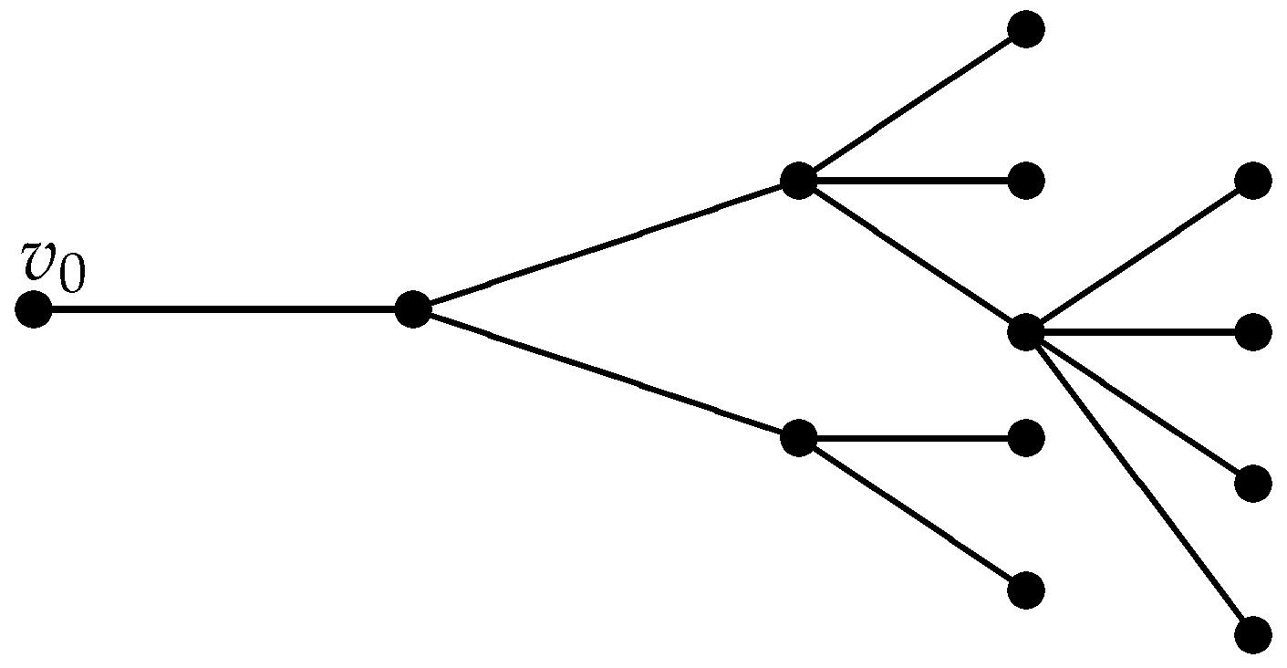
We start with introducing the following notions. For an arbitrary edge $e=(a,b)$ we denote by $\mathrm{\Gamma }\left(e\right)$ the closure of the connected component of the graph $\mathrm{\Gamma }\backslash \left\{a\right\}$ containing the edge e. Thus $\mathrm{\Gamma }\left(e\right)$ is a subtree of $\mathrm{\Gamma }$ with the root vertex a and containing along with e all $x\in \mathrm{\Gamma }$ that can be reached from a moving in positive direction. Further, we denote by $\mathcal{L}\left(e\right)$ the differential operator on the tree $\mathrm{\Gamma }\left(e\right)$ given by the differential expression $\tau$, the interface conditions (4)–(5) for all interior points of $\mathrm{\Gamma }\left(e\right)$, the boundary conditions (6) for all non-root vertices of $\mathrm{\Gamma }\left(e\right)$, and the Dirichlet boundary condition at the root vertex a of $\mathrm{\Gamma }\left(e\right)$. Clearly, $\mathcal{L}\left(e\right)$ is a self-adjoint operator; we denote also by $\mathrm{\Lambda }\left(e\right)$ the spectrum of $\mathcal{L}\left(e\right)$ and set

$$\mathrm{\Lambda }=\bigcup _{e\in E\left(\mathrm{\Gamma }\right)\backslash \left\{e_0\right\}}\mathrm{\Lambda }\left(e\right),$$

where $e_0$ is the edge starting from the root $v_0$. The set $\mathrm{\Lambda }$ is bounded below and discrete.

Lemma 6. 

For every $\lambda \in \mathbb{R}\backslash \mathrm{\Lambda }$, a special solution $z(·;\lambda )$ of the equation $\ell y=\lambda y$ exists, is unique up to a constant factor, and does not vanish at the interior vertices of Γ.

Proof. 

Denote by l the height of the tree $\mathrm{\Gamma }$. We shall prove by the reverse induction in the level k of an edge $e=(a,b)$ that there exists a non-degenerate solution z of $\ell y=\lambda y$ on the subtree $\mathrm{\Gamma }\left(e\right)$ that satisfies the boundary condition (6) at all non-root boundary vertices of $\mathrm{\Gamma }\left(e\right)$. For short, we call such a solution special for $\mathrm{\Gamma }\left(e\right)$. Also, we shall show that a special solution is unique up to a constant factor and vanishes neither at the interior vertices of $\mathrm{\Gamma }\left(e\right)$ nor at the root vertex a of $\mathrm{\Gamma }\left(e\right)$ provided it differs from $v_0$ (i.e., provided $k>1$).

The induction starts from $k=l$ and descends to $k=1$. Assume, therefore, that $e=(a,b)$ is any edge of level l. Then b is a boundary vertex, whence $\mathrm{\Gamma }\left(e\right)=\overline{e}=[a,b]$. We define a special solution z for $\mathrm{\Gamma }\left(e\right)$ as a unique solution of the equation $\tau y=\lambda y$ on $\overline{e}=[a,b]$ subject to the terminal condition

$$y\left(b\right)=\sin \alpha \left(b\right),y^{\left[1\right]}\left(b\right)=\cos \alpha \left(b\right).$$

(11)

We note that z does not vanish at $x=a$; indeed, otherwise $\lambda$ would be an eigenvalue of $\mathcal{L}\left(e\right)$. Clearly, any other solution of $\tau y=\lambda y$ on $\mathrm{\Gamma }\left(e\right)$ satisfying the boundary condition (6) at $x=b$ is a multiple of z so constructed. This gives the base of induction.

Assume that special solutions have already been constructed on the subtrees $\mathrm{\Gamma }\left(e\right)$ for every edge e of level k, $k\le l$, and let $\gamma =(a,b)$ be an edge of level $k-1$. Two possibilities occur depending on whether or not b is a boundary vertex of $\mathrm{\Gamma }$. If $b\in \partial \mathrm{\Gamma }$, then we define the solution z of $\tau y=\lambda y$ on $\mathrm{\Gamma }\left(\gamma \right)=\overline{\gamma }$ as in the previous paragraph, by fixing the terminal conditions (11). If $b\in I\left(\mathrm{\Gamma }\right)$, we denote by ${\gamma }_1,\dots ,{\gamma }_m$ the edges starting from b and by $z_1,\dots ,z_m$ special solutions to $\ell y=\lambda y$ on the subtrees $\mathrm{\Gamma }\left({\gamma }_1\right),\dots ,\mathrm{\Gamma }\left({\gamma }_m\right)$. By the induction assumption, $z_j$ do not vanish at the vertex b; we then consider the solution $y_{\gamma }$ of the equation $\tau y=\lambda y$ on $\overline{\gamma }=[a,b]$ subject to the terminal conditions $y\left(b\right)=1$ and $y^{\left[1\right]}\left(b\right)={\sum }_{j=1}^m{z}_j^{\left[1\right]}\left(b\right)/z_j\left(b\right)$.

Now we construct a function z on the tree $\mathrm{\Gamma }\left(\gamma \right)$ that is equal to $y_{\gamma }$ on the edge $\gamma$ and to $z_j/z_j\left(b\right)$ on each subtree $\mathrm{\Gamma }\left({\gamma }_j\right)$, $j=1,\dots ,m$. Then z is non-degenerate, solves the equation $\tau y=\lambda y$ on each edge constituting the tree $\mathrm{\Gamma }\left(\gamma \right)$ and satisfies the interface conditions (4)–(5) at every interior vertex of $\mathrm{\Gamma }\left(\gamma \right)$ and the boundary conditions at all non-root boundary points of $\mathrm{\Gamma }\left(\gamma \right)$. Therefore, z is the special solution of $\ell y=\lambda y$ on the tree $\mathrm{\Gamma }\left(\gamma \right)$ we wanted to construct. Clearly, such solution is defined up to a multiplicative constant and can be parametrized by its value at b. By construction and the induction assumptions, z does not vanish at interior vertices of $\mathrm{\Gamma }\left(\gamma \right)$. If $a\ne v_0$, then the special solution z does not vanish at the root vertex a as well, as otherwise z would be an eigenfunction of the operator $\mathcal{L}\left(\gamma \right)$ corresponding to the eigenvalue $\lambda$, contrary to the assumption that $\lambda \notin \mathrm{\Lambda }$. This completes the induction step and thus the proof of the lemma.

Corollary 1. 

Assume that $\lambda \in \mathbb{R}\backslash \mathrm{\Lambda }$ and that y is a non-trivial solution of the equation $\ell y=\lambda y$ satisfying the boundary conditions (6) at all non-root boundary vertices. Then y is a multiple of the special solution $z(·,\lambda )$ and thus non-degenerate.

Proof. 

It suffices to show that y cannot vanish at interior vertices of $\mathrm{\Gamma }$: indeed, then y is non-degenerate and thus a multiple of $z(·,\lambda )$ by the above lemma.

Assume, on the contrary, that $y\left(v\right)=0$ for some interior vertex v. We can choose such a v so that y does not vanish identically on all edges adjacent to v as otherwise y would be identical zero on $\mathrm{\Gamma }$. In view of (5), then y is not identical zero on at least two of the adjacent edges. Denote by $e_1,\dots ,e_m$ all the edges starting from v; then the above means that y does not vanish identically on at least one among the subtrees $\mathrm{\Gamma }\left(e_1\right),\dots ,\mathrm{\Gamma }\left(e_m\right)$. However, then $\lambda$ is an eigenvalue for at least one of the operators $\mathcal{L}\left(e_1\right),\dots ,\mathcal{L}\left(e_m\right)$, contrary to the assumption that $\lambda \notin \mathrm{\Lambda }$. The contradiction derived completes the proof. □

Corollary 2. 

Every eigenvalue λ of $\mathcal{L}$ not belonging to Λ is of multiplicity 1 and $z(·;\lambda )$ is the corresponding eigenfunction.

Since the special solution $z(·;\lambda )$, $\lambda \notin \mathrm{\Lambda }$, is unique up to a constant factor, the corresponding special Prüfer angle $\varphi (·;\lambda )$ is unique modulo $\pi$. Clearly, $\varphi (·;\lambda )$ is continuous along each edge but the limiting values at the interior vertices along different adjacent edges need not be the same. Also, the boundary conditions (6) for $z(·;\lambda )$ prescribe the boundary values $\alpha \left(v\right)\in (0,\pi ]$ for $\varphi (·;\lambda )$ at every non-root boundary vertex v. We shall drop the requirement that ${\varphi }_e(b;\lambda )\in (0,\pi ]$ for edges $e=(a,b)$ ending at interior vertices b but gain continuity of $\varphi$ in $\lambda$ instead; note that $\lambda \in \mathrm{\Lambda }$ are not excluded any longer. As usual, for an interior vertex $v\in I\left(\mathrm{\Gamma }\right)$ of valency d the expression $\varphi (v,\lambda )$ should be understood as d limiting values of $\varphi (x,\lambda )$ along every adjacent edge.

Theorem 3. 

For every $\lambda \in \mathbb{R}$, the special Prüfer angle ϕ can be defined so that

(A1) 

for every fixed $x\in \mathrm{int}\left(\mathrm{\Gamma }\right)\cup \left\{v_0\right\}$, $\varphi (x;\lambda )$ is a continuous strictly decreasing function of $\lambda \in \mathbb{R}$;

(A2) 

there is $\mu \in \mathbb{R}$ such that $\varphi (x;\lambda )\in (0,\pi )$ for all $x\in \mathrm{int}\left(\mathrm{\Gamma }\right)\cup \left\{v_0\right\}$ and all $\lambda <\mu$.

For so defined ϕ the following holds:

(A3) 

${lim}_{\lambda \to -\infty }\varphi (x;\lambda )=\pi$ for every fixed $x\in \mathrm{int}\left(\mathrm{\Gamma }\right)\cup \left\{v_0\right\}$;

moreover, if we set

$${\mu }_{*}:=sup\{\mu \in \mathbb{R}\mid \underset{x\in \mathrm{int}\left(\mathrm{\Gamma }\right)\cup \left\{v_0\right\}}{max}\varphi (x;\lambda )>0\mathrm{for}\mathrm{all}\lambda <\mu \},$$

(12)

then

(A4) 

$\varphi (x;{\mu }_{*})>0$ on $\mathrm{int}\left(\mathrm{\Gamma }\right)$ and $\varphi (v_0;{\mu }_{*})=0$.

Proof. 

We shall use the backward induction on the level of the edge $e=(a,b)$ to prove that the special Prüfer angle $\varphi$ can be defined so that it satisfies the stated properties on $\mathrm{\Gamma }\left(e\right)$ instead of $\mathrm{\Gamma }$ and with $v_0$ replaced by the root vertex a of $\mathrm{\Gamma }\left(e\right)$.

An edge $e=(a,b)$ of the maximal level (say l) necessarily ends with a boundary vertex b. Therefore, $\varphi$ on e is defined uniquely as a solution of equation (9) satisfying the initial condition $\varphi \left(b\right)=\alpha \left(b\right)$, and properties (A1)–(A4) for $\varphi$ on $\mathrm{\Gamma }\left(e\right)$ so defined are established in Reference [4], see also Appendix A.

Assume statements (A1)–(A4) have already been proved for the subtrees $\mathrm{\Gamma }\left(e\right)$ with edges e of level k, $k\le l$, and let $\gamma =(a,b)$ be an edge of level $k-1$. Two possibilities occur depending on whether or not b is a boundary vertex of $\mathrm{\Gamma }$. If $b\in \partial \mathrm{\Gamma }$, then $\varphi$ on $\mathrm{\Gamma }\left(\gamma \right)$ is constructed as in the previous paragraph and thus enjoys (A1)–(A4). If $b\in I\left(\mathrm{\Gamma }\right)$, we denote by ${\gamma }_1,\dots ,{\gamma }_m$ the edges starting from b; by induction assumption, on the subtrees $\mathrm{\Gamma }\left({\gamma }_1\right),\dots ,\mathrm{\Gamma }\left({\gamma }_m\right)$ the special Prüfer angle $\varphi$ is well defined and satisfies (A1)–(A4). Set

$$g\left(\lambda \right):=\sum _{j=1}^m\cot {\varphi }_{{\gamma }_j}(b;\lambda );$$

(13)

then g assumes infinite values at the eigenvalues ${\mu }_k$ of $\mathcal{L}\left({\gamma }_1\right)$,..., $\mathcal{L}\left({\gamma }_m\right)$ and by (A1) it is continuous and strictly increasing in between. By virtue of (A2) there is $\mu =\mu \left(\gamma \right)\in \mathbb{R}$ such that $g\left(\lambda \right)$ assumes finite values for $\lambda <\mu$ and, moreover, $g\left(\lambda \right)\to -\infty$ as $\lambda \to -\infty$ in view of (A3).

Set $\beta \left(\lambda \right):=arccotg\left(\lambda \right)\in (0,\pi )$ for $\lambda <\mu$. Then $\beta$ is continuous and strictly decreasing for such $\lambda$. Moreover, the properties of ${\varphi }_{{\gamma }_j}(b;\lambda )$ show that we can extend this definition by continuity to all $\lambda \in \mathbb{R}$, and $\beta \left(\lambda \right)$ will strictly decrease on $\mathbb{R}$. By construction, $\beta \left(\lambda \right)=0\mathrm{mod}\pi$ if and only if ${\varphi }_{{\gamma }_j}(b;\lambda )=0\mathrm{mod}\pi$ for at least one $j\in \{1,\dots ,m\}$.

Now we define ${\varphi }_{\gamma }(·;\lambda )$ on $[a,b]$ as a unique solution of Equation (9) subject to the terminal condition $\varphi (b;\lambda )=\beta \left(\lambda \right)$. Then for $x\in [a,b]$ property (A1) is ensured by Proposition A2, (A3) follows from Lemma A1, and (A2) is established on Step 1 of its proof (see Reference [4]).

Define the number ${\mu }_{*}\left(\gamma \right)$ as in (12) but for the tree $\mathrm{\Gamma }\left(\gamma \right)$ instead of $\mathrm{\Gamma }$; then, clearly,

$${\mu }_{*}:={\mu }_{*}\left(\gamma \right)\le min\{{\mu }_{*}\left({\gamma }_1\right),\dots ,{\mu }_{*}\left({\gamma }_m\right)\}.$$

Assume first that ${\mu }_{*}={\mu }_{*}\left({\gamma }_k\right)$ for some $k\in \{1,\dots ,m\}$. Then ${\varphi }_{{\gamma }_k}(b,{\mu }_{*})=0$ by induction assumption, whence ${\varphi }_{\gamma }(b,{\mu }_{*})=0$ by the definition of $\varphi$. Since the Prüfer angle strictly increases through every point $x_{*}$ were ${\varphi }_{\gamma }(x_{*},{\mu }_{*})=0\mathrm{mod}\pi$, we conclude that ${\varphi }_{\gamma }(x,{\mu }_{*})<0$ for all $x\in [a,b)$, contrary to the definition of ${\mu }_{*}$ and continuity of $\varphi$. Thus ${\mu }_{*}<{\mu }_{*}\left({\gamma }_k\right)$ for every $k=1,\dots ,m$, so that $\varphi (x,{\mu }_{*})>0$ on the set

$$\mathrm{int}\left(\mathrm{\Gamma }\left({\gamma }_1\right)\right)\cup \dots \cup \mathrm{int}\left(\mathrm{\Gamma }\left({\gamma }_m\right)\right)\cup \left\{b\right\}.$$

It remains to prove that ${\varphi }_{\gamma }(x,{\mu }_{*})>0$ for all $x\in (a,b)$ and that $\varphi (a,{\mu }_{*})=0$. Assume, on the contrary, that ${\varphi }_{\gamma }(x_{*},{\mu }_{*})=0$ for some $x_{*}\in (a,b)$. Since ${\varphi }_{\gamma }(·,{\mu }_{*})$ strictly increases through every point where ${\varphi }_{\gamma }(x,{\mu }_{*})=0\mathrm{mod}\pi$, we conclude that ${\varphi }_{\gamma }(x,{\mu }_{*})<0$ for all $x\in [a,x_{*})$. This contradicts continuity of ${\varphi }_{\gamma }$ and the definition of ${\mu }_{*}$ and thus shows that ${\varphi }_{\gamma }(x,{\mu }_{*})>0$ on $\gamma =(a,b)$. Finally, the inequality ${\varphi }_{\gamma }(a,{\mu }_{*})>0$ is ruled out by similar reasons.

The proof of (A4) and of the theorem is complete. □

Remark 4. 

We observe that for $\lambda \notin \mathrm{\Lambda }$ any Prüfer angle $\theta (·;\lambda )$ for the special solution $z(·;\lambda )$ equals the special Prüfer angle $\varphi (·;\lambda )$ modulo π, that is,

$$\cot \theta (·;\lambda )\equiv \cot \varphi (·;\lambda ).$$

(14)

Indeed, both θ and ϕ solve the same differential Equation (9) on every edge e of Γ, satisfy the same boundary conditions $\theta (v;\lambda )=\varphi (v;\lambda )=\alpha \left(v\right)$ for all non-root boundary vertices v, and the same interface conditions at the interior vertices of Γ for $\cot \theta$ and $\cot \varphi$, cf. (8) and the construction of ϕ in the proof of the above theorem.

It turns out that (14) holds even for $\lambda \in \mathrm{\Lambda }$; namely, the following holds true.

Lemma 7. 

Let that $y(·;\lambda )$ be a non-trivial solution of the equation $\ell y=\lambda y$ satisfying (6) for all non-root boundary vertices. Introduce a Prüfer angle θ for the solution y on every edge $\gamma \in E\left(\mathrm{\Gamma }\right)$ where y is non-degenerate; then $\theta (·;\lambda )\equiv \varphi (·;\lambda )\mathrm{mod}\pi$ on all such γ.

Proof. 

On every edge $\gamma =(c,d)$ where y is non-degenerate the Prüfer angles $\theta$ and $\varphi$ solve the same Equation (9) of first order, which is invariant under the shift of $\theta$ or $\varphi$ by $\pi$. Therefore, it suffices to show that the terminal conditions for ${\theta }_{\gamma }$ and ${\varphi }_{\gamma }$ at the vertex d are equal modulo $\pi$. We shall prove the statement for all the subtrees $\mathrm{\Gamma }\left(e\right)$ taken instead of $\mathrm{\Gamma }$ and shall use the backward induction on the level of edge e.

An edge $e=(a,b)$ of the maximal level (say l) necessarily ends with a boundary vertex b. If the solution y is non-degenerate on e, then the Prüfer angle $\theta (·;\lambda )$ satisfies the terminal condition $\varphi (b;\lambda )=\alpha \left(b\right)$ by construction, and the same is true for $\varphi$, resulting in the identity $\theta (·;\lambda )=\varphi (·;\lambda )$ over e.

Assume the lemma has already been proved for the subtrees $\mathrm{\Gamma }\left(e\right)$ with edges e of level k, $k\le l$, and let $\gamma =(a,b)$ be an edge of level $k-1$. The case where $b\in \partial \mathrm{\Gamma }$ is treated as in the previous paragraph. Assume therefore that $b\in I\left(\mathrm{\Gamma }\right)$ and denote by ${\gamma }_1,\dots ,{\gamma }_m$ the edges starting from b. Since

$$\mathrm{\Gamma }\left(\gamma \right)=\gamma \cup \left\{b\right\}{\cup }_{j=1}^m\mathrm{\Gamma }\left({\gamma }_j\right),$$

only the case where y is non-degenerate on $\gamma$ is of interest.

If $y\left(b\right)\ne 0$, then by (8)

$$\cot {\theta }_{\gamma }(b;\lambda )=\sum _{j=1}^m\cot {\theta }_{{\gamma }_j}(b;\lambda ),$$

and by the induction assumption the right-hand side of this relation coincides with

$$\sum _{j=1}^m\cot {\varphi }_{{\gamma }_j}(b;\lambda )$$

giving $\cot {\varphi }_{\gamma }(b;\lambda )$ by the construction of $\varphi$. Thus ${\theta }_{\gamma }(b;\lambda )={\varphi }_{\gamma }(b;\lambda )\mathrm{mod}\pi$, which establishes the induction step.

Now assume that $y\left(b\right)=0$; then ${\varphi }_{\gamma }(b;\lambda )=0\mathrm{mod}\pi$. Observe that y cannot be identical zero on all edges ${\gamma }_1,\dots ,{\gamma }_m$ starting from b as otherwise y must be zero on $\gamma$ as well, and there is nothing to prove. Let therefore y be non-trivial on say the edge ${\gamma }_1$. Then $\theta$ is defined over ${\gamma }_1$ and ${\theta }_{{\gamma }_1}(b;\lambda )=0\mathrm{mod}\pi$, so that ${\varphi }_{{\gamma }_1}(b;\lambda )=0\mathrm{mod}\pi$ by the induction assumption. By the construction of $\varphi$ we get ${\varphi }_{\gamma }(b;\lambda )=0\mathrm{mod}\pi$, thus establishing the induction step and completing the proof. □

Corollary 3. 

$\lambda \in \mathrm{\Lambda }$ if and only if there is an interior vertex v and an edge e starting from it such that ${\varphi }_e(v;\lambda )=0\mathrm{mod}\pi$.

Proof. 

If $\lambda \in \mathbb{R}\backslash \mathrm{\Lambda }$, then by Lemma 6 the special solution $z(·;\lambda )$ exists and does not vanish at any interior vertex $v\in I\left(\mathrm{\Gamma }\right)$. Clearly, this means that the corresponding special Prüfer angle $\varphi (·;\lambda )$ does not assume values $\pi n$, $n\in \mathbb{Z}$, at such vertices.

Let now $\lambda \in \mathrm{\Lambda }\left(e\right)$ for some edge $e=(a,b)$ different from the edge $e_0$ starting from the root $v_0$ of $\mathrm{\Gamma }$. Then there exists an eigenfunction $y(·;\lambda )$, that is, a function that is not identically equal to zero over $\mathrm{\Gamma }\left(e\right)$, solves the equation $\ell y=\lambda y$ on $\mathrm{\Gamma }\left(e\right)$, and satisfies the boundary conditions (6) for all non-root boundary vertices of $\mathrm{\Gamma }\left(e\right)$ and the Dirichlet condition $y(a;\lambda )=0$ at the root vertex a of $\mathrm{\Gamma }\left(e\right)$. We can find an edge $\gamma =(c,d)\in E\left(\mathrm{\Gamma }\right(e\left)\right)$ such that y is non-degenerate on $\gamma$ and $y_{\gamma }(c;\lambda )=0$. Then any Prüfer edge $\theta$ for y on $\gamma$ satisfies ${\theta }_{\gamma }\left(c\right)=0\mathrm{mod}\pi$, and by Lemma 7 we conclude that ${\varphi }_{\gamma }(c;\lambda )=0\mathrm{mod}\pi$ as well. The proof is complete. □

Corollary 4. 

With the number ${\mu }_{*}$ introduced by (12), the following inequalities hold:

$${\lambda }_0\le {\mu }_{*}<min\{\mu \mid \mu \in \mathrm{\Lambda }\};$$

moreover, ${\lambda }_0$ is the only eigenvalue of $\mathcal{L}$ in $(-\infty ;{\mu }_{*}]$.

Proof. 

The second inequality follows from Corollary 3 and (A4). Next, properties (A1), (A3), and (A4) show that there exists a unique ${\lambda }_{*}\le {\mu }_{*}$ such that $\varphi (v_0;{\lambda }_{*})=\alpha \left(v_0\right)$. This means that the special solution $z(·;{\lambda }_{*})$ satisfies the boundary condition

$$\frac{z^{\left[1\right]}(v_0;{\lambda }_{*})}{z(v_0;{\lambda }_{*})}=\cot \varphi (v_0;{\lambda }_{*})=\cot \alpha \left(v_0\right)$$

at the root vertex $v_0$. Therefore, ${\lambda }_{*}$ is an eigenvalue of $\mathcal{L}$ and $z(·;{\lambda }_{*})$ is a corresponding eigenfunction, so that ${\lambda }_0\le {\lambda }_{*}\le {\mu }_{*}$.

We next show that if $\lambda \in (-\infty ;{\mu }_{*}]$ is an eigenvalue of $\mathcal{L}$, then $\lambda ={\lambda }_{*}$. Indeed, as $\lambda \notin \mathrm{\Lambda }$, any corresponding eigenfunction is a multiple of $z(·;\lambda )$ by Corollary 2 and thus is non-degenerate and verifies the boundary condition

$$\frac{z^{\left[1\right]}(v_0;\lambda )}{z(v_0;\lambda )}=\cot \alpha \left(v_0\right)$$

at the root vertex $v_0$. Therefore, $\cot \varphi (v_0;\lambda )=\cot \alpha \left(v_0\right)$; since $\varphi (v_0;·)$ strictly decreases from $\pi$ to 0 as $\lambda$ increases from $-\infty$ to ${\mu }_{*}$, we conclude that $\lambda ={\lambda }_{*}$. This shows that ${\lambda }_{*}$ is the only eigenvalue of $\mathcal{L}$ in $(-\infty ,{\mu }_{*}]$ and thus it is the ground eigenvalue ${\lambda }_0$ of $\mathcal{L}$. □

Corollary 5. 

The ground eigenvalue ${\lambda }_0$ of $\mathcal{L}$ is simple and the corresponding eigenfunction $z(·;{\lambda }_0)$ does not have any zeros in the interior of Γ.

Proof. 

The fact that ${\lambda }_0$ is a simple eigenvalue of $\mathrm{\Gamma }$, with the corresponding eigenfunction $z(·;\lambda )$, follows from the relation $\lambda \notin \mathrm{\Lambda }$ and Corollary 2, while absence of interior zeros of $z(·;\lambda )$ is guaranteed by the inequality ${\lambda }_0\le {\mu }_{*}$ and (A4). □

We stress here the fact that the quantum tree considered here is not assumed generic; thus the simplicity of the ground eigenvalue is not automatic and should have been proved.

Corollary 6. 

A real number $\lambda \notin \mathrm{\Lambda }$ is an eigenvalue of $\mathcal{L}$ if and only if $\varphi (v_0;\lambda )=\alpha \left(v_0\right)\mathrm{mod}\pi$.

Proof. 

According to Corollary 1, for $\lambda \in \mathbb{R}\backslash \mathrm{\Lambda }$ any non-trivial solution y of equation $\ell y=\lambda y$ that satisfies the boundary conditions (6) at all non-root boundary vertices is a multiple of the special solution $z(·,\lambda )$. Therefore, such a $\lambda$ is an eigenvalue of $\mathcal{L}$ and if and only if the special solution $z(·,\lambda )$ satisfies the boundary condition (6) at the root vertex $v_0$ if and only if the special Prüfer angle satisfies the relation $\varphi (v_0;\lambda )=\alpha \left(v_0\right)\mathrm{mod}\pi$. □

6.2. Eigenvalue Multiplicities

The special Prüfer angle can also be used to calculate the multiplicity of non-simple eigenvalues of $\mathcal{L}$; in view of Lemma 4 such eigenvalues necessarily belong to $\mathrm{\Lambda }$ and every corresponding eigenfunction vanishes at some interior vertices.

For every $e=(a,b)\in E\left(\mathrm{\Gamma }\right)$, we denote by $\mathcal{N}(e;\lambda )$ the subspace of $\mathcal{H}\left(e\right):=L_2\left(\mathrm{\Gamma }\left(e\right)\right)$ consisting of all solutions of the equation $\ell y=\lambda y$ on $\mathrm{\Gamma }\left(e\right)$ satisfying the boundary conditions (6) for all non-root boundary vertices v in $\partial \mathrm{\Gamma }\left(e\right)$, and set

$${\mathcal{N}}_0(e;\lambda )=\{y\in \mathcal{N}(e;\lambda )\mid y\left(a\right)=0\}.$$

Further, we denote by $n(e;\lambda )$ and $n_0(e;\lambda )$ the dimensions of $\mathcal{N}(e;\lambda )$ and ${\mathcal{N}}_0(e;\lambda )$ respectively. It follows from Lemma 7 that ${\mathcal{N}}_0(e;\lambda )=\mathcal{N}(e;\lambda )$ if ${\varphi }_e(a;\lambda )=0\mathrm{mod}\pi$. We shall prove that otherwise ${\mathcal{N}}_0(e;\lambda )$ is a proper subspace of $\mathcal{N}(e;\lambda )$ and, moreover, establish the formula for $n(e;\lambda )$ and $n_0(e;\lambda )$.

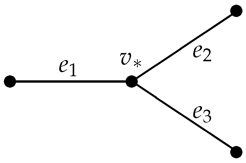
To begin with, we set

$$\chi (e;\lambda )=\left\{\begin{array}{cc}0\hfill & \mathrm{if}{\varphi }_e(a;\lambda )\ne 0\mathrm{mod}\pi ,\hfill \\ 1\hfill & \mathrm{if}{\varphi }_e(a;\lambda )=0\mathrm{mod}\pi .\hfill \end{array}\right.$$

Also, for $v\in I\left(\mathrm{\Gamma }\right)$ that is of valency $m+1\ge 3$ we denote by ${\gamma }_1,\dots ,{\gamma }_m$ the edges starting from v and set $m(v;\lambda )=0$ if none of ${\varphi }_{{\gamma }_j}(v;\lambda )$ vanishes modulo $\pi$; otherwise, we let $m(v;\lambda )+1$ denote the number of indices j among $j=1,\dots ,m$, for which ${\varphi }_{{\gamma }_j}(v;\lambda )=0\mathrm{mod}\pi$.

Theorem 4. 

For every $\lambda \in \mathbb{R}$ and every $e\in \mathrm{\Gamma }$ the following holds:

$$n_0(e;\lambda )=\sum _{v\in I\left(\mathrm{\Gamma }\right(e\left)\right)}m(v;\lambda )+\chi (e;\lambda ),n(e;\lambda )=\sum _{v\in I\left(\mathrm{\Gamma }\right(e\left)\right)}m(v;\lambda )+1.$$

(15)

Moreover, there are $y\in \mathcal{N}(e;\lambda )$ that are non-degenerate on e.

Proof. 

We use the induction over the subtrees $\mathrm{\Gamma }\left(e\right)$, starting from the edges of the largest level $l=k$ and descending to the root edge $e_0$.

For an edge $e=(a,b)$ of the largest level l the subtree $\mathrm{\Gamma }\left(e\right)$ is just the edge e. Thus $\mathrm{\Gamma }\left(e\right)$ has no interior vertices and $\mathcal{N}(e;\lambda )$ is of dimension 1. It follows from the proof of oscillation theorem for an interval that $n_0(e;\lambda )=1$ if and only if ${\varphi }_e(a;\lambda )=0\mathrm{mod}\pi$. This establishes the base of induction.

Assume the lemma has already been proved for the subtrees $\mathrm{\Gamma }\left(e\right)$ with edges e of level k, $k\le l$, and let $\gamma =(a,b)$ be an edge of level $k-1$. The case where $b\in \partial \mathrm{\Gamma }$ is treated as in the previous paragraph. Assume therefore that $b\in I\left(\mathrm{\Gamma }\right)$ and denote by ${\gamma }_1,\dots ,{\gamma }_m$ the edges starting from b. Now we distinguish between two cases:

(i)

for some $j\in \{1,\dots ,m\}$ it holds that ${\varphi }_{{\gamma }_j}(b;\lambda )=0\mathrm{mod}\pi$;

(ii)

none of the numbers ${\varphi }_{{\gamma }_j}(b;\lambda )$ vanishes modulo $\pi$.

For Case (i), every solution of $\ell y=\lambda y$ on $\mathrm{\Gamma }\left(\gamma \right)$ must vanish at the vertex b in view of Lemma 7. Therefore, the restrictions of $y\in \mathcal{N}(\gamma ;\lambda )$ onto the subtrees $\mathrm{\Gamma }\left({\gamma }_j\right)$, $j=1,\dots ,m$, belong to the respective subspaces ${\mathcal{N}}_0({\gamma }_j;\lambda )$. Conversely, if for every $j=1,\dots ,m$ we take a solution $y_j$ of the equation $\ell y=\lambda y$ on $\mathrm{\Gamma }\left({\gamma }_j\right)$ vanishing at b (i.e., any element of ${\mathcal{N}}_0({\gamma }_j;\lambda )$), then the function on ${\cup }_j\mathrm{\Gamma }\left({\gamma }_j\right)$ constructed this way allows a unique continuation to a solution of $\ell y=\lambda y$ on $\mathrm{\Gamma }\left(\gamma \right)$. Indeed, one only has to take a solution $y_{\gamma }$ of the equation $\tau y=\lambda y$ on the edge $\gamma$ to satisfy the interface conditions (4)–(5) at $v=b$, and to this end one sets $y_{\gamma }\left(b\right):=0$ and $y_{\gamma }^{\left[1\right]}\left(b\right):={\sum }_{j=1}^m{y}_j^{\left[1\right]}\left(b\right)$. Therefore,

$$\begin{array}{cc}\hfill n(\gamma ;\lambda )& =\sum _{j=1}^m{n}_0({\gamma }_j;\lambda )=\sum _{j=1}^m\left(\sum _{v\in I\left(\mathrm{\Gamma }\left({\gamma }_j\right)\right)}m(v;\lambda )+\chi ({\gamma }_j;\lambda )\right)\hfill \\ \hfill & =\sum _{v\in I\left(\mathrm{\Gamma }\right(\gamma \left)\right)}m(v;\lambda )+1\hfill \end{array}$$

as claimed. Moreover, if j is such that ${\varphi }_{{\gamma }_j}(b;\lambda )=0\mathrm{mod}\pi$, then ${\mathcal{N}}_0({\gamma }_j;\lambda )=\mathcal{N}({\gamma }_j;\lambda )$ and by the induction assumption there are $y_j\in {\mathcal{N}}_0({\gamma }_j;\lambda )$ that are non-degenerate on ${\gamma }_j$. This means that $y_j^{\left[1\right]}\left(b\right)$ can be any real number; therefore, $y_{\gamma }^{\left[1\right]}\left(b\right)$ can be non-zero giving non-degenerate $y_{\gamma }$.

Next, if ${\varphi }_{\gamma }(a;\lambda )=0\mathrm{mod}\pi$, then $\chi (\gamma ;\lambda )=1$ and ${\mathcal{N}}_0(\gamma ;\lambda )=\mathcal{N}(\gamma ;\lambda )$, which agrees with (15). Otherwise $y\in {\mathcal{N}}_0(\gamma ;\lambda )$ must be degenerate on the edge $\gamma$, which requires that $F\left(y\right):={\sum }_{j=1}^m{y}_{{\gamma }_j}^{\left[1\right]}\left(b\right)=0$. Since F is a linear continuous functional on $\mathcal{N}(\gamma ;\lambda )$ that is not identically equal to zero by the arguments in the above paragraph, we conclude that ${\mathcal{N}}_0(\gamma ;\lambda )$ has codimension 1 in $\mathcal{N}(\gamma ;\lambda )$, thus giving (15) and finishing the proof for the case (i).

For Case (ii) we first use Lemma 7 to prove that every $y_j\in {\mathcal{N}}_0({\gamma }_j;\lambda )$ vanishes identically on ${\gamma }_j$. Next we denote by ${\mathcal{N}}^{*}(\gamma ;\lambda )$ the subspace of solutions $y\in \mathcal{N}(\gamma ;\lambda )$ satisfying $y\left(b\right)=0$ and observe that every $y\in {\mathcal{N}}^{*}(\gamma ;\lambda )$ vanishes identically on the adjacent edges $\gamma$ and ${\gamma }_1,\dots ,{\gamma }_m$. And conversely, by taking arbitrary $y_j\in {\mathcal{N}}_0({\gamma }_j;\lambda )$ on $\mathrm{\Gamma }\left({\gamma }_j\right)$ and extending them by zero identically on $\gamma$, we get an element of ${\mathcal{N}}^{*}(\gamma ;\lambda )$. The dimension of ${\mathcal{N}}^{*}(\gamma ;\lambda )$ is therefore equal to

$$\begin{array}{cc}\hfill \dim {\mathcal{N}}^{*}(\gamma ;\lambda )& =\sum _{j=1}^m{n}_0({\gamma }_j;\lambda )=\sum _{j=1}^m\sum _{v\in I\left(\mathrm{\Gamma }\left({\gamma }_j\right)\right)}m(v;\lambda )=\sum _{v\in I\left(\mathrm{\Gamma }\right(\gamma \left)\right)}m(v;\lambda ).\hfill \end{array}$$

Next we construct a function $y^{*}\in \mathcal{N}(\gamma ;\lambda )$ satisfying $y^{*}\left(b\right)=1$; such $y^{*}$ is clearly non-degenerate on $\gamma$. As ${\varphi }_{{\gamma }_j}(b;\lambda )$ is not zero modulo $\pi$, $n({\gamma }_j;\lambda )>n_0({\gamma }_j;\lambda )$ by the induction assumption, whence ${\mathcal{N}}_0({\gamma }_j;\lambda )$ is a proper subspace of $\mathcal{N}({\gamma }_j;\lambda )$. Thus there is $y_j^{*}\in \mathcal{N}({\gamma }_j;\lambda )$ such that $y_j^{*}\left(b\right)=1$. Now we fix one such function for each $j=1,\dots ,m$ and form a solution $y^{*}$ of $\ell y=\lambda y$ on $\mathrm{\Gamma }\left(\gamma \right)$ by adjoining to $y_1^{*},\dots ,y_m^{*}$ a unique solution of $\tau y=\lambda y$ on $\gamma$ satisfying the terminal conditions $y_{\gamma }\left(b\right):=1$ and $y_{\gamma }^{\left[1\right]}\left(b\right):={\sum }_{j=1}^m{\left(y_j^{*}\right)}^{\left[1\right]}\left(b\right)$. Notice that

$$\mathcal{N}(\gamma ;\lambda )={\mathcal{N}}^{*}(\gamma ;\lambda )\dotplus ls\langle y^{*}\rangle ,$$

ls denoting the linear span, so that

$$n(\gamma ;\lambda )=\dim {\mathcal{N}}^{*}(\gamma ;\lambda )+1=\sum _{v\in I\left(\mathrm{\Gamma }\right(\gamma \left)\right)}m(v;\lambda )+1$$

as in (15). If ${\varphi }_{\gamma }(a;\lambda )\ne 0\mathrm{mod}\pi$, then the function $y^{*}$ constructed above does not belong to ${\mathcal{N}}_0(\gamma ;\lambda )$, so that $n_0(\gamma ;\lambda )=n(\gamma ;\lambda )-1$ leading to (15). The proof is complete. □

Corollary 7. 

For $\lambda \in \mathbb{R}$, we denote by $n\left(\lambda \right)$ the multiplicity of λ as an eigenvalue of $\mathcal{L}$. Then

$$n\left(\lambda \right)=\left\{\begin{array}{cc}n(e_0;\lambda )\hfill & \mathrm{if}{\varphi }_{e_0}\left(v_0\right)=\alpha \left(v_0\right)\mathrm{mod}\pi ;\hfill \\ n_0(e_0;\lambda )\hfill & \mathrm{if}{\varphi }_{e_0}\left(v_0\right)\ne \alpha \left(v_0\right)\mathrm{mod}\pi .\hfill \end{array}\right.$$

7. Conclusions and Discussions

To summarize, the main results of this paper concern the Sturm oscillation properties of the singular quantum trees. Namely, we consider a finite and bounded metric tree $\mathrm{\Gamma }$ along with Sturm-Liouville differential expression $\tau$ of (3) defined on its edges, with potential q assumed to be a real-valued distribution in $W_2^{-1}\left(\mathrm{int}\left(\mathrm{\Gamma }\right)\right)$. In particular, q may include the Dirac delta-functions and Coulomb $1/x$-like singularities that are often used in quantum mechanics to model interactions between particles within atoms and molecules; therefore, a rigorous definition of $\tau$ involves quasi-derivatives; see Section 2.2. The differential expression ℓ is the $\tau$ considered on the functions in its domain satisfying the interface conditions (4) at the interior vertices of $\mathrm{\Gamma }$; being subjected to the boundary conditions (6), ℓ generates a self-adjoint differential operator $\mathcal{L}$ called the (singular) quantum tree.

Non-trivial solutions (i.e., solutions not equal to zero identically on $\mathrm{\Gamma }$) of the equation $\ell \left(y\right)=\lambda y$, in contrast with such solutions on an interval, may degenerate, that is, vanish identically on some edges. This makes it impossible to count the number of zeros for such degenerate solutions and thus generalization of the Sturm comparison theorem to quantum trees is not straightforward. Another difficulty is caused by the fact that for distributional potentials q, the Sturm comparison theory on the interval becomes a subtle issue and requires special treatment as suggested for example, in Reference [4] and summarized in Appendix A. Sturm comparison theorem for quantum trees (Theorem 1) is applicable to any non-degenerate solutions $y_j$, $j=1,2$, of the respective equations $\ell y={\lambda }_{j}y$, ${\lambda }_1<{\lambda }_2$, and expresses zero interlacing in terms of the nodal domains.

The main tool in the proof is the suitably introduced Prüfer angle, which is also extensively used in Section 5 and Section 6 to develop the Sturm oscillation theory for the singular quantum tree $\mathcal{L}$. For generic case (when no eigenfunction of $\mathcal{L}$ is degenerate), the complete analogue of the Sturm oscillation theorem (Theorem 2) is established, and some extensions to non-generic case are suggested in Section 6.

Although we have only considered here compact metric trees and thus the quantum trees $\mathcal{L}$ have only discrete spectra, the main results can be extended to non-compact metric trees resulting in quantum trees with continuous spectrum. The approach of Section 4 does not exploit eigenvalues and thus Theorem 1 holds true in this case, with only minor amendments needed in its proof. The nodal counts are only finite for ${\lambda }_j$ below the essential spectrum of $\mathcal{L}$, and a meaningful analogue of Theorem 2 for simple eigenvalues below the essential spectrum of $\mathcal{L}$ can easily be established.

References

1. Sturm, C. Mémoire sur les Équations différentielles linéaires du second ordre. J. Math. Pures Appl. 1836, 1, 106–186. [Google Scholar]
2. Sturm, C. Mémoire sur une classe d’Équations à différences partielles. J. Math. Pures Appl. 1836, 1, 373–444. [Google Scholar]
3. Kamke, E. A new proof of Sturm’s comparison theorems. Am. Math. Mon. 1939, 46, 417–421. [Google Scholar] [CrossRef]
4. Homa, M.; Hryniv, R. Comparison and oscillation theorems for singular Sturm-Liouville operators. Opusc. Math. 2014, 34, 97–113. [Google Scholar] [CrossRef] [Green Version]
5. Shkalikov, A.A.; Ben Amara, J. Oscillation theorems for Sturm-Liouville problems with distribution potentials. Vestn. Moskov. Univ. Ser. I Mat. Mekh. 2009, 64, 43–49. (In Russian); Engl. transl. in Moscow Univ. Math. Bull. 2009, 64, 132–137 [Google Scholar]
6. Courant, R.; Hilbert, D. Methods of Mathematical Physics; Interscience: New York, NY, USA, 1952; Volume 1. [Google Scholar]
7. Ben Amara, J. Sturm theory for the equation of vibrating beam. J. Math. Anal. Appl. 2009, 349, 1–9. [Google Scholar] [CrossRef] [Green Version]
8. Teschl, G. Oscillation theory and renormalized oscillation theory for Jacobi operators. J. Differ. Equat. 1996, 129, 532–558. [Google Scholar] [CrossRef] [Green Version]
9. Hinton, D. Sturm’s 1836 oscillation results. Evolution of the theory. In Sturm-Liouville Theory: Past and Present; Amrein, W.O., Hintz, A.M., Hinton, D.B., Eds.; Birkhäuser Verlag: Basel, Switzerland, 2005; pp. 1–27. [Google Scholar]
10. Simon, B. Sturm oscillation and comparison theorems. In Sturm-Liouville Theory: Past and Present; Amrein, W.O., Hintz, A.M., Hinton, D.B., Eds.; Birkhäuser Verlag: Basel, Switzerland, 2005; pp. 29–43. [Google Scholar]
11. Berkolaiko, G. An elementary introduction to quantum graphs. In Geometric and Computational Spectral Theory; American Mathematical Society: Providence, RI, USA, 2017; Volume 700, pp. 41–72. [Google Scholar]
12. Kuchment, P. Quantum graphs. I. Some basic structures. Special section on quantum graphs. Waves Random Media 2004, 14, S107–S128. [Google Scholar] [CrossRef]
13. Exner, P.; Keating, J.P.; Kuchment, P.; Sunada, T.; Teplyaev, A. (Eds.) Analysis on Graphs and Its Applications. In Proceedings of the Symposia in Pure Mathematics, Cambridge, UK, 8 January–29 June 2007; American Mathematical Society: Providence, RI, USA, 2008; Volume 77. [Google Scholar]
14. Pokornyi, Y.V.; Penkin, O.M.; Pryadiev, V.L.; Borovskikh, A.V.; Lazarev, K.P.; Shabrov, S.A. Differential Equations on Geometric Graphs; Fiziko-Matematicheskaya Literatura: Moscow, Russia, 2005. [Google Scholar]
15. Pokornyi, Y.V.; Pryadiev, V.L.; Al’-Obied, A. Oscillation properties of the spectrum of a boundary value problem on a graph. Math. Notes 1996, 60, 351–353. [Google Scholar] [CrossRef]
16. Schapotschnikow, P. Eigenvalue and nodal properties on quantum graph trees. Waves Random Complex Media 2006, 16, 167–178. [Google Scholar] [CrossRef]
17. Band, R. The nodal count {0,1,2,3…} implies the graph is a tree. Philos. Trans. R. Soc. Lond. Ser. A Math. Phys. Eng. Sci. 2014, 372, 20120504. [Google Scholar] [CrossRef] [PubMed]
18. Band, R.; Oren, I.; Smilansky, U. Nodal domains on graphs—How to count them and why? In Analysis on Graphs and Its Applications. Proceedings of Symposia in Pure Mathematics, Cambridge, UK, 8 January–29 June 2007; American Mathematical Society: Providence, RI, USA, 2008; Volume 77, pp. 5–27. [Google Scholar]
19. Alon, L.; Band, R.; Berkolaiko, G. Nodal statistics on quantum graphs. Commun. Math. Phys. 2018, 362, 909–948. [Google Scholar] [CrossRef] [Green Version]
20. Band, R.; Berkolaiko, G.; Weyand, T. Anomalous nodal count and singularities in the dispersion relation of honeycomb graphs. J. Math. Phys. 2015, 56, 122111. [Google Scholar] [CrossRef]
21. Band, R.; Berkolaiko, G.; Raz, H.; Smilansky, U. The number of nodal domains on quantum graphs as a stability index of graph partitions. Commun. Math. Phys. 2012, 311, 815–838. [Google Scholar] [CrossRef] [Green Version]
22. Berkolaiko, G. A lower bound for nodal count on discrete and metric graphs. Commun. Math. Phys. 2008, 278, 803–819. [Google Scholar] [CrossRef] [Green Version]
23. Berkolaiko, G.; Liu, W. Simplicity of eigenvalues and non-vanishing of eigenfunctions of a quantum graph. J. Math. Anal. Appl. 2017, 445, 803–818. [Google Scholar] [CrossRef] [Green Version]
24. Savchuk, A.M.; Shkalikov, A.A. Sturm-Liouville operators with singular potentials. Math. Notes 1999, 66, 741–753. [Google Scholar] [CrossRef]
25. Savchuk, A.M.; Shkalikov, A.A. The Sturm-Liouville operators with distributional potential. Tr. Mosk. Matem Ob-Va 2003, 64, 159–212. (In Russian); Engl. transl. in Trans. Moscow Math. Soc. 2003, 2003, 143–192 [Google Scholar]
26. Naimark, M.A. Linear Differential Operators. Part II: Linear Differential Operators in Hilbert Space; Frederick Ungar Publishing Co.: New York, NY, USA, 1968. [Google Scholar]
27. Reed, M.; Simon, B. Methods of Modern Mathematical Physics. Vol. IV. Analysis of Operators; Academic Press: New York, NY, USA; London, UK, 1978. [Google Scholar]
28. Alexiewicz, A.; Orlicz, W. On a theorem of C. Carathéodory. Ann. Polon. Math. 1955, 1, 414–417. [Google Scholar] [CrossRef]
29. Filippov, A.F. Differential Equations with Discontinuous Righthand Sides; Nauka Publ.: Moscow, Russia, 1985. (In Russian); Engl. transl. in Kluwer Academic Publishers: Dordrecht, The Netherlands, 1988 [Google Scholar]
30. Coddington, E.A.; Levinson, N. Theory of Ordinary Differential Equations; Tata McGraw-Hill Co. Ltd.: New Delhi, India, 1987. [Google Scholar]
31. Hartman, P. Ordinary Differential Equations; John Wiley & Sons, Inc.: New York, NY, USA; London, UK; Sydney, Australia, 1964. [Google Scholar]
Figure 1. A metric tree with vertex v 0 .
Symmetry 12 01266 g001
Figure 2. A quantum graph possessing degenerate eigenfunctions.
Symmetry 12 01266 g002
Figure 3. The tree Γ a .
Symmetry 12 01266 g003