Linear Diophantine Fuzzy Soft Rough Sets for the Selection of Sustainable Material Handling Equipment

Abstract

The concept of linear Diophantine fuzzy sets (LDFSs) is a new approach for modeling uncertainties in decision analysis. Due to the addition of reference or control parameters with membership and non-membership grades, LDFS is more flexible and reliable than existing concepts of intuitionistic fuzzy sets (IFSs), Pythagorean fuzzy sets (PFSs), and q-rung orthopair fuzzy sets (q-ROFSs). In this paper, the notions of linear Diophantine fuzzy soft rough sets (LDFSRSs) and soft rough linear Diophantine fuzzy sets (SRLDFSs) are proposed as new hybrid models of soft sets, rough sets, and LDFS. The suggested models of LDFSRSs and SRLDFSs are more flexible to discuss fuzziness and roughness in terms of upper and lower approximation operators. Certain operations on LDFSRSs and SRLDFSs have been established to discuss robust multi-criteria decision making (MCDM) for the selection of sustainable material handling equipment. For these objectives, some algorithms are developed for the ranking of feasible alternatives and deriving an optimal decision. Meanwhile, the ideas of the upper reduct, lower reduct, and core set are defined as key factors in the proposed MCDM technique. An application of MCDM is illustrated by a numerical example, and the final ranking in the selection of sustainable material handling equipment is computed by the proposed algorithms. Finally, a comparison analysis is given to justify the feasibility, reliability, and superiority of the proposed models.

1. Introduction

The multi-criteria decision making (MCDM) techniques have been rigorously investigated by many researchers around the real world. Due to uncertain and vague information, the complexity of human’s decision making has grown broadly in the present era. This pursuit gave rise to many resourceful techniques to deal with real-world problems. The methodologies developed for this objective essentially rely on the description of the problem under contemplation. The problem of imperfect, uncertain, and vague information has been focused on by many researchers in the last few decades.

Zadeh (1965) developed the notion of fuzzy sets, fuzzy numbers, and linguistic variables to describe hidden uncertain information in the objects by using membership grades. Researchers found that membership/affiliation grades alone are not enough to express some real-life situations such as: benefit and loss claims, positive results and side effects of drugs, inferiority and superiority, perfection and imperfection, affiliation and non-affiliation, etc. In order to cope with these challenges, Atanassov (1983) proposed the idea of intuitionistic fuzzy sets (IFSs) with the inclusion of satisfaction or membership grade (MG) and dissatisfaction or non-membership grade (NMG). Yager (2014, 2017) extended IFSs to Pythagorean fuzzy sets (PFSs) and q-rung orthopair fuzzy sets (q-ROFSs).

In inadequate information data, the vagueness caused by the indiscernibility can be manipulated by utilizing the rough set techniques. This is an individualistic generalization of crisp set theory and was first originated by Pawlak (1982). This hypothesis acts as a tool for investigating and implementing solutions for various decision making difficulties found in the fields of computer intelligence, image processing, data analysis, medical sciences, and many more. It eliminates vagueness by using upper and lower approximation operators of a collection by assembling the equivalence relation. The above-listed theories do not deal with the parameterizations of the input information set. For this purpose, Molodtsov (1999) proposed soft set theory to deal with the uncertainties in parametric behavior.

Sustainability is the ability to exist constantly. The main components of sustainability are society, the economy, and the environment. The equilibrium of local and global efforts for sustainability is necessary to meet elementary human needs without destroying the environment. The ability to finance all capital projects is essential for the sustainability of the economy. The environmental concerns while retaining sustainable growth for the environment are becoming increasingly relevant to decision analysis around the world. Sustainability is regarded as a task, process, activity, and exercise through which humankind avoids the destruction of natural resources. The selection of sustainable material handling equipment is essential for the development of infrastructure.

Multi-criteria decision making (MCDM) is a branch of operations research that explicitly evaluates multiple conflicting criteria in decision making. The purpose of MCDM is to support decision makers (DMs) facing problems in ranking feasible alternatives/objects. There are different types of criteria for determining weights for the alternatives/objects. The subjective criteria weights depend on the DM and can change if another DM computes them. On the opposite side, there is the idea of objective weights, which are different because they have the capacity to evaluate alternatives. For determining subjective and objective weights, there are different fuzzy and crisp methods like SWARA (step-wise weight assessment ratio analysis), WASPAS (weighted aggregated sum product assessment), ARAS (additive ratio assessment), AHP (analytic hierarchy process), PIPRECIA (pivot pairwise relative criteria importance assessment), and CRITIC (criteria importance through inter-criteria correlation). Some integrated MCDM methods studied by researchers are TOPSIS (technique for the order preference by similarity to ideal solution), VIKOR (vlse kriterijumska optimizacija kompromisno resenje), PROMETHEE (preference ranking organization method for enrichment evaluations), COPRAS (complex proportional assessment), MOORA (multi-objective optimization by ratio analysis), GRA (grey relational analysis), ANP (analytic network process), BWM (best worst method), and aggregation operators.

1.1. Literature Review

Bellman and Zadeh [1] proposed the MCDM technique based on fuzzy sets for the first time in 1970. Akram et al. [2] introduced the m-polar fuzzy soft rough sets and presented their applications in multi-attribute decision making (MADM) difficulties. Ali et al. [3] established certain properties of rough sets, soft sets, and fuzzy soft sets. Chen and Tan [4] established the concept of the score function, which was presented by Tversky and Kahneman [5] earlier. Feng et al. [6,7,8,9] proposed the idea of soft rough sets. Garg [10] investigated Einstein operators and established the Pythagorean operators to solve decision making obstacles. Hashmi et al. [11] invented the hybrid structure of m-polar neutrosophic set (MPNS) as an abstraction of the bipolar neutrosophic set by combining MPFSsand neutrosophic sets. They developed innovative algorithms to deal with the difficulties in medical sciences and for the clustering of information data. Hashmi and Riaz [12] introduced Pythagorean m-polar fuzzy Dombi operators and proposed a novel technique to the censuses process.

Jose and Kuriaskose [13] proposed the MCDM model for intuitionistic fuzzy numbers (IFNs) by using operators. Naeem et al. [14] introduced multi-criteria group decision making (MCGDM) methods based on TOPSIS and VIKOR using Pythagorean fuzzy soft sets. Pawlak and Skowron [15] presented certain extensions of rough sets.

Riaz and Hashmi [16,17] invented the notions of cubic m-polar fuzzy sets and Pythagorean m-polar fuzzy soft rough sets with applications to decision making difficulties. They established novel structures of soft rough Pythagorean m-polar fuzzy sets and Pythagorean m-polar fuzzy soft rough sets with their applications. Riaz et al. [18,19] introduced the soft rough topology including its applications to group decision making. Riaz and Tehrim [20,21,22] originated the notions of the bipolar fuzzy soft topology, cubic bipolar fuzzy sets, and operators. By using diverse algorithms, they solved some new and challenging decision making applications. Roy et al. [23] introduced a rough strength relational decision making trial and evaluation laboratory (DEMATEL) model for analyzing the key success factors of hospital service quality. Sharma et al. [24] introduced a rough set theory application in forecasting models.

Wei et al. [25] proposed aggregation operators based on hesitant triangular fuzzy information to determine MADM obstacles. Zhang et al. [26] established the concept of intuitionistic fuzzy soft rough sets and presented its applications.

Zhao [27] et al. discovered novel algorithms based on generalized intuitionistic fuzzy aggregation operators. Xu and Chen [28] practiced distance and similarity measures on IFSs. Kulak et al. [29] and Karande et al. [30] prepared some techniques for the assortment of material handling equipment using the information axiom and weighted utility additive theory. Zubair et al. [31] presented the optimization of a material handling system. Vashist [32] presented an algorithm for finding the reduct and core of the information dataset. Zhang et al. [33,34,35] discovered different covering based rough sets, fuzzy rough sets, and intuitionistic fuzzy rough sets with their applications to MADM obstacles. Wang and Triantaphyllou [36] identified irregularities in the ranking when evaluating alternatives using certain elimination et choix traduisant la realite (ELECTRE) methods. In order to evaluate green suppliers, Búyúkózkan and Çifçi [37] presented a novel hybrid MCDM approach based on fuzzy DEMATEL, fuzzy ANP, and fuzzy TOPSIS.

Govindan et al. [38] developed a DEMATEL approach focused on experience to establish sustainability strategies and efficiency in a green supply chain. Via flipped e-learning, Jeong and González-Gómez [39] built a system adjusting to the pedagogical changes in sustainable mathematics education through pre-service teachers (PSTs): rating the requirements with MCDA/F -DEMATEL. Under a q-rung orthopair fuzzy set, Wang and Li [40] established a novel approach for green supplier selection. Xu et al. [41] presented some q-rung dual hesitant Heronian mean operators with their application to multiple group decision making attributes. Soft rough fuzzy sets were developed by Sun and Ma [42] with their applications in strategic decision making. Including its various results and illustrations, Meng et al. [43] introduced the structures of soft rough fuzzy sets and soft fuzzy rough sets. Hussain et al. [44] invented Pythagorean fuzzy soft-rough set models and presented their applications in decision making. Zadeh [45] introduced the concept of a linguistic variable and its application to approximate reasoning.

1.2. Motivation and Objectives

A q-ROFS is the generalization of both IFS and PFS. The main feature of q-ROFS is that the uncertain space for MG and NMG is boarder. Each IFS is a PFS, and each PFS is a q-ROFS, but not conversely. A q-ROFS is more powerful in growing the freedom between MG and NMG. However, there are some situations when these theories are unable to deal with uncertain information. In order to relax existing constraints on MG and NMG, Riaz and Hashmi (2019) introduced the innovative idea of linear Diophantine fuzzy sets (LDFSs). The use of reference or control parameters in LDFS give freedom to DMs in choosing MG and NMG. Moreover, IFSs, PFSs, and q-ROFSs can be considered as specific cases of LDFSs with some limitations (see Figure 1). The semantic comparison of suggested technique with some existing structures is given in

Table 1. Semantic comparison of the suggested technique with some existing models.

Set Theories	Advantages	Semantic Disadvantages
Fuzzy sets [46]	Contribute knowledge about	Dose not give information about the
	specific property	falsity and roughness of information system
Intuitionistic fuzzy sets [47,48]	Detect vagueness with	Restricted valuation space and
	agree and disagree criteria	does not deal with roughness
Pythagorean fuzzy sets [49,50,51]	Detect vagueness with larger	Cannot handle the roughness of the
	valuation space than IFSs	data and dependency between the grades
q-rung orthopair fuzzy sets [52,53]	Increase the valuation space of grades	For smaller values of q, creates dependency
	to deal with real-life situations	in grades and cannot handle roughness
	Create independency between the degrees	Does not give information about the
Linear Diophantine fuzzy sets [54]	and increase their valuation space under	roughness of information data and cannot
	the effect of control parameterizations	deal with multi-valued parameterizations
Rough sets [55]	Contain upper and lower approximations of	Does not characterize the agree and
	information dataset to handle roughness	disagree degrees with parameterizations
Soft sets [56]	Produce multi-valued mapping based	Does not contain fuzziness and
	parameterizations under different criteria	roughness in optimization
Linear Diophantine fuzzy	Produce multi-valued mapping based	Does not characterize the roughness
soft sets (proposed)	on the LDF value information system	of real-life dataset
	Contain upper and lower approximations	Due to the use of LDFS approximation
Linear Diophantine fuzzy soft	with LDF degrees under double	space for evaluations, it contains
rough sets (proposed)	parameterizations (soft and reference) and	heavy calculations, but easy to handle
	collect data without any loss of information
	Use crisp soft approximation space	Easy calculations as compared to
Soft rough linear Diophantine	to evaluate upper and lower approximations	LDFSRS, but heavy as compared to
fuzzy sets (proposed)	with LDF degrees and collect data	others (easy to handle)
	without any loss of information

.

The goal of this paper is to develop strong models for MCDM that have less limitations than other models. Table 1 shows the advantages and drawbacks of some set theoretical models. The notions of linear Diophantine fuzzy soft rough sets (LDFSRSs) and soft rough linear Diophantine fuzzy sets (SRLDFSs) are established as new hybrid models of soft sets, rough sets, and LDFSs. The suggested models of LDFSRSs and SRLDFSs are more flexible to discuss fuzziness and roughness in terms of upper and lower approximation operators. Certain operations on LDFSRSs and SRLDFSs have been established to discuss a robust multi-criteria decision making (MCDM) for the selection of sustainable material handling equipment. We present four new algorithms based on LDFS, crisp soft approximation spaces, core sets, and reducts.

The organization of this article is provided as follows. Section 2 implies certain fundamental notions of fuzzy sets, IFSs, PFSs, q-ROFSs, and LDFSs. We investigate fascinating operations and score functions of LDFSs. In Section 3, we invent the notions of LDFSRSs and SRLDFSs by applying the LDFS approximation space and crisp soft approximation space. We establish multiple results based on intended structures with the help of illustrations. In Section 4, we present four novel algorithms to determine the material handling equipment selection obstacle. These algorithms are based on the approximation spaces, score functions, upper and lower reducts, and core set. We examine and compare our suggested structures and their results with certain existing notions. Section 5 provides the conclusion of this manuscript.

2. Some Basic Concepts

First, we assemble fascinating fundamental ideas of LDFSs, rough sets, soft sets, and soft rough sets.

Definition 1

([54]). A linear Diophantine fuzzy set $\mathcal{D}$ in $\ddot{\mathcal{Q}}$ is defined as:

$$\mathcal{D}=\left\{\left(\mathfrak{G},\langle {\ddot{\mathcal{T}}}_{\mathcal{D}}\left(\mathfrak{G}\right),{\ddot{\mathfrak{S}}}_{\mathcal{D}}\left(\mathfrak{G}\right)\rangle ,\langle {\alpha }_{\mathcal{D}}\left(\mathfrak{G}\right),{\beta }_{\mathcal{D}}\left(\mathfrak{G}\right)\rangle \right):\mathfrak{G}\in \ddot{\mathcal{Q}}\right\},$$

where ${\ddot{\mathcal{T}}}_{\mathcal{D}}\left(\mathfrak{G}\right),{\ddot{\mathfrak{S}}}_{\mathcal{D}}\left(\mathfrak{G}\right),{\alpha }_{\mathcal{D}}\left(\mathfrak{G}\right),{\beta }_{\mathcal{D}}\left(\mathfrak{G}\right)\in [0,1]$ are the satisfaction grade, the dissatisfaction grade, and the corresponding reference parameters, respectively. Moreover, it is required that:

$$0\le {\alpha }_{\mathcal{D}}\left(\mathfrak{G}\right)+{\beta }_{\mathcal{D}}\left(\mathfrak{G}\right)\le 1,$$

and:

$$0\le {\alpha }_{\mathcal{D}}\left(\mathfrak{G}\right){\ddot{\mathcal{T}}}_{\mathcal{D}}\left(\mathfrak{G}\right)+{\beta }_{\mathcal{D}}\left(\mathfrak{G}\right){\ddot{\mathfrak{S}}}_{\mathcal{D}}\left(\mathfrak{G}\right)\le 1$$

for all $\mathfrak{G}\in \ddot{\mathcal{Q}}$. The LDFS:

$${\mathcal{D}}_{\ddot{\mathcal{Q}}}=\{(\mathfrak{G},\langle 1,0\rangle ,\langle 1,0\rangle ):\mathfrak{G}\in \ddot{\mathcal{Q}}\}$$

is called the absolute LDFS in $\ddot{\mathcal{Q}}$. The LDFS:

$${\mathcal{D}}_{\varphi }=\{(\mathfrak{G},\langle 0,1\rangle ,\langle 0,1\rangle ):\mathfrak{G}\in \ddot{\mathcal{Q}}\}$$

is called the null LDFS in $\ddot{\mathcal{Q}}$.

The reference parameters are useful for describing objective weights for each pair of MG and NMG. These parameters can be used for multiple objectives to express the physical interpretation of a dynamical system. In addition, ${\gamma }_{\mathcal{D}}\left(\mathfrak{G}\right){\dot{\pi }}_{\mathcal{D}}\left(\mathfrak{G}\right)=1-({\alpha }_{\mathcal{D}}\left(\mathfrak{G}\right){\ddot{\mathcal{T}}}_{\mathcal{D}}\left(\mathfrak{G}\right)+{\beta }_{\mathcal{D}}\left(\mathfrak{G}\right){\ddot{\mathfrak{S}}}_{\mathcal{D}}\left(\mathfrak{G}\right))$, where ${\dot{\pi }}_{\mathcal{D}}\left(\mathfrak{G}\right)$ is called the indeterminacy degree of $\mathfrak{G}$ to $\mathcal{D}$ and ${\gamma }_{\mathcal{D}}\left(\mathfrak{G}\right)$ is the reference parameter related to the indeterminacy part. It can be seen that the tuples $(\langle {\ddot{\mathcal{T}}}_{\mathcal{D}}\left(\mathfrak{G}\right),{\ddot{\mathfrak{S}}}_{\mathcal{D}}\left(\mathfrak{G}\right)\rangle ,\langle {\alpha }_{\mathcal{D}}\left(\mathfrak{G}\right),{\beta }_{\mathcal{D}}\left(\mathfrak{G}\right)\rangle )$ with $\mathfrak{G}\in \ddot{\mathcal{Q}}$ are crucial for specifying the LDFS $\mathcal{D}$. Due to this fact, we introduce the new notion of the linear Diophantine fuzzy number (LDFN) denoted as ${\ddot{\mathcal{A}}}_{\mathcal{D}}=(\langle {\dot{t}}_{\mathcal{D}},{\dot{f}}_{\mathcal{D}}\rangle ,\langle {\alpha }_{\mathcal{D}},{\beta }_{\mathcal{D}}\rangle )$ satisfying all the constraints listed above for LDFSs. The collection of all LDFSs in $\ddot{\mathcal{Q}}$ is denoted as $\mathcal{D}\left(\ddot{\mathcal{Q}}\right)$.

Example 1

(Combination of drugs in medicine for better treatment.). Medicines are chemicals or compounds used to cure, halt, or prevent disease, ease symptoms, or help in the diagnosis of illnesses. Advances in medicines have enabled doctors to cure many diseases and save lives. A combination drug or a fixed-dose combination (FDC) is a medicine that includes two or more active ingredients combined in a single dosage form. For example: aspirin/paracetamol and caffeine is a combination drug for the treatment of pain, especially tension headaches and migraines. Let $\ddot{\mathcal{Q}}=\{{\mathcal{G}}_1,{\mathcal{G}}_2,{\mathcal{G}}_3,{\mathcal{G}}_4,{\mathcal{G}}_5\}$ be the collection of some life-saving drugs. In order to gain a high impact of medicine, two or more drugs can be combined in the preparation of a medicine. If the reference or control parameter is considered as:

$$\begin{array}{cc}\hfill \alpha & =excellentimpactagainstinfectionproducedduringsurgeries\hfill \\ \hfill \beta & =nohighimpactagainstinfectionproducedduringsurgeries\hfill \end{array}$$

then its LDFS is given in

Table 2. LDFS for medication.

Alternatives	LDFNs
${\mathcal{G}}_1$	$(\langle 00.963,00.472\rangle ,$$\langle 00.731,00.121\rangle )$
${\mathcal{G}}_2$	$(\langle 00862,00.576\rangle ,$$\langle 00.631,00.222\rangle )$
${\mathcal{G}}_3$	$(\langle 00.665,00.874\rangle ,$$\langle 00.332,00.123\rangle )$
${\mathcal{G}}_4$	$(\langle 00.664,00.773\rangle ,$$\langle 00.234,00.225\rangle )$
${\mathcal{G}}_5$	$(\langle 00.867,00.776\rangle ,$$\langle 00.435,00.225\rangle )$

.

According to the quality, variety, and severity of the disease, a physician provides medicine to the subject. The information data can be classified using control parameters. These parameters represent how much that portion is necessary for the treatment, and their grade values describe how much that factor is present in that medicine. If we change the parameter as:

$$\begin{array}{cc}\hfill \alpha & =‘‘Excellentimpactagainstearinfectio{n}^{\prime \prime }\hfill \\ \hfill \beta & =‘‘Nothighlyaffectiveforearinfectio{n}^{\prime \prime }\hfill \\ \hfill & OR\hfill \\ \hfill \alpha & =‘‘Fewersideeffect{s}^{\prime \prime }\hfill \\ \hfill \beta & =‘‘Moresideeffect{s}^{\prime \prime },\hfill \end{array}$$

then we can establish various LDFSs that are suitable in other situations. This model helps a pharmacist/doctor/consultant prescribe the most reliable and suitable medicine to the patient for his/her disease. Moreover, reference or control parameters can be used for the purpose of various alternatives in medicine.

Theorem 1

([54]). LDFSs have a larger valuation space than IFSs and PFSs.

Definition 2

([54]). Let ${\ddot{\mathcal{A}}}_{\mathcal{D}}=(\langle {\dot{t}}_{\mathcal{D}},{\dot{f}}_{\mathcal{D}}\rangle ,\langle {\alpha }_{\mathcal{D}},{\beta }_{\mathcal{D}}\rangle )$ be an LDFN and $\mathcal{X}>0$. Then:

• ${\ddot{\mathcal{A}}}_{\mathcal{D}}^c=(\langle {\dot{f}}_{\mathcal{D}},{\dot{t}}_{\mathcal{D}}\rangle ,\langle {\beta }_{\mathcal{D}},{\alpha }_{\mathcal{D}}\rangle )$;
• $\mathcal{X}{\ddot{\mathcal{A}}}_{\mathcal{D}}=\left(\langle 1-{(1-{\dot{t}}_{\mathcal{D}})}^{\mathcal{X}},{\dot{f}}_{\mathcal{D}}^{\mathcal{X}}\rangle ,\langle 1-{(1-{\alpha }_{\mathcal{D}})}^{\mathcal{X}},{\beta }_{\mathcal{D}}^{\mathcal{X}}\rangle \right)$;
• ${\ddot{\mathcal{A}}}_{\mathcal{D}}^{\mathcal{X}}=\left(\langle {\dot{t}}_{\mathcal{D}}^{\mathcal{X}},1-{(1-{\dot{f}}_{\mathcal{D}})}^{\mathcal{X}}\rangle ,\langle {\alpha }_{\mathcal{D}}^{\mathcal{X}},1-{(1-{\beta }_{\mathcal{D}})}^{\mathcal{X}}\rangle \right)$.

Definition 3

([54]). Let ${\ddot{\mathcal{A}}}_i=(\langle {\dot{t}}_{{\mathcal{D}}_i},{\dot{f}}_{{\mathcal{D}}_i}\rangle ,\langle {\alpha }_{\mathcal{D}},{\beta }_{\mathcal{D}}\rangle )$ be two LDFNs with $i=1,2$. Then:

• ${\ddot{\mathcal{A}}}_{{\mathcal{D}}_1}\subseteq {\ddot{\mathcal{A}}}_{{\mathcal{D}}_2}\iff {\dot{t}}_{{\mathcal{D}}_1}\le {\dot{t}}_{{\mathcal{D}}_2},{\dot{f}}_{{\mathcal{D}}_2}\le {\dot{f}}_{{\mathcal{D}}_1},{\alpha }_{{\mathcal{D}}_1}\le {\alpha }_{{\mathcal{D}}_2},{\beta }_{{\mathcal{D}}_2}\le {\beta }_{{\mathcal{D}}_1}$;
• ${\ddot{\mathcal{A}}}_{{\mathcal{D}}_1}={\ddot{\mathcal{A}}}_{{\mathcal{D}}_2}\iff {\dot{t}}_{{\mathcal{D}}_1}={\dot{t}}_{{\mathcal{D}}_2},{\dot{f}}_{{\mathcal{D}}_1}={\dot{f}}_{{\mathcal{D}}_2},{\alpha }_{{\mathcal{D}}_1}={\alpha }_{{\mathcal{D}}_2},{\beta }_{{\mathcal{D}}_1}={\beta }_{{\mathcal{D}}_2}$;
• ${\ddot{\mathcal{A}}}_{{\mathcal{D}}_1}\oplus {\ddot{\mathcal{A}}}_{{\mathcal{D}}_2}=\left(\langle {\dot{t}}_{{\mathcal{D}}_1}+{\dot{t}}_{{\mathcal{D}}_2}-{\dot{t}}_{{\mathcal{D}}_1}{\dot{t}}_{{\mathcal{D}}_2},{\dot{f}}_{{\mathcal{D}}_1}{\dot{f}}_{{\mathcal{D}}_2}\rangle ,\langle {\alpha }_{{\mathcal{D}}_1}+{\alpha }_{{\mathcal{D}}_2}-{\alpha }_{{\mathcal{D}}_1}{\alpha }_{{\mathcal{D}}_2},{\beta }_{{\mathcal{D}}_1}{\beta }_{{\mathcal{D}}_2}\rangle \right)$;
• ${\ddot{\mathcal{A}}}_{{\mathcal{D}}_1}\otimes {\ddot{\mathcal{A}}}_2=\left(\langle {\dot{t}}_{{\mathcal{D}}_1}{\dot{t}}_{{\mathcal{D}}_2},{\dot{f}}_{{\mathcal{D}}_1}+{\dot{f}}_{{\mathcal{D}}_2}-{\dot{f}}_{{\mathcal{D}}_1}{\dot{f}}_{{\mathcal{D}}_2}\rangle ,\langle {\alpha }_{{\mathcal{D}}_1}{\alpha }_{{\mathcal{D}}_2},{\beta }_{{\mathcal{D}}_1}+{\beta }_{{\mathcal{D}}_2}-{\beta }_{{\mathcal{D}}_1}{\beta }_{{\mathcal{D}}_2}\rangle \right)$.

Definition 4

([54]). Let ${\ddot{\mathcal{A}}}_{{\mathcal{D}}_i}=(\langle {\dot{t}}_{{\mathcal{D}}_i},{\dot{f}}_{{\mathcal{D}}_i}\rangle ,\langle {\alpha }_{{\mathcal{D}}_i},{\beta }_{{\mathcal{D}}_i}\rangle )$ be a collection of LDFNs with $i\in \mathsf{\Delta }$. Then:

• ${\displaystyle \bigcup _{i\in \mathsf{\Delta }}}{\ddot{\mathcal{A}}}_{{\mathcal{D}}_i}=\left(\langle \underset{i\in \mathsf{\Delta }}{sup}{\dot{t}}_{{\mathcal{D}}_i},\underset{i\in \mathsf{\Delta }}{inf}{\dot{f}}_{{\mathcal{D}}_i}\rangle ,\langle \underset{i\in \mathsf{\Delta }}{sup}{\alpha }_{{\mathcal{D}}_i},\underset{i\in \mathsf{\Delta }}{inf}{\beta }_{{\mathcal{D}}_i}\rangle \right)$;
• ${\displaystyle \bigcap _{i\in \mathsf{\Delta }}}{\ddot{\mathcal{A}}}_{{\mathcal{D}}_i}=\left(\langle \underset{i\in \mathsf{\Delta }}{inf}{\dot{t}}_{{\mathcal{D}}_i},\underset{i\in \mathsf{\Delta }}{sup}{\dot{f}}_{{\mathcal{D}}_i}\rangle ,\langle \underset{i\in \mathsf{\Delta }}{inf}{\alpha }_{{\mathcal{D}}_i},\underset{i\in \mathsf{\Delta }}{sup}{\beta }_{{\mathcal{D}}_i}\rangle \right)$.

Definition 5

([56]). For the non-empty collection of alternatives $\ddot{\mathcal{Q}}$ and the collection of attributes $\dot{\mathcal{G}}$, the soft set is evaluated by the mapping $\dot{\mathsf{\Omega }}:\dot{\mathcal{G}}\to \tilde{\mathcal{P}}\left(\ddot{\mathcal{Q}}\right)$. Alternatively, it can be represented as:

$$(\dot{\mathsf{\Omega }},\dot{\mathcal{G}})=\{(\wp ,\dot{\mathsf{\Omega }}(\wp )):\dot{\mathsf{\Omega }}(\wp )\in \tilde{\mathcal{P}}\left(\ddot{\mathcal{Q}}\right),\wp \in \dot{\mathcal{G}}\}$$

The collection of all subsets of $\ddot{\mathcal{Q}}$ is denoted as $\tilde{\mathcal{P}}\left(\ddot{\mathcal{Q}}\right)$.

Definition 6

([55]). Suppose the indiscernibility relation on $\ddot{\mathcal{Q}}$ is denoted as $\mathcal{R}$. We assume arbitrarily that $\mathcal{R}$ is an equivalence relation. Moreover, $Ne{g}_{\mathcal{R}}\mathcal{K}=\ddot{\mathcal{Q}}-{\mathcal{K}}^{\divideontimes }$, $Po{s}_{\mathcal{R}}\mathcal{K}={\mathcal{K}}_{\divideontimes }$, and $Bn{d}_{\mathcal{R}}\mathcal{K}={\mathcal{K}}^{\divideontimes }-{\mathcal{K}}_{\divideontimes }$ are said to be negative, positive, and boundary regions of $\mathcal{K}\subseteq \ddot{\mathcal{Q}}$. The characteristics of these regions are given as follows:

(1)

$\mathcal{G}\in Po{s}_{\mathcal{R}}\mathcal{K}$ implies that $\mathcal{K}$ certainly contains the elements $\mathcal{G}$ of $\ddot{\mathcal{Q}}$.

(2)

$\mathcal{G}\in Ne{g}_{\mathcal{R}}\mathcal{K}$ implies that $\mathcal{K}$ does not contains the elements $\mathcal{G}$ of $\ddot{\mathcal{Q}}$.

(3)

$\mathcal{G}\in Bn{d}_{\mathcal{R}}\mathcal{K}$ implies that $\mathcal{K}$ may or may not contain the elements $\mathcal{G}$ of $\ddot{\mathcal{Q}}$.

The equivalence class of object $\mathcal{G}$ under the relation $\mathcal{R}$ is represented as ${\left[\mathcal{G}\right]}_{\mathcal{R}}$. The pair $(\ddot{\mathcal{Q}},\mathcal{R})$ is said to be a “Pawlak approximation space”, and $\mathcal{R}$ will generate the partition $\ddot{\mathcal{Q}}/\mathcal{R}=\{{\left[\mathcal{G}\right]}_{\mathcal{R}}:\mathcal{G}\in \ddot{\mathcal{Q}}\}$. Then, pair $({\mathcal{R}}^{\divideontimes }\left(\mathcal{K}\right),{\mathcal{R}}_{\divideontimes }\left(\mathcal{K}\right))$ is called the rough set of crisp set $\mathcal{K}$, where:

$${\mathcal{R}}_{\divideontimes }\left(\mathcal{K}\right)=\{\mathcal{G}\in \ddot{\mathcal{Q}}:{\left[\mathcal{G}\right]}_{\mathcal{R}}\subseteq \mathcal{K}\}$$

$${\mathcal{R}}^{\divideontimes }\left(\mathcal{K}\right)=\{\mathcal{G}\in \ddot{\mathcal{Q}}:{\left[\mathcal{G}\right]}_{\mathcal{R}}\cap \mathcal{K}\ne \varphi \}$$

are called “lower and upper approximations” of $\mathcal{K}$ with respect to $(\ddot{\mathcal{Q}},\mathcal{R})$. If ${\mathcal{R}}_{\divideontimes }\left(\mathcal{K}\right)={\mathcal{R}}^{\divideontimes }\left(\mathcal{K}\right)$, then $\mathcal{K}$ is said to be definable; otherwise, it is called a rough set.

Remark 1.

The concepts of the core and reduct in rough set theory are very significant tools in the decision making methods. We can deduce the reduct from the reference set $\ddot{\mathcal{Q}}$. It is used to reduce the unimportant information in the input data. The core is the intersection of all reducts and provides the final optimal decision about the decision making problem (see [3,32]).

Definition 7

([26]). For a non-empty collection of alternatives $\ddot{\mathcal{Q}}$ and the collection of attributes $\dot{\mathcal{G}}$, the crisp soft relation $\mathcal{R}\subseteq \ddot{\mathcal{Q}}\times \dot{\mathcal{G}}$ is written as:

$$\mathcal{R}=\{\langle (\mathcal{G},\dot{\wp }),{\psi }_{\mathcal{R}}(\mathcal{G},\dot{\wp })\rangle :(\mathcal{G},\dot{\wp })\in \ddot{\mathcal{Q}}\times \dot{\mathcal{G}}\}$$

where ${\psi }_{\mathcal{R}}:\ddot{\mathcal{Q}}\times \dot{\mathcal{G}}\to \{0,1\}$ and:

$${\psi }_{\mathcal{R}}(\mathcal{G},\dot{\wp })=\left\{\begin{array}{c}1if(\mathcal{G},\dot{\wp })\in \mathcal{R}\hfill \\ 0;otherwise\hfill \end{array}\right.$$

Definition 8

([26]). For a non-empty collection of alternatives $\ddot{\mathcal{Q}}$ and the collection of attributes $\dot{\mathcal{G}}$, we have a crisp soft relation $\tilde{\mathcal{A}}\subseteq \ddot{\mathcal{Q}}\times \dot{\mathcal{G}}$. A mapping ${\tilde{\mathcal{A}}}_s:\ddot{\mathcal{Q}}\to P\left(\dot{\mathcal{G}}\right)$ is written as:

$${\tilde{\mathcal{A}}}_s\left(\mathcal{G}\right)=\{\dot{\wp }\in \dot{\mathcal{G}}:(\mathcal{G},\dot{\wp })\in \tilde{\mathcal{A}};\mathcal{G}\in \ddot{\mathcal{Q}}\}$$

$\tilde{\mathcal{A}}$ is called serial if $\forall \mathcal{G}\in \ddot{\mathcal{Q}},{\tilde{\mathcal{A}}}_s\left(\mathcal{G}\right)\ne \varphi$. The “crisp soft approximation space” is represented by this triplet $(\ddot{\mathcal{Q}},\dot{\mathcal{G}},\tilde{\mathcal{A}})$. For arbitrary $\mathcal{H}\subseteq \dot{\mathcal{G}}$, ${\tilde{\mathcal{A}}}_{\divideontimes }\left(\mathcal{H}\right)$ and ${\tilde{\mathcal{A}}}^{\divideontimes }\left(\mathcal{H}\right)$ are called the “lower and upper approximations”, respectively, defined as:

$${\tilde{\mathcal{A}}}_{\divideontimes }\left(\mathcal{H}\right)=\{\mathcal{G}\in \ddot{\mathcal{Q}}:{\tilde{\mathcal{A}}}_s\left(\mathcal{G}\right)\cap \mathcal{H}\ne \varphi \}$$

$${\tilde{\mathcal{A}}}^{\divideontimes }\left(\mathcal{H}\right)=\{\mathcal{G}\in \ddot{\mathcal{Q}}:{\tilde{\mathcal{A}}}_s\left(\mathcal{G}\right)\subseteq \ddot{\mathcal{Q}}\}$$

The pair $({\tilde{\mathcal{A}}}_{\divideontimes }\left(\mathcal{H}\right),{\tilde{\mathcal{A}}}^{\divideontimes }\left(\mathcal{H}\right))$ is called the crisp soft rough set, and ${\tilde{\mathcal{A}}}_{\divideontimes },{\tilde{\mathcal{A}}}^{\divideontimes }:\tilde{\mathcal{P}}\left(\dot{\mathcal{G}}\right)\to \tilde{\mathcal{P}}\left(\ddot{\mathcal{Q}}\right)$ are called “lower and upper approximation operators”. $\tilde{\mathcal{P}}\left(\dot{\mathcal{G}}\right)$ and $\tilde{\mathcal{P}}\left(\ddot{\mathcal{Q}}\right)$ are an assembly of all subsets of $\dot{\mathcal{G}}$ and $\ddot{\mathcal{Q}}$, respectively. If ${\tilde{\mathcal{A}}}_{\divideontimes }\left(\mathcal{H}\right)={\tilde{\mathcal{A}}}^{\divideontimes }\left(\mathcal{H}\right)$, then $\ddot{\mathcal{Q}}$ is called definable.

3. Construction of SRLDFSs and LDFSRSs

In this part, we organize the innovative hybrid structures of soft rough linear Diophantine fuzzy sets (SRLDFSs) and linear Diophantine fuzzy soft rough sets (LDFSRSs) by merging the fundamental compositions of LDFSs, soft sets, and rough sets. In decision making obstacles, we deal with the ambiguities and vagueness in the initial input information. Due to these circumstances, we cannot manage these inputs by utilizing simplistic models. In fuzzy sets, IFSs, PFSs, and q-ROFSs, the opportunities for the assortment of satisfaction and dissatisfaction degrees are restricted due to constraints $0\le \dot{\mathcal{T}}\le 1$, $0\le \ddot{\mathcal{T}}+\ddot{\mathcal{S}}\le 1$, $0\le {\ddot{\mathcal{T}}}^2+{\ddot{\mathcal{S}}}^2\le 1$, and $0\le {\ddot{\mathcal{T}}}^q+{\ddot{\mathcal{S}}}^q\le 1$. However, in the LDFS, we can comfortably choose the degrees from $[0,1]$, due to the reference or control parameters. However, this set does not deal with the vagueness or roughness. We cannot handle uncertainties and parameterizations if we deal only with the roughness of a set. The soft set only works for parameterizations. Therefore, to eliminate these ambiguities and to fill in the research gap, we assemble SRLDFSs and LDFSRSs. These models dispense with the fuzzy degrees, parameterizations, and roughness of the data in the decision making difficulties. The significance of these generalized and authentic notions can be examined in the entire article.

Table 3. Description of the notations used in the whole manuscript.

Notation	Explanation
$\ddot{\mathcal{Q}}$	Universal set
$\dot{\mathcal{G}}$	Set of decision variables
$\mathcal{G}$	Elements of set $\ddot{\mathcal{Q}}$
$\dot{\wp }$	Elements of set $\dot{\mathcal{G}}$
${\tilde{\mathcal{A}}}_{\divideontimes }$	Lower approximation operator for SRLDFSs
${\tilde{\mathcal{A}}}^{\divideontimes }$	Upper approximation operator for SRLDFSs
${\widetilde{ð}}_{\divideontimes }$	Lower approximation operator for LDFSRSs
${\widetilde{ð}}^{\divideontimes }$	Upper approximation operator for LDFSRSs
$\ddot{\mathcal{T}}$	Satisfaction grade
$\ddot{\mathcal{S}}$	Dissatisfaction grade
$\mathcal{D}\left(\dot{\mathcal{G}}\right)$	Collection of all LDFSs over $\dot{\mathcal{G}}$
$\mathcal{D}\left(\ddot{\mathcal{Q}}\right)$	Collection of all LDFSs over $\ddot{\mathcal{Q}}$

represents the notations used in the whole manuscript.

3.1. Soft Rough Linear Diophantine Fuzzy Sets

Definition 9.

For the reference set $\ddot{\mathcal{Q}}$ and set of decision variables $\dot{\mathcal{G}}$, if we define a crisp soft relation $\tilde{\mathcal{A}}$ over $\ddot{\mathcal{Q}}\times \dot{\mathcal{G}}$, then $(\ddot{\mathcal{Q}},\dot{\mathcal{G}},\tilde{\mathcal{A}})$ is called a “crisp soft approximation space”. If ${\mathcal{Y}}_{\mathcal{D}}\in \mathcal{D}\left(\dot{\mathcal{G}}\right)$, then ${\tilde{\mathcal{A}}}^{\divideontimes }\left({\mathcal{Y}}_{\mathcal{D}}\right)$ and ${\tilde{\mathcal{A}}}_{\divideontimes }\left({\mathcal{Y}}_{\mathcal{D}}\right)$ are called “upper and lower approximations” of ${\mathcal{Y}}_{\mathcal{D}}$ about $(\ddot{\mathcal{Q}},\dot{\mathcal{G}},\tilde{\mathcal{A}})$ respectively and written as:

$${\tilde{\mathcal{A}}}_{\divideontimes }\left({\mathcal{Y}}_{\mathcal{D}}\right)=\{(\mathcal{G},\langle {\ddot{\mathcal{T}}}_{{\tilde{\mathcal{A}}}_{\divideontimes }\left({\mathcal{Y}}_{\mathcal{D}}\right)}\left(\mathcal{G}\right),{\ddot{\mathcal{S}}}_{{\tilde{\mathcal{A}}}_{\divideontimes }\left({\mathcal{Y}}_{\mathcal{D}}\right)}\left(\mathcal{G}\right)\rangle ,\langle {\alpha }_{{\tilde{\mathcal{A}}}_{\divideontimes }\left({\mathcal{Y}}_{\mathcal{D}}\right)}\left(\mathcal{G}\right),{\beta }_{{\tilde{\mathcal{A}}}_{\divideontimes }\left({\mathcal{Y}}_{\mathcal{D}}\right)}\left(\mathcal{G}\right)\rangle ):\mathcal{G}\in \ddot{\mathcal{Q}}\}$$

$${\tilde{\mathcal{A}}}^{\divideontimes }\left({\mathcal{Y}}_{\mathcal{D}}\right)=\{(\mathcal{G},\langle {\ddot{\mathcal{T}}}_{{\tilde{\mathcal{A}}}^{\divideontimes }\left({\mathcal{Y}}_{\mathcal{D}}\right)}\left(\mathcal{G}\right),{\ddot{\mathcal{S}}}_{{\tilde{\mathcal{A}}}^{\divideontimes }\left({\mathcal{Y}}_{\mathcal{D}}\right)}\left(\mathcal{G}\right)\rangle ,\langle {\alpha }_{{\tilde{\mathcal{A}}}^{\divideontimes }\left({\mathcal{Y}}_{\mathcal{D}}\right)}\left(\mathcal{G}\right),{\beta }_{{\tilde{\mathcal{A}}}^{\divideontimes }\left({\mathcal{Y}}_{\mathcal{D}}\right)}\left(\mathcal{G}\right)\rangle ):\mathcal{G}\in \ddot{\mathcal{Q}}\}$$

where the degrees can be calculated as given in

Table 4. Formulation of SRLDFSs.

Notation	Formulation	Notation	Formulation
${\ddot{\mathcal{T}}}_{{\tilde{\mathcal{A}}}^{\divideontimes }\left({\mathcal{Y}}_{\mathcal{D}}\right)}\left(\mathcal{G}\right)$	$\underset{\dot{\wp }\in {\tilde{\mathcal{A}}}_s\left(\mathcal{G}\right)}{max}\left({\ddot{\mathcal{T}}}_{{\mathcal{Y}}_{\mathcal{D}}}\left(\dot{\wp }\right)\right)$	${\ddot{\mathcal{S}}}_{{\tilde{\mathcal{A}}}^{\divideontimes }\left({\mathcal{Y}}_{\mathcal{D}}\right)}\left(\mathcal{G}\right)$	$\underset{\dot{\wp }\in {\tilde{\mathcal{A}}}_s\left(\mathcal{G}\right)}{min}\left({\ddot{\mathcal{S}}}_{{\mathcal{Y}}_{\mathcal{D}}}\left(\dot{\wp }\right)\right)$
${\ddot{\mathcal{T}}}_{{\tilde{\mathcal{A}}}_{\divideontimes }\left({\mathcal{Y}}_{\mathcal{D}}\right)}\left(\mathcal{G}\right)$	$\underset{\dot{\wp }\in {\tilde{\mathcal{A}}}_s\left(\mathcal{G}\right)}{min}\left({\ddot{\mathcal{T}}}_{{\mathcal{Y}}_{\mathcal{D}}}\left(\dot{\wp }\right)\right)$	${\ddot{\mathcal{S}}}_{{\tilde{\mathcal{A}}}_{\divideontimes }\left({\mathcal{Y}}_{\mathcal{D}}\right)}\left(\mathcal{G}\right)$	$\underset{\dot{\wp }\in {\tilde{\mathcal{A}}}_s\left(\mathcal{G}\right)}{max}\left({\ddot{\mathcal{S}}}_{{\mathcal{Y}}_{\mathcal{D}}}\left(\dot{\wp }\right)\right)$
${\alpha }_{{\tilde{\mathcal{A}}}^{\divideontimes }\left({\mathcal{Y}}_{\mathcal{D}}\right)}\left(\mathcal{G}\right)$	$\underset{\dot{\wp }\in {\tilde{\mathcal{A}}}_s\left(\mathcal{G}\right)}{max}\left({\alpha }_{{\mathcal{Y}}_{\mathcal{D}}}\left(\dot{\wp }\right)\right)$	${\beta }_{{\tilde{\mathcal{A}}}^{\divideontimes }\left({\mathcal{Y}}_{\mathcal{D}}\right)}\left(\mathcal{G}\right)$	$\underset{\dot{\wp }\in {\tilde{\mathcal{A}}}_s\left(\mathcal{G}\right)}{min}\left({\beta }_{{\mathcal{Y}}_{\mathcal{D}}}\left(\dot{\wp }\right)\right)$
${\alpha }_{{\tilde{\mathcal{A}}}_{\divideontimes }\left({\mathcal{Y}}_{\mathcal{D}}\right)}\left(\mathcal{G}\right)$	$\underset{\dot{\wp }\in {\tilde{\mathcal{A}}}_s\left(\mathcal{G}\right)}{min}\left({\alpha }_{{\mathcal{Y}}_{\mathcal{D}}}\left(\dot{\wp }\right)\right)$	${\beta }_{{\tilde{\mathcal{A}}}_{\divideontimes }\left({\mathcal{Y}}_{\mathcal{D}}\right)}\left(\mathcal{G}\right)$	$\underset{\dot{\wp }\in {\tilde{\mathcal{A}}}_s\left(\mathcal{G}\right)}{max}\left({\beta }_{{\mathcal{Y}}_{\mathcal{D}}}\left(\dot{\wp }\right)\right)$

.

The notions given in Table 4 satisfy the following constraints:

$$0\le {\alpha }_{{\tilde{\mathcal{A}}}^{\divideontimes }\left({\mathcal{Y}}_{\mathcal{D}}\right)}\left(\mathcal{G}\right){\ddot{\mathcal{T}}}_{{\tilde{\mathcal{A}}}^{\divideontimes }\left({\mathcal{Y}}_{\mathcal{D}}\right)}\left(\mathcal{G}\right)+{\beta }_{{\tilde{\mathcal{A}}}^{\divideontimes }\left({\mathcal{Y}}_{\mathcal{D}}\right)}\left(\mathcal{G}\right){\ddot{\mathcal{S}}}_{{\tilde{\mathcal{A}}}^{\divideontimes }\left({\mathcal{Y}}_{\mathcal{D}}\right)}\left(\mathcal{G}\right)\le 1$$

$$0\le {\alpha }_{{\tilde{\mathcal{A}}}_{\divideontimes }\left({\mathcal{Y}}_{\mathcal{D}}\right)}\left(\mathcal{G}\right){\ddot{\mathcal{T}}}_{{\tilde{\mathcal{A}}}_{\divideontimes }\left({\mathcal{Y}}_{\mathcal{D}}\right)}\left(\mathcal{G}\right)+{\beta }_{{\tilde{\mathcal{A}}}_{\divideontimes }\left({\mathcal{Y}}_{\mathcal{D}}\right)}\left(\mathcal{G}\right){\ddot{\mathcal{S}}}_{{\tilde{\mathcal{A}}}_{\divideontimes }\left({\mathcal{Y}}_{\mathcal{D}}\right)}\left(\mathcal{G}\right)\le 1$$

$$0\le {\alpha }_{{\tilde{\mathcal{A}}}^{\divideontimes }\left({\mathcal{Y}}_{\mathcal{D}}\right)}\left(\mathcal{G}\right)+{\beta }_{{\tilde{\mathcal{A}}}^{\divideontimes }\left({\mathcal{Y}}_{\mathcal{D}}\right)}\left(\mathcal{G}\right)\le 1and$$

$$0\le {\alpha }_{{\tilde{\mathcal{A}}}_{\divideontimes }\left({\mathcal{Y}}_{\mathcal{D}}\right)}\left(\mathcal{G}\right)+{\beta }_{{\tilde{\mathcal{A}}}_{\divideontimes }\left({\mathcal{Y}}_{\mathcal{D}}\right)}\left(\mathcal{G}\right)\le 1$$

$\mathcal{D}\left(\dot{\mathcal{G}}\right)$ is an assembly of LDFSs over $\dot{\mathcal{G}}$. ${\tilde{\mathcal{A}}}_{\divideontimes }\left({\mathcal{Y}}_{\mathcal{D}}\right)$ and ${\tilde{\mathcal{A}}}^{\divideontimes }\left({\mathcal{Y}}_{\mathcal{D}}\right)$ are LDFSs over $\ddot{\mathcal{Q}}$. Thus, the pair $({\tilde{\mathcal{A}}}_{\divideontimes }\left({\mathcal{Y}}_{\mathcal{D}}\right),{\tilde{\mathcal{A}}}^{\divideontimes }\left({\mathcal{Y}}_{\mathcal{D}}\right))$ is called the soft rough linear Diophantine fuzzy set (SRLDFS) about $(\ddot{\mathcal{Q}},\dot{\mathcal{G}},\tilde{\mathcal{A}})$, and ${\tilde{\mathcal{A}}}^{\divideontimes },{\tilde{\mathcal{A}}}_{\divideontimes }:\mathcal{D}\left(\dot{\mathcal{G}}\right)\to \mathcal{D}\left(\ddot{\mathcal{Q}}\right)$ are called upper and lower SRLDF approximation operators. If ${\tilde{\mathcal{A}}}_{\divideontimes }\left({\mathcal{Y}}_{\mathcal{D}}\right)={\tilde{\mathcal{A}}}^{\divideontimes }\left({\mathcal{Y}}_{\mathcal{D}}\right)$, then ${\mathcal{Y}}_{\mathcal{D}}$ is called definable.

Example 2.

We consider the collection of well known cars given as $\ddot{\mathcal{Q}}=\{{\mathcal{G}}_1,{\mathcal{G}}_2,{\mathcal{G}}_3,{\mathcal{G}}_4\}$ and the assembly of suitable attributes $\dot{\mathcal{G}}=\{{\dot{\wp }}_1,{\dot{\wp }}_2,{\dot{\wp }}_3,{\dot{\wp }}_4\}$. The attributes are given as “comfortable and reliable”, “good safety”, “good maintenance”, and “affordable”. Let $(\eta ,\dot{\mathcal{G}})$ be the soft set in $\ddot{\mathcal{Q}}$ given as:

$$\begin{array}{cccc}\hfill \eta \left({\dot{\wp }}_1\right)& =\{{\mathcal{G}}_1,{\mathcal{G}}_2,{\mathcal{G}}_3\},\hfill & \hfill \eta \left({\dot{\wp }}_2\right)& =\{{\mathcal{G}}_2,{\mathcal{G}}_4\}\hfill \\ \hfill \eta \left({\dot{\wp }}_3\right)& =\{{\mathcal{G}}_1,{\mathcal{G}}_2,{\mathcal{G}}_3,{\mathcal{G}}_4\},\hfill & \hfill \eta \left({\dot{\wp }}_4\right)& =\{{\mathcal{G}}_1,{\mathcal{G}}_4\}\hfill \end{array}$$

A crisp relation over $\ddot{\mathcal{Q}}\times \dot{\mathcal{G}}$ is given as$\tilde{\mathcal{A}}=\{({\mathcal{G}}_1,{\dot{\wp }}_1),({\mathcal{G}}_2,{\dot{\wp }}_1),({\mathcal{G}}_3,{\dot{\wp }}_1),({\mathcal{G}}_2,{\dot{\wp }}_2),({\mathcal{G}}_4,{\dot{\wp }}_2),({\mathcal{G}}_1,{\dot{\wp }}_3),({\mathcal{G}}_2,{\dot{\wp }}_3),({\mathcal{G}}_3,{\dot{\wp }}_3),({\mathcal{G}}_4,{\dot{\wp }}_3),({\mathcal{G}}_1,{\dot{\wp }}_4),({\mathcal{G}}_4,{\dot{\wp }}_4)\}$. By definition, we have:

$$\begin{array}{cc}\hfill {\tilde{\mathcal{A}}}_s\left({\mathcal{G}}_1\right)& =\{{\dot{\wp }}_1,{\dot{\wp }}_3,{\dot{\wp }}_4\}\hfill \\ \hfill {\tilde{\mathcal{A}}}_s\left({\mathcal{G}}_2\right)& =\{{\dot{\wp }}_1,{\dot{\wp }}_2,{\dot{\wp }}_3\}\hfill \\ \hfill {\tilde{\mathcal{A}}}_s\left({\mathcal{G}}_3\right)& =\{{\dot{\wp }}_1,{\dot{\wp }}_3\}\hfill \\ \hfill {\tilde{\mathcal{A}}}_s\left({\mathcal{G}}_4\right)& =\{{\dot{\wp }}_2,{\dot{\wp }}_3,{\dot{\wp }}_4\}\hfill \end{array}$$

We consider LDFS, ${\mathcal{Y}}_{\mathcal{D}}\in \mathcal{D}\left(\dot{\mathcal{G}}\right)$, given as:

$$\begin{array}{c}\hfill {\mathcal{Y}}_{\mathcal{D}}=\{({\dot{\wp }}_1,\langle 0.786,0.765\rangle ,\langle 0.234,0.123\rangle ),({\dot{\wp }}_2,\langle 0.987,0.574\rangle ,\langle 0.232,0.423\rangle ),\\ \hfill ({\dot{\wp }}_3,\langle 0.912,0.536\rangle ,\langle 0.235,0.635\rangle ),({\dot{\wp }}_4,\langle 0.726,0.825\rangle ,\langle 0.765,0.122\rangle )\}\end{array}$$

The “upper and lower approximations” can be computed by using Definition 9. Upper approximations are given as:

$$\begin{array}{c}\hfill {\ddot{\mathcal{T}}}_{{\tilde{\mathcal{A}}}^{\divideontimes }\left({\mathcal{Y}}_{\mathcal{D}}\right)}\left({\mathcal{G}}_1\right)=0.912,{\ddot{\mathcal{S}}}_{{\tilde{\mathcal{A}}}^{\divideontimes }\left({\mathcal{Y}}_{\mathcal{D}}\right)}\left({\mathcal{G}}_1\right)=0.536,{\alpha }_{{\tilde{\mathcal{A}}}^{\divideontimes }\left({\mathcal{Y}}_{\mathcal{D}}\right)}\left({\mathcal{G}}_1\right)=0.765,{\beta }_{{\tilde{\mathcal{A}}}^{\divideontimes }\left({\mathcal{Y}}_{\mathcal{D}}\right)}\left({\mathcal{G}}_1\right)=0.122\\ \hfill {\ddot{\mathcal{T}}}_{{\tilde{\mathcal{A}}}^{\divideontimes }\left({\mathcal{Y}}_{\mathcal{D}}\right)}\left({\mathcal{G}}_2\right)=0.987,{\ddot{\mathcal{S}}}_{{\tilde{\mathcal{A}}}^{\divideontimes }\left({\mathcal{Y}}_{\mathcal{D}}\right)}\left({\mathcal{G}}_2\right)=0.574,{\alpha }_{{\tilde{\mathcal{A}}}^{\divideontimes }\left({\mathcal{Y}}_{\mathcal{D}}\right)}\left({\mathcal{G}}_2\right)=0.765,{\beta }_{{\tilde{\mathcal{A}}}^{\divideontimes }\left({\mathcal{Y}}_{\mathcal{D}}\right)}\left({\mathcal{G}}_2\right)=0.122\\ \hfill {\ddot{\mathcal{T}}}_{{\tilde{\mathcal{A}}}^{\divideontimes }\left({\mathcal{Y}}_{\mathcal{D}}\right)}\left({\mathcal{G}}_3\right)=0.912,{\ddot{\mathcal{S}}}_{{\tilde{\mathcal{A}}}^{\divideontimes }\left({\mathcal{Y}}_{\mathcal{D}}\right)}\left({\mathcal{G}}_3\right)=0.536,{\alpha }_{{\tilde{\mathcal{A}}}^{\divideontimes }\left({\mathcal{Y}}_{\mathcal{D}}\right)}\left({\mathcal{G}}_3\right)=0.235,{\beta }_{{\tilde{\mathcal{A}}}^{\divideontimes }\left({\mathcal{Y}}_{\mathcal{D}}\right)}\left({\mathcal{G}}_3\right)=0.123\\ \hfill {\ddot{\mathcal{T}}}_{{\tilde{\mathcal{A}}}^{\divideontimes }\left({\mathcal{Y}}_{\mathcal{D}}\right)}\left({\mathcal{G}}_4\right)=0.987,{\ddot{\mathcal{S}}}_{{\tilde{\mathcal{A}}}^{\divideontimes }\left({\mathcal{Y}}_{\mathcal{D}}\right)}\left({\mathcal{G}}_4\right)=0.536,{\alpha }_{{\tilde{\mathcal{A}}}^{\divideontimes }\left({\mathcal{Y}}_{\mathcal{D}}\right)}\left({\mathcal{G}}_4\right)=0.765,{\beta }_{{\tilde{\mathcal{A}}}^{\divideontimes }\left({\mathcal{Y}}_{\mathcal{D}}\right)}\left({\mathcal{G}}_4\right)=0.122\end{array}$$

Lower approximations are evaluated as:

$$\begin{array}{c}\hfill {\ddot{\mathcal{T}}}_{{\tilde{\mathcal{A}}}_{\divideontimes }\left({\mathcal{Y}}_{\mathcal{D}}\right)}\left({\mathcal{G}}_1\right)=0.726,{\ddot{\mathcal{S}}}_{{\tilde{\mathcal{A}}}_{\divideontimes }\left({\mathcal{Y}}_{\mathcal{D}}\right)}\left({\mathcal{G}}_1\right)=0.825,{\alpha }_{{\tilde{\mathcal{A}}}_{\divideontimes }\left({\mathcal{Y}}_{\mathcal{D}}\right)}\left({\mathcal{G}}_1\right)=0.234,{\beta }_{{\tilde{\mathcal{A}}}_{\divideontimes }\left({\mathcal{Y}}_{\mathcal{D}}\right)}\left({\mathcal{G}}_1\right)=0.635\\ \hfill {\ddot{\mathcal{T}}}_{{\tilde{\mathcal{A}}}_{\divideontimes }\left({\mathcal{Y}}_{\mathcal{D}}\right)}\left({\mathcal{G}}_2\right)=0.786,{\ddot{\mathcal{S}}}_{{\tilde{\mathcal{A}}}_{\divideontimes }\left({\mathcal{Y}}_{\mathcal{D}}\right)}\left({\mathcal{G}}_2\right)=0.765,{\alpha }_{{\tilde{\mathcal{A}}}_{\divideontimes }\left({\mathcal{Y}}_{\mathcal{D}}\right)}\left({\mathcal{G}}_2\right)=0.232,{\beta }_{{\tilde{\mathcal{A}}}_{\divideontimes }\left({\mathcal{Y}}_{\mathcal{D}}\right)}\left({\mathcal{G}}_2\right)=0.635\\ \hfill {\ddot{\mathcal{T}}}_{{\tilde{\mathcal{A}}}_{\divideontimes }\left({\mathcal{Y}}_{\mathcal{D}}\right)}\left({\mathcal{G}}_3\right)=0.786,{\ddot{\mathcal{S}}}_{{\tilde{\mathcal{A}}}_{\divideontimes }\left({\mathcal{Y}}_{\mathcal{D}}\right)}\left({\mathcal{G}}_3\right)=0.765,{\alpha }_{{\tilde{\mathcal{A}}}_{\divideontimes }\left({\mathcal{Y}}_{\mathcal{D}}\right)}\left({\mathcal{G}}_3\right)=0.234,{\beta }_{{\tilde{\mathcal{A}}}_{\divideontimes }\left({\mathcal{Y}}_{\mathcal{D}}\right)}\left({\mathcal{G}}_3\right)=0.635\\ \hfill {\ddot{\mathcal{T}}}_{{\tilde{\mathcal{A}}}_{\divideontimes }\left({\mathcal{Y}}_{\mathcal{D}}\right)}\left({\mathcal{G}}_4\right)=0.726,{\ddot{\mathcal{S}}}_{{\tilde{\mathcal{A}}}_{\divideontimes }\left({\mathcal{Y}}_{\mathcal{D}}\right)}\left({\mathcal{G}}_4\right)=0.825,{\alpha }_{{\tilde{\mathcal{A}}}_{\divideontimes }\left({\mathcal{Y}}_{\mathcal{D}}\right)}\left({\mathcal{G}}_4\right)=0.232,{\beta }_{{\tilde{\mathcal{A}}}_{\divideontimes }\left({\mathcal{Y}}_{\mathcal{D}}\right)}\left({\mathcal{G}}_4\right)=0.635\end{array}$$

Thus:

$$\begin{array}{cc}\hfill {\tilde{\mathcal{A}}}^{\divideontimes }\left({\mathcal{Y}}_{\mathcal{D}}\right)& =\{({\mathcal{G}}_1,\langle 00.912,00.536\rangle ,\langle 00.765,00.122\rangle ),({\mathcal{G}}_2,\langle 00.987,00.574\rangle ,\langle 00.765,00.122\rangle ),\hfill \\ \hfill & ({\mathcal{G}}_3,\langle 00.912,00.536\rangle ,\langle 00.235,00.123\rangle )\},({\mathcal{G}}_4,\langle 00.987,00.536\rangle ,\langle 00.765,00.122\rangle )\}\hfill \\ \hfill {\tilde{\mathcal{A}}}_{\divideontimes }\left({\mathcal{Y}}_{\mathcal{D}}\right)& =\{({\mathcal{G}}_1,\langle 00.726,00.825\rangle ,\langle 00.234,00.635\rangle ),({\mathcal{G}}_2,\langle 00.786,00.765\rangle ,\langle 00.232,00.635\rangle ),\hfill \\ \hfill & ({\mathcal{G}}_3,\langle 00.786,00.765\rangle ,\langle 00.234,00.635\rangle )\},({\mathcal{G}}_4,\langle 00.726,00.825\rangle ,\langle 00.232,00.635\rangle )\}\hfill \end{array}$$

Therefore, $({\tilde{\mathcal{A}}}_{\divideontimes }\left({\mathcal{Y}}_{\mathcal{D}}\right),{\tilde{\mathcal{A}}}^{\divideontimes }\left({\mathcal{Y}}_{\mathcal{D}}\right))$ is said to be SRLDFS.

Remark 2.

For the “crisp soft approximation space” $(\ddot{\mathcal{Q}},\dot{\mathcal{G}},\tilde{\mathcal{A}})$, if we take the upper and lower approximations of the following sets listed in

Table 5. Degeneration of SRLDF approximation operators into different rough set models.

Approximation Space	Set Theories	Family of Sets	Degeneration of SRLDF	After Degeneration of the
			Approximation Operators	Constructed Model
Crisp soft	${\mathcal{Y}}_{\mathcal{D}}$ =crisp set $\in P\left(\dot{\mathcal{G}}\right)$	$P\left(\dot{\mathcal{G}}\right)$ collection of all	Yes	Soft rough
$(\ddot{\mathcal{Q}},\dot{\mathcal{G}},\tilde{\mathcal{A}})$		crisp subsets of $\dot{\mathcal{G}}$		sets [26]
Crisp soft	${\mathcal{Y}}_{\mathcal{D}}=\{\langle \dot{\wp },\ddot{\mathcal{T}}\left(\dot{\wp }\right)\rangle :\dot{\wp }\in \dot{\mathcal{G}}\}\in \mathcal{F}\left(\dot{\mathcal{G}}\right)$	$\mathcal{F}\left(\dot{\mathcal{G}}\right)$ collection of all	Yes	Soft rough
$(\ddot{\mathcal{Q}},\dot{\mathcal{G}},\tilde{\mathcal{A}})$		fuzzy subsets of $\dot{\mathcal{G}}$		fuzzy sets [42,43]
Crisp soft	${\mathcal{Y}}_{\mathcal{D}}=\{\langle \dot{\wp },\ddot{\mathcal{T}}\left(\dot{\wp }\right),\ddot{\mathcal{S}}\left(\dot{\wp }\right)\rangle :\dot{\wp }\in \dot{\mathcal{G}}\}\in \mathcal{I}\left(\dot{\mathcal{G}}\right)$	$\mathcal{I}\left(\dot{\mathcal{G}}\right)$ collection of all	Yes	Soft rough intuitionistic
$(\ddot{\mathcal{Q}},\dot{\mathcal{G}},\tilde{\mathcal{A}})$		IF-subsets of $\dot{\mathcal{G}}$		fuzzy sets [26]
Crisp soft	${\mathcal{Y}}_{\mathcal{D}}=\{\langle \dot{\wp },\ddot{\mathcal{T}}\left(\dot{\wp }\right),\ddot{\mathcal{S}}\left(\dot{\wp }\right)\rangle :\dot{\wp }\in \dot{\mathcal{G}}\}\in \mathcal{P}\left(\dot{\mathcal{G}}\right)$	$\mathcal{P}\left(\dot{\mathcal{G}}\right)$ collection of all	Yes	Soft rough Pythagorean
$(\ddot{\mathcal{Q}},\dot{\mathcal{G}},\tilde{\mathcal{A}})$		PF-subsets of $\dot{\mathcal{G}}$		fuzzy sets [44]
Crisp soft	${\mathcal{Y}}_{\mathcal{D}}=\{\langle \dot{\wp },\ddot{\mathcal{T}}\left(\dot{\wp }\right),\ddot{\mathcal{S}}\left(\dot{\wp }\right)\rangle :\dot{\wp }\in \dot{\mathcal{G}}\}\in \mathcal{R}\left(\dot{\mathcal{G}}\right)$	$\mathcal{R}\left(\dot{\mathcal{G}}\right)$ collection of all	Yes	Soft rough q-rung
$(\ddot{\mathcal{Q}},\dot{\mathcal{G}},\tilde{\mathcal{A}})$		PF-subsets of $\dot{\mathcal{G}}$		orthopair fuzzy sets

, then we can observe the degeneration of SRLDF approximation operators into different structures based on rough sets.

It is evident from Table 5 that our proposed model is superior and powerful in contrast with other existing structures. However, we cannot decompose the described theories into the SRLDFSs and their respective approximation operators. In simple terms, SRLDFS is the generalization of “soft rough sets, soft rough fuzzy sets, soft rough intuitionistic fuzzy sets, soft rough Pythagorean fuzzy sets, and soft rough q-rung orthopair fuzzy sets”.

Theorem 2.

Let ${\mathcal{Y}}_{\mathcal{D}},{\mathcal{B}}_{\mathcal{D}}\in \mathcal{D}\left(\mathcal{G}\right)$ and ${\tilde{\mathcal{A}}}^{\divideontimes }\left({\mathcal{Y}}_{\mathcal{D}}\right)$, ${\tilde{\mathcal{A}}}^{\divideontimes }\left({\mathcal{Y}}_{\mathcal{D}}\right)$ be “upper and lower approximation operators” over the approximation space $(\ddot{\mathcal{Q}},\dot{\mathcal{G}},\tilde{\mathcal{A}})$, then the following axioms are true:

(1) 

${\tilde{\mathcal{A}}}_{\divideontimes }\left({\mathcal{Y}}_{\mathcal{D}}\right)=\sim {\tilde{\mathcal{A}}}^{\divideontimes }(\sim {\mathcal{Y}}_{\mathcal{D}})$,

(2) 

${\mathcal{Y}}_{\mathcal{D}}\subseteq {\mathcal{B}}_{\mathcal{D}}\Rightarrow {\tilde{\mathcal{A}}}_{\divideontimes }\left({\mathcal{Y}}_{\mathcal{D}}\right)\subseteq {\tilde{\mathcal{A}}}_{\divideontimes }\left({\mathcal{B}}_{\mathcal{D}}\right)$,

(3) 

${\tilde{\mathcal{A}}}_{\divideontimes }({\mathcal{Y}}_{\mathcal{D}}\cap {\mathcal{B}}_{\mathcal{D}})={\tilde{\mathcal{A}}}_{\divideontimes }\left({\mathcal{Y}}_{\mathcal{D}}\right)\cap {\tilde{\mathcal{A}}}_{\divideontimes }\left({\mathcal{B}}_{\mathcal{D}}\right)$,

(4) 

${\tilde{\mathcal{A}}}_{\divideontimes }({\mathcal{Y}}_{\mathcal{D}}\cup {\mathcal{B}}_{\mathcal{D}})\supseteq {\tilde{\mathcal{A}}}_{\divideontimes }\left({\mathcal{Y}}_{\mathcal{D}}\right)\cup {\tilde{\mathcal{A}}}_{\divideontimes }\left({\mathcal{B}}_{\mathcal{D}}\right)$,

(5) 

${\tilde{\mathcal{A}}}^{\divideontimes }\left({\mathcal{Y}}_{\mathcal{D}}\right)=\sim {\tilde{\mathcal{A}}}_{\divideontimes }(\sim {\mathcal{Y}}_{\mathcal{D}})$,

(6) 

${\mathcal{Y}}_{\mathcal{D}}\subseteq {\mathcal{B}}_{\mathcal{D}}\Rightarrow {\tilde{\mathcal{A}}}^{\divideontimes }\left({\mathcal{Y}}_{\mathcal{D}}\right)\subseteq {\tilde{\mathcal{A}}}^{\divideontimes }\left({\mathcal{B}}_{\mathcal{D}}\right)$,

(7) 

${\tilde{\mathcal{A}}}^{\divideontimes }({\mathcal{Y}}_{\mathcal{D}}\cup {\mathcal{B}}_{\mathcal{D}})={\tilde{\mathcal{A}}}^{\divideontimes }\left({\mathcal{Y}}_{\mathcal{D}}\right)\cup {\tilde{\mathcal{A}}}^{\divideontimes }\left({\mathcal{B}}_{\mathcal{D}}\right)$,

(8) 

${\tilde{\mathcal{A}}}^{\divideontimes }({\mathcal{Y}}_{\mathcal{D}}\cap {\mathcal{B}}_{\mathcal{D}})\subseteq {\tilde{\mathcal{A}}}^{\divideontimes }\left({\mathcal{Y}}_{\mathcal{D}}\right)\cap {\tilde{\mathcal{A}}}^{\divideontimes }\left({\mathcal{B}}_{\mathcal{D}}\right)$.

The complement of ${\mathcal{Y}}_{\mathcal{D}}$ is represented by $\sim {\mathcal{Y}}_{\mathcal{D}}$.

Proof. 

See Appendix A. □

Now, we provide a counter example to prove that equality does not exist in Parts (4) and (8) of Theorem 2.

Example 3.

For the reference set $\ddot{\mathcal{Q}}=\{{\mathcal{G}}_1,{\mathcal{G}}_2,{\mathcal{G}}_3,{\mathcal{G}}_4\}$ and assembly of decision variables $\dot{\mathcal{G}}=\{{\dot{\wp }}_1,{\dot{\wp }}_2,{\dot{\wp }}_3\}$, we define a soft set $(\eta ,\dot{\mathcal{G}})$ in $\ddot{\mathcal{Q}}$ written as:

$$\begin{array}{c}\hfill \beta \left({\dot{\wp }}_1\right)=\{{\mathcal{G}}_1,{\mathcal{G}}_4\},\beta \left({\dot{\wp }}_2\right)=\{{\mathcal{G}}_1,{\mathcal{G}}_2,{\mathcal{G}}_4\},\beta \left({\dot{\wp }}_3\right)=\{{\mathcal{G}}_2,{\mathcal{G}}_3\}\end{array}$$

The crisp soft relation $\tilde{\mathcal{A}}$ in $\ddot{\mathcal{Q}}\times \dot{\mathcal{G}}$ is given as$\tilde{\mathcal{A}}=\{({\mathcal{G}}_1,{\dot{\wp }}_1),({\mathcal{G}}_4,{\dot{\wp }}_1),({\mathcal{G}}_1,{\dot{\wp }}_2),({\mathcal{G}}_2,{\dot{\wp }}_2),({\mathcal{G}}_4,{\dot{\wp }}_2),({\mathcal{G}}_2,{\dot{\wp }}_3),({\mathcal{G}}_3,{\dot{\wp }}_3)\}$. We can write it as:

$$\begin{array}{c}\hfill {\tilde{\mathcal{A}}}_s\left({\mathcal{G}}_1\right)=\{{\dot{\wp }}_1,{\dot{\wp }}_2\},{\tilde{\mathcal{A}}}_s\left({\mathcal{G}}_2\right)=\{{\dot{\wp }}_2,{\dot{\wp }}_3\},{\tilde{\mathcal{A}}}_s\left({\mathcal{G}}_3\right)=\left\{{\dot{\wp }}_3\right\},{\tilde{\mathcal{A}}}_s\left({\mathcal{G}}_4\right)=\{{\dot{\wp }}_1,{\dot{\wp }}_2\}\end{array}$$

Let ${\mathcal{Y}}_{\mathcal{D}},{\mathcal{B}}_{\mathcal{D}}\in \mathcal{D}\left(\mathcal{G}\right)$ be given as follows:

$$\begin{array}{ccc}\hfill {\mathcal{Y}}_{\mathcal{D}}=\{({\dot{\wp }}_1,\langle 0.573,0.273\rangle ,\langle 0.271,0.531\rangle ),& \hfill & \hfill {\mathcal{B}}_{\mathcal{D}}=\{({\dot{\wp }}_1,\langle 0.773,0.273\rangle ,\langle 0.281,0.523\rangle ),\\ \hfill ({\dot{\wp }}_2,\langle 0.378,0.177\rangle ,\langle 0.291,0.532\rangle ),& \hfill & \hfill ({\dot{\wp }}_2,\langle 0.778,0.371\rangle ,\langle 0.283,0.521\rangle ),\\ \hfill ({\dot{\wp }}_3,\langle 0.678,0.178\rangle ,\langle 0.271,0.521\rangle )\}& \hfill & \hfill ({\dot{\wp }}_3,\langle 0.873,0.371\rangle ,\langle 0.261,0.532\rangle )\}\end{array}$$

The “upper approximations” are given as:

$$\begin{array}{c}\hfill {\tilde{\mathcal{A}}}^{\divideontimes }\left({\mathcal{Y}}_{\mathcal{D}}\right)=\{({\mathcal{G}}_1,\langle 00.573,00.177\rangle ,\langle 00.291,00.531\rangle ),({\mathcal{G}}_2,\langle 00.678,00.177\rangle ,\langle 00.291,00.521\rangle ),\\ \hfill ({\mathcal{G}}_3,\langle 00.678,00.178\rangle ,\langle 00.271,00.521\rangle ),({\mathcal{G}}_4,\langle 00.573,00.177\rangle ,\langle 00.291,00.531\rangle )\}\\ \hfill {\tilde{\mathcal{A}}}^{\divideontimes }\left({\mathcal{B}}_{\mathcal{D}}\right)=\{({\mathcal{G}}_1,\langle 00.778,00.273\rangle ,\langle 00.283,00.521\rangle ),({\mathcal{G}}_2,\langle 00.873,00.371\rangle ,\langle 00.261,00.521\rangle ),\\ \hfill ({\mathcal{G}}_3,\langle 00.873,00.371\rangle ,\langle 00.261,00.532\rangle ),({\mathcal{G}}_4,\langle 00.778,00.273\rangle ,\langle 00.283,00.521\rangle )\}\\ \hfill {\tilde{\mathcal{A}}}^{\divideontimes }({\mathcal{Y}}_{\mathcal{D}}\cap {\mathcal{B}}_{\mathcal{D}})=\{({\mathcal{G}}_1,\langle 00.573,00.273\rangle ,\langle 00.283,00.531\rangle ),({\mathcal{G}}_2,\langle 00.678,00.371\rangle ,\langle 00.261,00.532\rangle ),\\ \hfill ({\mathcal{G}}_3,\langle 00.678,00.371\rangle ,\langle 00.261,00.532\rangle ),({\mathcal{G}}_4,\langle 00.573,00.273\rangle ,\langle 00.283,00.531\rangle )\}\\ \hfill {\tilde{\mathcal{A}}}^{\divideontimes }\left({\mathcal{Y}}_{\mathcal{D}}\right)\cap {\tilde{\mathcal{A}}}^{\divideontimes }\left({\mathcal{B}}_{\mathcal{D}}\right)=\{({\mathcal{G}}_1,\langle 00.573,00.273\rangle ,\langle 00.283,00.531\rangle ),({\mathcal{G}}_2,\langle 00.678,00.371\rangle ,\langle 00.261,00.521\rangle ),\\ \hfill ({\mathcal{G}}_3,\langle 00.678,00.371\rangle ,\langle 00.261,00.532\rangle ),({\mathcal{G}}_4,\langle 00.573,00.273\rangle ,\langle 00.283,00.531\rangle )\}\end{array}$$

From the above calculations, it is clear that ${\tilde{\mathcal{A}}}^{\divideontimes }\left({\mathcal{Y}}_{\mathcal{D}}\right)\cap {\tilde{\mathcal{A}}}^{\divideontimes }\left({\mathcal{B}}_{\mathcal{D}}\right)⊈{\tilde{\mathcal{A}}}^{\divideontimes }({\mathcal{Y}}_{\mathcal{D}}\cap {\mathcal{B}}_{\mathcal{D}})$ as for alternative ${\mathcal{G}}_2$, the degrees of reference parameter ${\beta }_{{\tilde{\mathcal{A}}}^{\divideontimes }\left({\mathcal{Y}}_{\mathcal{D}}\right)\cap {\tilde{\mathcal{A}}}^{\divideontimes }\left({\mathcal{B}}_{\mathcal{D}}\right)}\left({\mathcal{G}}_2\right)\ngeqq {\beta }_{{\tilde{\mathcal{A}}}^{\divideontimes }({\mathcal{Y}}_{\mathcal{D}}\cap {\mathcal{B}}_{\mathcal{D}})}\left({\mathcal{G}}_2\right)$, i.e., $00.521\ngeqq 00.532$. Similarly, we can check that ${\tilde{\mathcal{A}}}_{\divideontimes }({\mathcal{Y}}_{\mathcal{D}}\cup {\mathcal{B}}_{\mathcal{D}})⊈{\tilde{\mathcal{A}}}_{\divideontimes }\left({\mathcal{Y}}_{\mathcal{D}}\right)\cup {\tilde{\mathcal{A}}}_{\divideontimes }\left({\mathcal{B}}_{\mathcal{D}}\right)$.

Proposition 1.

If ${\mathcal{Y}}_{\mathcal{D}},{\mathcal{B}}_{\mathcal{D}}\in \mathcal{D}\left(\mathcal{G}\right)$, then ${\tilde{\mathcal{A}}}_{\divideontimes }\left({\mathcal{Y}}_{\mathcal{D}}\right),{\tilde{\mathcal{A}}}_{\divideontimes }\left({\mathcal{B}}_{\mathcal{D}}\right),{\tilde{\mathcal{A}}}^{\divideontimes }\left({\mathcal{Y}}_{\mathcal{D}}\right)$ and ${\tilde{\mathcal{A}}}^{\divideontimes }\left({\mathcal{B}}_{\mathcal{D}}\right)$ are “lower and upper approximations” of LDFSs over the “crisp soft approximation space” $(\ddot{\mathcal{Q}},\dot{\mathcal{G}},\tilde{\mathcal{A}})$ satisfying the following axioms:

(1) 

$\sim ({\tilde{\mathcal{A}}}_{\divideontimes }\left({\mathcal{Y}}_{\mathcal{D}}\right)\cup {\tilde{\mathcal{A}}}_{\divideontimes }\left({\mathcal{B}}_{\mathcal{D}}\right))={\tilde{\mathcal{A}}}^{\divideontimes }(\sim {\mathcal{Y}}_{\mathcal{D}})\cap {\tilde{\mathcal{A}}}^{\divideontimes }(\sim {\mathcal{B}}_{\mathcal{D}})$,

(2) 

$\sim ({\tilde{\mathcal{A}}}_{\divideontimes }\left({\mathcal{Y}}_{\mathcal{D}}\right)\cup {\tilde{\mathcal{A}}}^{\divideontimes }\left({\mathcal{B}}_{\mathcal{D}}\right))={\tilde{\mathcal{A}}}^{\divideontimes }(\sim {\mathcal{Y}}_{\mathcal{D}})\cap {\tilde{\mathcal{A}}}_{\divideontimes }(\sim {\mathcal{B}}_{\mathcal{D}})$,

(3) 

$\sim ({\tilde{\mathcal{A}}}^{\divideontimes }\left({\mathcal{Y}}_{\mathcal{D}}\right)\cup {\tilde{\mathcal{A}}}_{\divideontimes }\left({\mathcal{B}}_{\mathcal{D}}\right))={\tilde{\mathcal{A}}}_{\divideontimes }(\sim {\mathcal{Y}}_{\mathcal{D}})\cap {\tilde{\mathcal{A}}}^{\divideontimes }(\sim {\mathcal{B}}_{\mathcal{D}})$,

(4) 

$\sim ({\tilde{\mathcal{A}}}^{\divideontimes }\left({\mathcal{Y}}_{\mathcal{D}}\right)\cup {\tilde{\mathcal{A}}}^{\divideontimes }\left({\mathcal{B}}_{\mathcal{D}}\right))={\tilde{\mathcal{A}}}_{\divideontimes }(\sim {\mathcal{Y}}_{\mathcal{D}})\cap {\tilde{\mathcal{A}}}_{\divideontimes }(\sim {\mathcal{B}}_{\mathcal{D}})$,

(5) 

$\sim ({\tilde{\mathcal{A}}}_{\divideontimes }\left({\mathcal{Y}}_{\mathcal{D}}\right)\cap {\tilde{\mathcal{A}}}_{\divideontimes }\left({\mathcal{B}}_{\mathcal{D}}\right))={\tilde{\mathcal{A}}}^{\divideontimes }(\sim {\mathcal{Y}}_{\mathcal{D}})\cup {\tilde{\mathcal{A}}}^{\divideontimes }(\sim {\mathcal{B}}_{\mathcal{D}})$,

(6) 

$\sim ({\tilde{\mathcal{A}}}_{\divideontimes }\left({\mathcal{Y}}_{\mathcal{D}}\right)\cap {\tilde{\mathcal{A}}}^{\divideontimes }\left({\mathcal{B}}_{\mathcal{D}}\right))={\tilde{\mathcal{A}}}^{\divideontimes }(\sim {\mathcal{Y}}_{\mathcal{D}})\cup {\tilde{\mathcal{A}}}_{\divideontimes }(\sim {\mathcal{B}}_{\mathcal{D}})$,

(7) 

$\sim ({\tilde{\mathcal{A}}}^{\divideontimes }\left({\mathcal{Y}}_{\mathcal{D}}\right)\cap {\tilde{\mathcal{A}}}_{\divideontimes }\left({\mathcal{B}}_{\mathcal{D}}\right))={\tilde{\mathcal{A}}}_{\divideontimes }(\sim {\mathcal{Y}}_{\mathcal{D}})\cup {\tilde{\mathcal{A}}}^{\divideontimes }(\sim {\mathcal{B}}_{\mathcal{D}})$,

(8) 

$\sim ({\tilde{\mathcal{A}}}^{\divideontimes }\left({\mathcal{Y}}_{\mathcal{D}}\right)\cap {\tilde{\mathcal{A}}}^{\divideontimes }\left({\mathcal{B}}_{\mathcal{D}}\right))={\tilde{\mathcal{A}}}_{\divideontimes }(\sim {\mathcal{Y}}_{\mathcal{D}})\cup {\tilde{\mathcal{A}}}_{\divideontimes }(\sim {\mathcal{B}}_{\mathcal{D}})$.

Proof. 

The proof is obvious. □

3.2. Linear Diophantine Fuzzy Soft Rough Sets

Definition 10.

For the non-empty set of alternatives $\ddot{\mathcal{Q}}$ and the collection of attributes $\dot{\mathcal{G}}$, we consider a subset $\dot{\mathcal{O}}\subseteq \dot{\mathcal{G}}$. Then, we define linear Diophantine fuzzy soft set (LDFSS), $(\ddot{\delta },\dot{\mathcal{O}})$ represented by the mapping:

$$\ddot{\delta }:\dot{\mathcal{O}}\to \mathcal{D}\left(\ddot{\mathcal{Q}}\right)$$

where $\mathcal{D}\left(\ddot{\mathcal{Q}}\right)$ is an assembly of all LDF-subsets of $\ddot{\mathcal{Q}}$. Alternatively, it can be written as:

$$(\ddot{\delta },\dot{\mathcal{O}})=\{(\dot{\wp },\ddot{\delta }\left(\dot{\wp }\right)):\dot{\wp }\in \dot{\mathcal{O}},\ddot{\delta }\left(\dot{\wp }\right)\in \mathcal{D}\left(\ddot{\mathcal{Q}}\right)\}$$

Definition 11.

Let $(\ddot{\delta },\dot{\mathcal{O}})$ be an LDFSS in $\ddot{\mathcal{Q}}$. Then, an LDF-subset $\widetilde{ð}$ of $\ddot{\mathcal{Q}}\times \dot{\mathcal{G}}$ is called a linear Diophantine fuzzy soft relation (LDFSR) from $\ddot{\mathcal{Q}}$ to $\dot{\mathcal{G}}$ written as:

$$\widetilde{ð}=\{((\mathcal{G},\dot{\wp }),\langle {\ddot{\mathcal{T}}}_{\widetilde{ð}}(\mathcal{G},\dot{\wp }),{\ddot{\mathcal{S}}}_{\widetilde{ð}}(\mathcal{G},\dot{\wp })\rangle ,\langle {\alpha }_{\widetilde{ð}}(\mathcal{G},\dot{\wp }),{\beta }_{\widetilde{ð}}(\mathcal{G},\dot{\wp })\rangle ):(\mathcal{G},\dot{\wp })\in \ddot{\mathcal{Q}}\times \dot{\mathcal{G}}\}$$

where ${{}^{\alpha }\ddot{\mathcal{T}}}_{\widetilde{ð}}(\mathcal{G},\dot{\wp }),{{}^{\alpha }\ddot{\mathcal{S}}}_{\widetilde{ð}}(\mathcal{G},\dot{\wp })\in [0,1]$ are truth and falsity grades, respectively, with the corresponding reference parameters ${\alpha }_{\widetilde{ð}}(\mathcal{G},\dot{\wp }),{\beta }_{\widetilde{ð}}(\mathcal{G},\dot{\wp })\in [0,1]$ satisfying the constraints:

$$0\le {\alpha }_{\widetilde{ð}}(\mathcal{G},\dot{\wp }){{}^{\alpha }\ddot{\mathcal{T}}}_{\widetilde{ð}}^2(\mathcal{G},\dot{\wp })+{\beta }_{\widetilde{ð}}(\mathcal{G},\dot{\wp }){{}^{\alpha }\ddot{\mathcal{S}}}_{\widetilde{ð}}^2(\mathcal{G},\dot{\wp })\le 1$$

$$0\le {\alpha }_{\widetilde{ð}}(\mathcal{G},\dot{\wp })+{\beta }_{\widetilde{ð}}(\mathcal{G},\dot{\wp })\le 1$$

If $\ddot{\mathcal{Q}}=\{{\mathcal{G}}_1,{\mathcal{G}}_2,...,{\mathcal{G}}_n\}$ and $\dot{\mathcal{G}}=\{{\dot{\wp }}_1,{\dot{\wp }}_2,...,{\dot{\wp }}_m\}$, then LDFSR $\widetilde{ð}$ on $\ddot{\mathcal{Q}}\times \dot{\mathcal{G}}$ can be represented in tabular form as

Table 6. LDFSR.

$\widetilde{\mathit{ð}}$	${\dot{\mathit{\wp }}}_1$	...	${\dot{\mathit{\wp }}}_{\mathit{m}}$
${\mathcal{G}}_1$	$\langle {\ddot{\mathcal{T}}}_{\widetilde{ð}}({\mathcal{G}}_1,{\dot{\wp }}_1),{\ddot{\mathcal{S}}}_{\widetilde{ð}}({\mathcal{G}}_1,{\dot{\wp }}_1)\rangle ,\langle {\alpha }_{\widetilde{ð}}({\mathcal{G}}_1,{\dot{\wp }}_1),{\beta }_{\widetilde{ð}}({\mathcal{G}}_1,{\dot{\wp }}_1)\rangle$	...	$\langle {\ddot{\mathcal{T}}}_{\widetilde{ð}}({\mathcal{G}}_1,{\dot{\wp }}_m),{\ddot{\mathcal{S}}}_{\widetilde{ð}}({\mathcal{G}}_1,{\dot{\wp }}_m)\rangle ,\langle {\alpha }_{\widetilde{ð}}({\mathcal{G}}_1,{\dot{\wp }}_m),{\beta }_{\widetilde{ð}}({\mathcal{G}}_1,{\dot{\wp }}_m)\rangle$
${\mathcal{G}}_2$	$\langle {\ddot{\mathcal{T}}}_{\widetilde{ð}}({\mathcal{G}}_2,{\dot{\wp }}_1),{\ddot{\mathcal{S}}}_{\widetilde{ð}}({\mathcal{G}}_2,{\dot{\wp }}_1)\rangle ,\langle {\alpha }_{\widetilde{ð}}({\mathcal{G}}_2,{\dot{\wp }}_1),{\beta }_{\widetilde{ð}}({\mathcal{G}}_2,{\dot{\wp }}_1)\rangle$	...	$\langle {\ddot{\mathcal{T}}}_{\widetilde{ð}}({\mathcal{G}}_2,{\dot{\wp }}_m),{\ddot{\mathcal{S}}}_{\widetilde{ð}}({\mathcal{G}}_2,{\dot{\wp }}_m)\rangle ,\langle {\alpha }_{\widetilde{ð}}({\mathcal{G}}_2,{\dot{\wp }}_m),{\beta }_{\widetilde{ð}}({\mathcal{G}}_2,{\dot{\wp }}_m)\rangle$
...	...	...	...
${\mathcal{G}}_n$	$\langle {\ddot{\mathcal{T}}}_{\widetilde{ð}}({\mathcal{G}}_n,{\dot{\wp }}_1),{\ddot{\mathcal{S}}}_{\widetilde{ð}}({\mathcal{G}}_n,{\dot{\wp }}_1)\rangle ,\langle {\alpha }_{\widetilde{ð}}({\mathcal{G}}_n,{\dot{\wp }}_1),{\beta }_{\widetilde{ð}}({\mathcal{G}}_n,{\dot{\wp }}_1)\rangle$	...	$\langle {\ddot{\mathcal{T}}}_{\widetilde{ð}}({\mathcal{G}}_n,{\dot{\wp }}_m),{\ddot{\mathcal{S}}}_{\widetilde{ð}}({\mathcal{G}}_n,{\dot{\wp }}_m)\rangle ,\langle {\alpha }_{\widetilde{ð}}({\mathcal{G}}_n,{\dot{\wp }}_m),{\beta }_{\widetilde{ð}}({\mathcal{G}}_n,{\dot{\wp }}_m)\rangle$

.

Definition 12.

For the reference set $\ddot{\mathcal{Q}}$ and set of decision variables $\dot{\mathcal{G}}$, if we define an LDFSR $\widetilde{ð}$ over $\ddot{\mathcal{Q}}\times \dot{\mathcal{G}}$, then $(\ddot{\mathcal{Q}},\dot{\mathcal{G}},\widetilde{ð})$ is called an “LDFS approximation space”. If ${\mathcal{Y}}_{\mathcal{D}}\in \mathcal{D}\left(\dot{\mathcal{G}}\right)$, then ${\widetilde{ð}}^{\divideontimes }\left({\mathcal{Y}}_{\mathcal{D}}\right)$ and ${\widetilde{ð}}_{\divideontimes }\left({\mathcal{Y}}_{\mathcal{D}}\right)$ are “upper and lower approximations” of ${\mathcal{Y}}_{\mathcal{D}}$ about $(\ddot{\mathcal{Q}},\dot{\mathcal{G}},\widetilde{ð})$ respectively and written as:

$${\widetilde{ð}}^{\divideontimes }\left({\mathcal{Y}}_{\mathcal{D}}\right)=\{(\mathcal{G},\langle {\ddot{\mathcal{T}}}_{{\widetilde{ð}}^{\divideontimes }\left({\mathcal{Y}}_{\mathcal{D}}\right)}\left(\mathcal{G}\right),{\ddot{\mathcal{S}}}_{{\widetilde{ð}}^{\divideontimes }\left({\mathcal{Y}}_{\mathcal{D}}\right)}\left(\mathcal{G}\right)\rangle ,\langle {\alpha }_{{\widetilde{ð}}^{\divideontimes }\left({\mathcal{Y}}_{\mathcal{D}}\right)}\left(\mathcal{G}\right),{\beta }_{{\widetilde{ð}}^{\divideontimes }\left({\mathcal{Y}}_{\mathcal{D}}\right)}\left(\mathcal{G}\right)\rangle ):\mathcal{G}\in \ddot{\mathcal{Q}}\}$$

$${\widetilde{ð}}_{\divideontimes }\left({\mathcal{Y}}_{\mathcal{D}}\right)=\{(\mathcal{G},\langle {\ddot{\mathcal{T}}}_{{\widetilde{ð}}_{\divideontimes }\left({\mathcal{Y}}_{\mathcal{D}}\right)}\left(\mathcal{G}\right),{\ddot{\mathcal{S}}}_{{\widetilde{ð}}_{\divideontimes }\left({\mathcal{Y}}_{\mathcal{D}}\right)}\left(\mathcal{G}\right)\rangle ,\langle {\alpha }_{{\widetilde{ð}}_{\divideontimes }\left({\mathcal{Y}}_{\mathcal{D}}\right)}\left(\mathcal{G}\right),{\beta }_{{\widetilde{ð}}_{\divideontimes }\left({\mathcal{Y}}_{\mathcal{D}}\right)}\left(\mathcal{G}\right)\rangle ):\mathcal{G}\in \ddot{\mathcal{Q}}\}$$

where the degrees can be calculated as given in

Table 7. Formulation of LDFSRSs.

Notation	Formulation	Notation	Formulation
${\ddot{\mathcal{T}}}_{{\widetilde{ð}}^{\divideontimes }\left({\mathcal{Y}}_{\mathcal{D}}\right)}\left(\mathcal{G}\right)$	$\underset{\dot{\wp }\in \dot{\mathcal{G}}}{max}[{\ddot{\mathcal{T}}}_{\widetilde{ð}}(\mathcal{G},\dot{\wp })\wedge {\ddot{\mathcal{T}}}_{{\mathcal{Y}}_{\mathcal{D}}}\left(\dot{\wp }\right)]$	${\ddot{\mathcal{S}}}_{{\widetilde{ð}}^{\divideontimes }\left({\mathcal{Y}}_{\mathcal{D}}\right)}\left(\mathcal{G}\right)$	$\underset{\dot{\wp }\in \dot{\mathcal{G}}}{min}[(1-{\ddot{\mathcal{S}}}_{\widetilde{ð}}(\mathcal{G},\dot{\wp }))\vee {\ddot{\mathcal{S}}}_{{\mathcal{Y}}_{\mathcal{D}}}\left(\dot{\wp }\right)]$
${\alpha }_{{\widetilde{ð}}^{\divideontimes }\left({\mathcal{Y}}_{\mathcal{D}}\right)}\left(\mathcal{G}\right)$	$\underset{\dot{\wp }\in \dot{\mathcal{G}}}{max}[{\alpha }_{\widetilde{ð}}(\mathcal{G},\dot{\wp })\wedge {\alpha }_{{\mathcal{Y}}_{\mathcal{D}}}\left(\dot{\wp }\right)]$	${\beta }_{{\widetilde{ð}}^{\divideontimes }\left({\mathcal{Y}}_{\mathcal{D}}\right)}\left(\mathcal{G}\right)$	$\underset{\dot{\wp }\in \dot{\mathcal{G}}}{min}[(1-{\beta }_{\widetilde{ð}}(\mathcal{G},\dot{\wp }))\vee {\beta }_{{\mathcal{Y}}_{\mathcal{D}}}\left(\dot{\wp }\right)]$
${\ddot{\mathcal{T}}}_{{\widetilde{ð}}_{\divideontimes }\left({\mathcal{Y}}_{\mathcal{D}}\right)}\left(\mathcal{G}\right)$	$\underset{\dot{\wp }\in \dot{\mathcal{G}}}{min}[(1-{\ddot{\mathcal{T}}}_{\widetilde{ð}}(\mathcal{G},\dot{\wp }))\vee {\ddot{\mathcal{T}}}_{{\mathcal{Y}}_{\mathcal{D}}}\left(\dot{\wp }\right)]$	${\ddot{\mathcal{S}}}_{{\widetilde{ð}}_{\divideontimes }\left({\mathcal{Y}}_{\mathcal{D}}\right)}\left(\mathcal{G}\right)$	$\underset{\dot{\wp }\in \dot{\mathcal{G}}}{max}[{\ddot{\mathcal{S}}}_{\widetilde{ð}}(\mathcal{G},\dot{\wp })\wedge {\ddot{\mathcal{S}}}_{{\mathcal{Y}}_{\mathcal{D}}}\left(\dot{\wp }\right)]$
${\alpha }_{{\widetilde{ð}}_{\divideontimes }\left({\mathcal{Y}}_{\mathcal{D}}\right)}\left(\mathcal{G}\right)$	$\underset{\dot{\wp }\in \dot{\mathcal{G}}}{min}[(1-{\alpha }_{\widetilde{ð}}(\mathcal{G},\dot{\wp }))\vee {\alpha }_{{\mathcal{Y}}_{\mathcal{D}}}\left(\dot{\wp }\right)]$	${\beta }_{{\widetilde{ð}}_{\divideontimes }\left({\mathcal{Y}}_{\mathcal{D}}\right)}\left(\mathcal{G}\right)$	$\underset{\dot{\wp }\in \dot{\mathcal{G}}}{max}[{\beta }_{\widetilde{ð}}(\mathcal{G},\dot{\wp })\wedge {\beta }_{{\mathcal{Y}}_{\mathcal{D}}}\left(\dot{\wp }\right)]$

.

The pair $({\widetilde{ð}}_{\divideontimes }\left({\mathcal{Y}}_{\mathcal{D}}\right),{\widetilde{ð}}^{\divideontimes }\left({\mathcal{Y}}_{\mathcal{D}}\right))$ is a called linear Diophantine fuzzy soft rough set (LDFSRS) in $(\ddot{\mathcal{Q}},\dot{\mathcal{G}},\widetilde{ð})$. The “lower and upper approximation operators” are represented as ${\widetilde{ð}}_{\divideontimes }\left({\mathcal{Y}}_{\mathcal{D}}\right)$ and ${\widetilde{ð}}^{\divideontimes }\left({\mathcal{Y}}_{\mathcal{D}}\right)$, respectively. If ${\widetilde{ð}}_{\divideontimes }\left({\mathcal{Y}}_{\mathcal{D}}\right)={\widetilde{ð}}^{\divideontimes }\left({\mathcal{Y}}_{\mathcal{D}}\right)$, then ${\mathcal{Y}}_{\mathcal{D}}$ is said to be definable.

Example 4.

Let $\ddot{\mathcal{Q}}=\{{\mathcal{G}}_1,{\mathcal{G}}_2\}$ be the collection of certain cloth brands and $\dot{\mathcal{G}}=\{{\dot{\wp }}_1,{\dot{\wp }}_2,{\dot{\wp }}_3\}$ be the set of attributes, where:

$$\begin{array}{cc}\hfill {\dot{\wp }}_1& =Productquality,\hfill \\ \hfill {\dot{\wp }}_2& =Affordable,\hfill \\ \hfill {\dot{\wp }}_3& =Recoveryservice.\hfill \end{array}$$

We construct the LDFSR, $\widetilde{ð}:\ddot{\mathcal{Q}}\to \dot{\mathcal{G}}$, represented in

Table 8. LDFSR.

$\widetilde{\mathit{ð}}$	Numeric Values of LDFNs
${\mathcal{G}}_1$	${\dot{\wp }}_1$:$(\langle 0.684,0.355\rangle ,\langle 0.221,0.325\rangle )$
	${\dot{\wp }}_2$:$(\langle 0.825,0.836\rangle ,\langle 0.226,0.123\rangle )$
	${\dot{\wp }}_3$:$(\langle 0.826,0.265\rangle ,\langle 0.122,0.323\rangle )$
${\mathcal{G}}_2$	${\dot{\wp }}_1$:$(\langle 0.973,0.543\rangle ,\langle 0.246,0.652\rangle )$
	${\dot{\wp }}_2$:$(\langle 0.822,0.642\rangle ,\langle 0.223,0.524\rangle )$
	${\dot{\wp }}_3$:$(\langle 0.752,0.275\rangle ,\langle 0.122,0.233\rangle )$

.

Consider a linear Diophantine fuzzy soft subset ${\mathcal{Y}}_{\mathcal{D}}$ of $\dot{\mathcal{G}}$ given as:

$$\begin{array}{c}\hfill {\mathcal{Y}}_{\mathcal{D}}=\{({\dot{\wp }}_1,\langle 0.837,0.535\rangle ,\langle 0.242,0.242\rangle ),({\dot{\wp }}_2,\langle 0.833,0.635\rangle ,\langle 0.634,0.142\rangle ),({\dot{\wp }}_3,\langle 0.725,0.526\rangle ,\langle 0.625,0.211\rangle )\}\end{array}$$

By using Definition 12, we find the “upper and lower approximations” of ${\mathcal{Y}}_{\mathcal{D}}$ given by:

$$\begin{array}{c}\hfill {\ddot{\mathcal{T}}}_{{\widetilde{ð}}^{\divideontimes }\left({\mathcal{Y}}_{\mathcal{D}}\right)}\left({\mathcal{G}}_1\right)=\underset{\dot{\wp }}{\bigvee }[0.684,0.825,0.725]=0.825,{\ddot{\mathcal{S}}}_{{\widetilde{ð}}^{\divideontimes }\left({\mathcal{Y}}_{\mathcal{D}}\right)}\left({\mathcal{G}}_1\right)=\underset{\dot{\wp }}{max}[0.645,0.635,0.735]=0.635,\\ \hfill {\alpha }_{{\widetilde{ð}}^{\divideontimes }\left({\mathcal{Y}}_{\mathcal{D}}\right)}\left({\mathcal{G}}_1\right)=\underset{\dot{\wp }}{max}[0.221,0.226,0.122]=0.226,{\beta }_{{\widetilde{ð}}^{\divideontimes }\left({\mathcal{Y}}_{\mathcal{D}}\right)}\left({\mathcal{G}}_1\right)=\underset{\dot{\wp }}{min}[0.675,0.877,0.677]=0.675\end{array}$$

Similarly, we find all other values for the “upper and lower approximation” of ${\mathcal{Y}}_{\mathcal{D}}$. This implies that:

$$\begin{array}{c}\hfill {\widetilde{ð}}^{\divideontimes }\left({\mathcal{Y}}_{\mathcal{D}}\right)=\{({\mathcal{G}}_1,\langle 0.825,0.635\rangle ,\langle 0.226,0.675\rangle ),({\mathcal{G}}_2,\langle 0.837,0.535\rangle ,\langle 0.242,0.348\rangle )\}\\ \hfill {\widetilde{ð}}_{\divideontimes }\left({\mathcal{Y}}_{\mathcal{D}}\right)=\{({\mathcal{G}}_1,\langle 0.725,0.635\rangle ,\langle 0.774,0.242\rangle ),({\mathcal{G}}_2,\langle 0.752,0.635\rangle ,\langle 0.754,0.242\rangle )\}\end{array}$$

Thus, $({\widetilde{ð}}_{\divideontimes }\left({\mathcal{Y}}_{\mathcal{D}}\right),{\widetilde{ð}}^{\divideontimes }\left({\mathcal{Y}}_{\mathcal{D}}\right))$ is called LDFSRS.

Remark 3.

For the “linear Diophantine fuzzy soft approximation space (LDFS approximation space)” $(\ddot{\mathcal{Q}},\dot{\mathcal{G}},\widetilde{ð})$, if we take the upper and lower approximations of the following sets listed in

Table 9. Degeneration of LDFSR approximation operators into different rough set models.

Approximation Space	Set Theories	Family of Sets	Degeneration of LDFSR	After Degeneration of the
			Approximation Operators	Constructed Model
LDFS	${\mathcal{Y}}_{\mathcal{D}}=\{\langle \dot{\wp },\ddot{\mathcal{T}}\left(\dot{\wp }\right)\rangle :\dot{\wp }\in \dot{\mathcal{G}}\}\in \mathcal{F}\left(\dot{\mathcal{G}}\right)$	$\mathcal{F}\left(\dot{\mathcal{G}}\right)$ collection of all	Yes	Soft fuzzy
$(\ddot{\mathcal{Q}},\dot{\mathcal{G}},\widetilde{ð})$		fuzzy subsets of $\dot{\mathcal{G}}$		rough sets [42,43]
LDFS	${\mathcal{Y}}_{\mathcal{D}}=\{\langle \dot{\wp },\ddot{\mathcal{T}}\left(\dot{\wp }\right),\ddot{\mathcal{S}}\left(\dot{\wp }\right)\rangle :\dot{\wp }\in \dot{\mathcal{G}}\}\in \mathcal{I}\left(\dot{\mathcal{G}}\right)$	$\mathcal{I}\left(\dot{\mathcal{G}}\right)$ collection of all	Yes	Intuitionistic fuzzy
$(\ddot{\mathcal{Q}},\dot{\mathcal{G}},\widetilde{ð})$		IF-subsets of $\dot{\mathcal{G}}$		soft rough sets [26]
LDFS	${\mathcal{Y}}_{\mathcal{D}}=\{\langle \dot{\wp },\ddot{\mathcal{T}}\left(\dot{\wp }\right),\ddot{\mathcal{S}}\left(\dot{\wp }\right)\rangle :\dot{\wp }\in \dot{\mathcal{G}}\}\in \mathcal{P}\left(\dot{\mathcal{G}}\right)$	$\mathcal{P}\left(\dot{\mathcal{G}}\right)$ collection of all	Yes	Pythagorean fuzzy
$(\ddot{\mathcal{Q}},\dot{\mathcal{G}},\widetilde{ð})$		PF-subsets of $\dot{\mathcal{G}}$		soft rough sets [44]
LDFS	${\mathcal{Y}}_{\mathcal{D}}=\{\langle \dot{\wp },\ddot{\mathcal{T}}\left(\dot{\wp }\right),\ddot{\mathcal{S}}\left(\dot{\wp }\right)\rangle :\dot{\wp }\in \dot{\mathcal{G}}\}\in \mathcal{R}\left(\dot{\mathcal{G}}\right)$	$\mathcal{R}\left(\dot{\mathcal{G}}\right)$ collection of all	Yes	q-rung orthopair
$(\ddot{\mathcal{Q}},\dot{\mathcal{G}},\widetilde{ð})$		PF-subsets of $\dot{\mathcal{G}}$		fuzzy soft rough sets
Crisp soft	${\mathcal{Y}}_{\mathcal{D}}=\{\langle \dot{\wp },\ddot{\mathcal{T}}\left(\dot{\wp }\right),\ddot{\mathcal{S}}\left(\dot{\wp }\right),\alpha \left(\dot{\wp }\right),\beta \left(\dot{\wp }\right)\rangle :$	$\mathcal{D}\left(\dot{\mathcal{G}}\right)$ collection of all	Yes	Soft rough linear
$(\ddot{\mathcal{Q}},\dot{\mathcal{G}},\tilde{\mathcal{A}})$	$\dot{\wp }\in \dot{\mathcal{G}}\}\in \mathcal{D}\left(\dot{\mathcal{G}}\right)$	LDF-subsets of $\dot{\mathcal{G}}$		Diophantine fuzzy sets

, then we can observe the degeneration of LDFSR approximation operators into different structures based on rough sets.

It is evident from Table 9 that our proposed model is superior and powerful in contrast with other existing structures. However, we cannot decompose the described theories into the LDFSRSs and their respective approximation operators. The beauty of this structure is that if we select the “crisp soft approximation space” for LDFSR approximation operators, then it will be degenerated into the proposed SRLDFSs. This generalization provides us a strong relation between both proposed rough set models. In simple terms, LDFSRS is the generalization of “soft fuzzy rough sets, intuitionistic fuzzy soft rough sets, Pythagorean fuzzy soft rough sets, q-rung orthopair fuzzy soft rough sets, and soft rough linear Diophantine fuzzy sets”.

Theorem 3.

For arbitrary ${\mathcal{Y}}_{\mathcal{D}},{\mathcal{B}}_{\mathcal{D}}\in \mathcal{D}\left(\mathcal{G}\right)$, the “upper and lower approximation operators”${\widetilde{ð}}_{\divideontimes }\left({\mathcal{Y}}_{\mathcal{D}}\right),{\widetilde{ð}}_{\divideontimes }\left({\mathcal{B}}_{\mathcal{D}}\right),{\widetilde{ð}}^{\divideontimes }\left({\mathcal{Y}}_{\mathcal{D}}\right)$ and ${\widetilde{ð}}^{\divideontimes }\left({\mathcal{B}}_{\mathcal{D}}\right)$ on the “LDFS approximation space” $(\ddot{\mathcal{Q}},\dot{\mathcal{G}},\widetilde{ð})$ satisfy the following axioms:

(1) 

${\widetilde{ð}}_{\divideontimes }\left({\mathcal{Y}}_{\mathcal{D}}\right)=\sim {\widetilde{ð}}^{\divideontimes }(\sim {\mathcal{Y}}_{\mathcal{D}})$,

(2) 

${\mathcal{Y}}_{\mathcal{D}}\subseteq {\mathcal{B}}_{\mathcal{D}}\Rightarrow {\widetilde{ð}}_{\divideontimes }\left({\mathcal{Y}}_{\mathcal{D}}\right)\subseteq {\widetilde{ð}}_{\divideontimes }\left({\mathcal{B}}_{\mathcal{D}}\right)$,

(3) 

${\widetilde{ð}}_{\divideontimes }({\mathcal{Y}}_{\mathcal{D}}\cap {\mathcal{B}}_{\mathcal{D}})={\widetilde{ð}}_{\divideontimes }\left({\mathcal{Y}}_{\mathcal{D}}\right)\cap {\widetilde{ð}}_{\divideontimes }\left({\mathcal{B}}_{\mathcal{D}}\right)$,

(4) 

${\widetilde{ð}}_{\divideontimes }({\mathcal{Y}}_{\mathcal{D}}\cup {\mathcal{B}}_{\mathcal{D}})\supseteq {\widetilde{ð}}_{\divideontimes }\left({\mathcal{Y}}_{\mathcal{D}}\right)\cup {\widetilde{ð}}_{\divideontimes }\left({\mathcal{B}}_{\mathcal{D}}\right)$,

(5) 

${\widetilde{ð}}^{\divideontimes }\left({\mathcal{Y}}_{\mathcal{D}}\right)=\sim {\widetilde{ð}}_{\divideontimes }(\sim {\mathcal{Y}}_{\mathcal{D}})$,

(6) 

${\mathcal{Y}}_{\mathcal{D}}\subseteq {\mathcal{B}}_{\mathcal{D}}\Rightarrow {\widetilde{ð}}^{\divideontimes }\left({\mathcal{Y}}_{\mathcal{D}}\right)\subseteq {\widetilde{ð}}^{\divideontimes }\left({\mathcal{B}}_{\mathcal{D}}\right)$,

(7) 

${\widetilde{ð}}^{\divideontimes }({\mathcal{Y}}_{\mathcal{D}}\cup {\mathcal{B}}_{\mathcal{D}})={\widetilde{ð}}^{\divideontimes }\left({\mathcal{Y}}_{\mathcal{D}}\right)\cup {\widetilde{ð}}^{\divideontimes }\left({\mathcal{B}}_{\mathcal{D}}\right)$,

(8) 

${\widetilde{ð}}^{\divideontimes }({\mathcal{Y}}_{\mathcal{D}}\cap {\mathcal{B}}_{\mathcal{D}})\subseteq {\widetilde{ð}}^{\divideontimes }\left({\mathcal{Y}}_{\mathcal{D}}\right)\cap {\widetilde{ð}}^{\divideontimes }\left({\mathcal{B}}_{\mathcal{D}}\right)$.

The complement of ${\mathcal{Y}}_{\mathcal{D}}$ is represented by $\sim {\mathcal{Y}}_{\mathcal{D}}$.

Proof. 

The proof is similar to the proof given in Appendix A. □

Proposition 2.

For arbitrary ${\mathcal{Y}}_{\mathcal{D}},{\mathcal{B}}_{\mathcal{D}}\in \mathcal{D}\left(\mathcal{G}\right)$, the “upper and lower approximation operators”${\widetilde{ð}}_{\divideontimes }\left({\mathcal{Y}}_{\mathcal{D}}\right),{\widetilde{ð}}_{\divideontimes }\left({\mathcal{B}}_{\mathcal{D}}\right),{\widetilde{ð}}^{\divideontimes }\left({\mathcal{Y}}_{\mathcal{D}}\right)$ and ${\widetilde{ð}}^{\divideontimes }\left({\mathcal{B}}_{\mathcal{D}}\right)$ on the “LDFS approximation space” $(\ddot{\mathcal{Q}},\dot{\mathcal{G}},\widetilde{ð})$ satisfy the following axioms:

(1) 

$\sim ({\widetilde{ð}}_{\divideontimes }\left({\mathcal{Y}}_{\mathcal{D}}\right)\cup {\widetilde{ð}}_{\divideontimes }\left({\mathcal{B}}_{\mathcal{D}}\right))={\widetilde{ð}}^{\divideontimes }(\sim {\mathcal{Y}}_{\mathcal{D}})\cap {\widetilde{ð}}^{\divideontimes }(\sim {\mathcal{B}}_{\mathcal{D}})$,

(2) 

$\sim ({\widetilde{ð}}_{\divideontimes }\left({\mathcal{Y}}_{\mathcal{D}}\right)\cup {\widetilde{ð}}^{\divideontimes }\left({\mathcal{B}}_{\mathcal{D}}\right))={\widetilde{ð}}^{\divideontimes }(\sim {\mathcal{Y}}_{\mathcal{D}})\cap {\widetilde{ð}}_{\divideontimes }(\sim {\mathcal{B}}_{\mathcal{D}})$,

(3) 

$\sim ({\widetilde{ð}}^{\divideontimes }\left({\mathcal{Y}}_{\mathcal{D}}\right)\cup {\widetilde{ð}}_{\divideontimes }\left({\mathcal{B}}_{\mathcal{D}}\right))={\widetilde{ð}}_{\divideontimes }(\sim {\mathcal{Y}}_{\mathcal{D}})\cap {\widetilde{ð}}^{\divideontimes }(\sim {\mathcal{B}}_{\mathcal{D}})$,

(4) 

$\sim ({\widetilde{ð}}^{\divideontimes }\left({\mathcal{Y}}_{\mathcal{D}}\right)\cup {\widetilde{ð}}^{\divideontimes }\left({\mathcal{B}}_{\mathcal{D}}\right))={\widetilde{ð}}_{\divideontimes }(\sim {\mathcal{Y}}_{\mathcal{D}})\cap {\widetilde{ð}}_{\divideontimes }(\sim {\mathcal{B}}_{\mathcal{D}})$,

(5) 

$\sim ({\widetilde{ð}}_{\divideontimes }\left({\mathcal{Y}}_{\mathcal{D}}\right)\cap {\widetilde{ð}}_{\divideontimes }\left({\mathcal{B}}_{\mathcal{D}}\right))={\widetilde{ð}}^{\divideontimes }(\sim {\mathcal{Y}}_{\mathcal{D}})\cup {\widetilde{ð}}^{\divideontimes }(\sim {\mathcal{B}}_{\mathcal{D}})$,

(6) 

$\sim ({\widetilde{ð}}_{\divideontimes }\left({\mathcal{Y}}_{\mathcal{D}}\right)\cap {\widetilde{ð}}^{\divideontimes }\left({\mathcal{B}}_{\mathcal{D}}\right))={\widetilde{ð}}^{\divideontimes }(\sim {\mathcal{Y}}_{\mathcal{D}})\cup {\widetilde{ð}}_{\divideontimes }(\sim {\mathcal{B}}_{\mathcal{D}})$,

(7) 

$\sim ({\widetilde{ð}}^{\divideontimes }\left({\mathcal{Y}}_{\mathcal{D}}\right)\cap {\widetilde{ð}}_{\divideontimes }\left({\mathcal{B}}_{\mathcal{D}}\right))={\widetilde{ð}}_{\divideontimes }(\sim {\mathcal{Y}}_{\mathcal{D}})\cup {\widetilde{ð}}^{\divideontimes }(\sim {\mathcal{B}}_{\mathcal{D}})$,

(8) 

$\sim ({\widetilde{ð}}^{\divideontimes }\left({\mathcal{Y}}_{\mathcal{D}}\right)\cap {\widetilde{ð}}^{\divideontimes }\left({\mathcal{B}}_{\mathcal{D}}\right))={\widetilde{ð}}_{\divideontimes }(\sim {\mathcal{Y}}_{\mathcal{D}})\cup {\widetilde{ð}}_{\divideontimes }(\sim {\mathcal{B}}_{\mathcal{D}})$.

Proof. 

The proof is obvious. □

Theorem 4.

For “LDFS approximation space” $(\ddot{\mathcal{Q}},\dot{\mathcal{G}},\widetilde{ð})$, if $\widetilde{ð}$ is serial, then ${\widetilde{ð}}_{\divideontimes }\left({\mathcal{Y}}_{\mathcal{D}}\right)$ and ${\widetilde{ð}}^{\divideontimes }\left({\mathcal{Y}}_{\mathcal{D}}\right)$ satisfy the following:

(1) 

${\widetilde{ð}}_{\divideontimes }(⌀)=⌀,{\widetilde{ð}}^{\divideontimes }\left(\dot{\mathcal{G}}\right)=\dot{\mathcal{G}}$,

(2) 

${\widetilde{ð}}_{\divideontimes }\left({\mathcal{Y}}_{\mathcal{D}}\right)\subseteq {\widetilde{ð}}^{\divideontimes }\left({\mathcal{Y}}_{\mathcal{D}}\right),\forall {\mathcal{Y}}_{\mathcal{D}}{\mathcal{Y}}_{\mathcal{D}}\in \mathcal{D}\left(\mathcal{G}\right)$.

Proof. 

The proof is obvious by following Definition 12. □

Definition 13.

Let ${\mathcal{Y}}_{\mathcal{D}}\in \mathcal{D}\left(\ddot{\mathcal{Q}}\right)$, and let ${\widetilde{ð}}_{\divideontimes }\left({\mathcal{Y}}_{\mathcal{D}}\right),{\widetilde{ð}}^{\divideontimes }\left({\mathcal{Y}}_{\mathcal{D}}\right)$ be lower and upper “LDFSR approximation operators”. Then, the ring sum operation of ${\widetilde{ð}}_{\divideontimes }\left({\mathcal{Y}}_{\mathcal{D}}\right)$ and ${\widetilde{ð}}^{\divideontimes }\left({\mathcal{Y}}_{\mathcal{D}}\right)$ is written as:

$$\begin{array}{cc}\hfill {\widetilde{ð}}_{\divideontimes }\left({\mathcal{Y}}_{\mathcal{D}}\right)\oplus {\widetilde{ð}}^{\divideontimes }\left({\mathcal{Y}}_{\mathcal{D}}\right)& =\left\{\right(\mathcal{G},\langle {\ddot{\mathcal{T}}}_{{\widetilde{ð}}_{\divideontimes }\left({\mathcal{Y}}_{\mathcal{D}}\right)}\left(\mathcal{G}\right)+{\ddot{\mathcal{T}}}_{{\widetilde{ð}}^{\divideontimes }\left({\mathcal{Y}}_{\mathcal{D}}\right)}\left(\mathcal{G}\right)-({\ddot{\mathcal{T}}}_{{\widetilde{ð}}_{\divideontimes }\left({\mathcal{Y}}_{\mathcal{D}}\right)}\left(\mathcal{G}\right)\times {\ddot{\mathcal{T}}}_{{\widetilde{ð}}^{\divideontimes }\left({\mathcal{Y}}_{\mathcal{D}}\right)}\left(\mathcal{G}\right)),\hfill \\ \hfill & {\ddot{\mathcal{S}}}_{{\widetilde{ð}}_{\divideontimes }\left({\mathcal{Y}}_{\mathcal{D}}\right)}\left(\mathcal{G}\right)\times {\ddot{\mathcal{S}}}_{{\widetilde{ð}}^{\divideontimes }\left({\mathcal{Y}}_{\mathcal{D}}\right)}\left(\mathcal{G}\right)\rangle ,\langle {\alpha }_{{\widetilde{ð}}_{\divideontimes }\left({\mathcal{Y}}_{\mathcal{D}}\right)}\left(\mathcal{G}\right)+{\alpha }_{{\widetilde{ð}}^{\divideontimes }\left({\mathcal{Y}}_{\mathcal{D}}\right)}\left(\mathcal{G}\right)-({\alpha }_{{\widetilde{ð}}_{\divideontimes }\left({\mathcal{Y}}_{\mathcal{D}}\right)}\left(\mathcal{G}\right)\times {\alpha }_{{\widetilde{ð}}^{\divideontimes }\left({\mathcal{Y}}_{\mathcal{D}}\right)}\left(\mathcal{G}\right)),\hfill \\ \hfill & {\beta }_{{\widetilde{ð}}_{\divideontimes }\left({\mathcal{Y}}_{\mathcal{D}}\right)}\left(\mathcal{G}\right)\times {\beta }_{{\widetilde{ð}}^{\divideontimes }\left({\mathcal{Y}}_{\mathcal{D}}\right)}\left(\mathcal{G}\right)\rangle ):\mathcal{G}\in \ddot{\mathcal{Q}}\}\hfill \end{array}$$

Definition 14.

Let $\mathcal{D}=\left\{\left(\mathcal{G},\langle {\ddot{\mathcal{T}}}_{\mathcal{D}}\left(\mathcal{G}\right),{\ddot{\mathcal{S}}}_{\mathcal{D}}\left(\mathcal{G}\right)\rangle ,\langle {\alpha }_{\mathcal{D}}\left(\mathcal{G}\right),{\beta }_{\mathcal{D}}\left(\mathcal{G}\right)\rangle \right):\mathcal{G}\in \ddot{\mathcal{Q}}\right\}$ be an LDFS and the constants $(\langle \eta ,\theta \rangle ,\langle \zeta ,\psi \rangle )$, where $\eta ,\theta ,\zeta ,\psi \in [0,1]$ satisfying the constraints $0\le \eta \theta +\zeta \psi \le 1$ and $0\le \theta +\psi \le 1$. Then, the $(\langle \eta ,\theta \rangle ,\langle \zeta ,\psi \rangle )$-level cut set of $\mathcal{D}$ is written as:

$${\mathcal{D}}_{\langle \eta ,\theta \rangle }^{\langle \zeta ,\psi \rangle }=\{\mathcal{G}\in \ddot{\mathcal{Q}}:{\ddot{\mathcal{T}}}_{\mathcal{D}}\left(\mathcal{G}\right)\ge \eta ,{\alpha }_{\mathcal{D}}\left(\mathcal{G}\right)\ge \theta ,{\ddot{\mathcal{S}}}_{\mathcal{D}}\left(\mathcal{G}\right)\le \zeta ,{\beta }_{\mathcal{D}}\left(\mathcal{G}\right)\le \psi \}.$$

The $\langle \eta ,\theta \rangle$-level cut of $\mathcal{D}$ is written as ${\mathcal{D}}_{\langle \eta ,\theta \rangle }=\{\mathcal{G}\in \ddot{\mathcal{Q}}:{\ddot{\mathcal{T}}}_{\mathcal{D}}\left(\mathcal{G}\right)\ge \eta ,{\alpha }_{\mathcal{D}}\left(\mathcal{G}\right)\ge \theta \}$.

The strong $\langle \eta ,\theta \rangle$-level cut of $\mathcal{D}$ is written as ${\mathcal{D}}_{{\langle \eta ,\theta \rangle }^{+}}=\{\mathcal{G}\in \ddot{\mathcal{Q}}:{\ddot{\mathcal{T}}}_{\mathcal{D}}\left(\mathcal{G}\right)>\eta ,{\alpha }_{\mathcal{D}}\left(\mathcal{G}\right)>\theta \}$.

The $\langle \zeta ,\psi \rangle$-level cut of $\mathcal{D}$ is written as ${\mathcal{D}}^{\langle \zeta ,\psi \rangle }=\{\mathcal{G}\in \ddot{\mathcal{Q}}:{\ddot{\mathcal{S}}}_{\mathcal{D}}\left(\mathcal{G}\right)\le \zeta ,{\beta }_{\mathcal{D}}\left(\mathcal{G}\right)\le \psi \}$.

The strong $\langle \zeta ,\psi \rangle$-level cut of $\mathcal{D}$ is written as ${\mathcal{D}}^{{\langle \zeta ,\psi \rangle }^{+}}=\{\mathcal{G}\in \ddot{\mathcal{Q}}:{\ddot{\mathcal{S}}}_{\mathcal{D}}\left(\mathcal{G}\right)<\zeta ,{\beta }_{\mathcal{D}}\left(\mathcal{G}\right)<\psi \}$.

The other cut sets of an LDFS are analogously described as:

$${\mathcal{D}}_{{\langle \eta ,\theta \rangle }^{+}}^{\langle \zeta ,\psi \rangle }=\{\mathcal{G}\in \ddot{\mathcal{Q}}:{\ddot{\mathcal{T}}}_{\mathcal{D}}\left(\mathcal{G}\right)>\eta ,{\alpha }_{\mathcal{D}}\left(\mathcal{G}\right)>\theta ,{\ddot{\mathcal{S}}}_{\mathcal{D}}\left(\mathcal{G}\right)\le \zeta ,{\beta }_{\mathcal{D}}\left(\mathcal{G}\right)\le \psi \}.$$

$${\mathcal{D}}_{\langle \eta ,\theta \rangle }^{{\langle \zeta ,\psi \rangle }^{+}}=\{\mathcal{G}\in \ddot{\mathcal{Q}}:{\ddot{\mathcal{T}}}_{\mathcal{D}}\left(\mathcal{G}\right)\ge \eta ,{\alpha }_{\mathcal{D}}\left(\mathcal{G}\right)\ge \theta ,{\ddot{\mathcal{S}}}_{\mathcal{D}}\left(\mathcal{G}\right)<\zeta ,{\beta }_{\mathcal{D}}\left(\mathcal{G}\right)<\psi \}.$$

$${\mathcal{D}}_{{\langle \eta ,\theta \rangle }^{+}}^{{\langle \zeta ,\psi \rangle }^{+}}=\{\mathcal{G}\in \ddot{\mathcal{Q}}:{\ddot{\mathcal{T}}}_{\mathcal{D}}\left(\mathcal{G}\right)>\eta ,{\alpha }_{\mathcal{D}}\left(\mathcal{G}\right)>\theta ,{\ddot{\mathcal{S}}}_{\mathcal{D}}\left(\mathcal{G}\right)<\zeta ,{\beta }_{\mathcal{D}}\left(\mathcal{G}\right)<\psi \}.$$

Theorem 5.

Let $\mathcal{D},{}^1\mathcal{D},{}^2\mathcal{D}\in \mathcal{D}\left(\ddot{\mathcal{Q}}\right)$ and $\eta ,\theta ,\zeta ,\psi \in [0,1]$ satisfy the constraints $0\le \eta \theta +\zeta \psi \le 1$ and $0\le \theta +\psi \le 1$. Then, the cut sets of LDFSs satisfy the following axioms:

1. 

${\mathcal{D}}_{\langle \eta ,\theta \rangle }^{\langle \zeta ,\psi \rangle }={\mathcal{D}}_{\langle \eta ,\theta \rangle }\cap {\mathcal{D}}^{\langle \zeta ,\psi \rangle }$,

2. 

${(\sim \mathcal{D})}_{\langle \eta ,\theta \rangle }=\sim {\mathcal{D}}_{{\langle \eta ,\theta \rangle }^{+}},{(\sim \mathcal{D})}^{\langle \zeta ,\psi \rangle }=\sim {\mathcal{D}}^{{\langle \zeta ,\psi \rangle }^{+}}$,

3. 

${}^1\mathcal{D}\subseteq {}^2\mathcal{D}={{}^1\mathcal{D}}_{\langle \eta ,\theta \rangle }^{\langle \zeta ,\psi \rangle }\subseteq {{}^2\mathcal{D}}_{\langle \eta ,\theta \rangle }^{\langle \zeta ,\psi \rangle }$,

4. 

${({}^1\mathcal{D}\cap {}^2\mathcal{D})}_{\langle \eta ,\theta \rangle }={{}^1\mathcal{D}}_{\langle \eta ,\theta \rangle }\cap {{}^2\mathcal{D}}_{\langle \eta ,\theta \rangle },{({}^1\mathcal{D}\cap {}^2\mathcal{D})}^{\langle \zeta ,\psi \rangle }={{}^1\mathcal{D}}^{\langle \zeta ,\psi \rangle }\cap {{}^2\mathcal{D}}^{\langle \zeta ,\psi \rangle },$

${({}^1\mathcal{D}\cap {}^2\mathcal{D})}_{\langle \eta ,\theta \rangle }^{\langle \zeta ,\psi \rangle }={{}^1\mathcal{D}}_{\langle \eta ,\theta \rangle }^{\langle \zeta ,\psi \rangle }\cap {{}^2\mathcal{D}}_{\langle \eta ,\theta \rangle }^{\langle \zeta ,\psi \rangle }$,

5. 

${({}^1\mathcal{D}\cup {}^2\mathcal{D})}_{\langle \eta ,\theta \rangle }={{}^1\mathcal{D}}_{\langle \eta ,\theta \rangle }\cup {{}^2\mathcal{D}}_{\langle \eta ,\theta \rangle },{({}^1\mathcal{D}\cup {}^2\mathcal{D})}^{\langle \zeta ,\psi \rangle }={{}^1\mathcal{D}}^{\langle \zeta ,\psi \rangle }\cup {{}^2\mathcal{D}}^{\langle \zeta ,\psi \rangle },$

${({}^1\mathcal{D}\cup {}^2\mathcal{D})}_{\langle \eta ,\theta \rangle }^{\langle \zeta ,\psi \rangle }={{}^1\mathcal{D}}_{\langle \eta ,\theta \rangle }^{\langle \zeta ,\psi \rangle }\supseteq {{}^2\mathcal{D}}_{\langle \eta ,\theta \rangle }^{\langle \zeta ,\psi \rangle }$

6. 

If ${\eta }_1\ge {\eta }_2,{\theta }_1\ge {\theta }_2$ and ${\zeta }_1\le {\zeta }_2,{\psi }_1\le {\psi }_2$, then

${\mathcal{D}}_{\langle {\eta }_1,{\theta }_1\rangle }\subseteq {\mathcal{D}}_{\langle {\eta }_2,{\theta }_2\rangle }$, ${\mathcal{D}}^{\langle {\zeta }_1,{\psi }_1\rangle }\subseteq {\mathcal{D}}^{\langle {\zeta }_2,{\psi }_2\rangle }$ and ${\mathcal{D}}_{\langle {\eta }_1,{\theta }_1\rangle }^{\langle {\zeta }_1,{\psi }_1\rangle }\subseteq {\mathcal{D}}_{\langle {\eta }_1,{\theta }_1\rangle }^{\langle {\zeta }_2,{\psi }_2\rangle }$.

Proof. 

This proof is inferred explicitly by Definition 14. □

By using the defined idea of cut sets on LDFSs, we can find the cut sets of LDFSR:

$$\widetilde{ð}=\{((\mathcal{G},\dot{\wp }),\langle {\ddot{\mathcal{T}}}_{\widetilde{ð}}(\mathcal{G},\dot{\wp }),{\ddot{\mathcal{S}}}_{\widetilde{ð}}(\mathcal{G},\dot{\wp })\rangle ,\langle {\alpha }_{\widetilde{ð}}(\mathcal{G},\dot{\wp }),{\beta }_{\widetilde{ð}}(\mathcal{G},\dot{\wp })\rangle ):(\mathcal{G},\dot{\wp })\in \ddot{\mathcal{Q}}\times \dot{\mathcal{G}}\}$$

given as:

$${\widetilde{ð}}_{\langle \eta ,\theta \rangle }=\{((\mathcal{G},\dot{\wp })\in \ddot{\mathcal{Q}}\times \dot{\mathcal{G}}:{\ddot{\mathcal{T}}}_{\widetilde{ð}}(\mathcal{G},\dot{\wp })\ge \eta ,{\alpha }_{\widetilde{ð}}(\mathcal{G},\dot{\wp })\ge \theta \}$$

$${\widetilde{ð}}_{\langle \eta ,\theta \rangle }\left(\mathcal{G}\right)=\{\dot{\wp }\in \dot{\mathcal{G}}:{\ddot{\mathcal{T}}}_{\widetilde{ð}}(\mathcal{G},\dot{\wp })\ge \eta ,{\alpha }_{\widetilde{ð}}(\mathcal{G},\dot{\wp })\ge \theta \}for\eta ,\theta \in [0,1]$$

$${\widetilde{ð}}_{{\langle \eta ,\theta \rangle }^{+}}=\{((\mathcal{G},\dot{\wp })\in \ddot{\mathcal{Q}}\times \dot{\mathcal{G}}:{\ddot{\mathcal{T}}}_{\widetilde{ð}}(\mathcal{G},\dot{\wp })>\eta ,{\alpha }_{\widetilde{ð}}(\mathcal{G},\dot{\wp })>\theta \}$$

$${\widetilde{ð}}_{{\langle \eta ,\theta \rangle }^{+}}\left(\mathcal{G}\right)=\{\dot{\wp }\in \dot{\mathcal{G}}:{\ddot{\mathcal{T}}}_{\widetilde{ð}}(\mathcal{G},\dot{\wp })>\eta ,{\alpha }_{\widetilde{ð}}(\mathcal{G},\dot{\wp })>\theta \}for\eta ,\theta \in [0,1)$$

$${\widetilde{ð}}^{\langle \eta ,\theta \rangle }=\{((\mathcal{G},\dot{\wp })\in \ddot{\mathcal{Q}}\times \dot{\mathcal{G}}:{\ddot{\mathcal{S}}}_{\widetilde{ð}}(\mathcal{G},\dot{\wp })\le \eta ,{\beta }_{\widetilde{ð}}(\mathcal{G},\dot{\wp })\le \theta \}$$

$${\widetilde{ð}}^{\langle \eta ,\theta \rangle }\left(\mathcal{G}\right)=\{\dot{\wp }\in \dot{\mathcal{G}}:{\ddot{\mathcal{S}}}_{\widetilde{ð}}(\mathcal{G},\dot{\wp })\le \eta ,{\beta }_{\widetilde{ð}}(\mathcal{G},\dot{\wp })\le \theta \}for\eta ,\theta \in [0,1]$$

$${\widetilde{ð}}^{{\langle \eta ,\theta \rangle }^{+}}=\{((\mathcal{G},\dot{\wp })\in \ddot{\mathcal{Q}}\times \dot{\mathcal{G}}:{\ddot{\mathcal{S}}}_{\widetilde{ð}}(\mathcal{G},\dot{\wp })<\eta ,{\beta }_{\widetilde{ð}}(\mathcal{G},\dot{\wp })<\theta \}$$

$${\widetilde{ð}}^{{\langle \eta ,\theta \rangle }^{+}}\left(\mathcal{G}\right)=\{\dot{\wp }\in \dot{\mathcal{G}}:{\ddot{\mathcal{S}}}_{\widetilde{ð}}(\mathcal{G},\dot{\wp })<\eta ,{\beta }_{\widetilde{ð}}(\mathcal{G},\dot{\wp })<\theta \}for\eta ,\theta \in (0,1]$$

where all the calculated cuts are crisp soft relations. Now, we present a result to show that LDFSR approximation operators can be written as crisp soft rough approximation operators.

Theorem 6.

Consider that for LDFSR approximation space $(\ddot{\mathcal{Q}},\dot{\mathcal{G}},\widetilde{ð})$ and $\mathcal{D}\in \mathcal{D}\left(\ddot{\mathcal{Q}}\right)$, the upper approximation operators can be represented as:

1. 

$$\begin{array}{cc}\hfill \langle {\ddot{\mathcal{T}}}_{{\widetilde{ð}}^{\divideontimes }\left(\mathcal{D}\right)}\left(\mathcal{G}\right),{\alpha }_{{\widetilde{ð}}^{\divideontimes }\left(\mathcal{D}\right)}\left(\mathcal{G}\right)\rangle =& \underset{\eta ,\theta \in [0,1]}{\bigvee }[\langle \eta ,\theta \rangle \wedge {\widetilde{ð}}_{\langle \eta ,\theta \rangle }^{\divideontimes }\left({\mathcal{D}}_{\langle \eta ,\theta \rangle }\right)\left(\mathcal{G}\right)]\hfill \\ \hfill =& \underset{\eta ,\theta \in [0,1]}{\bigvee }[\langle \eta ,\theta \rangle \wedge {\widetilde{ð}}_{\langle \eta ,\theta \rangle }^{\divideontimes }\left({\mathcal{D}}_{{\langle \eta ,\theta \rangle }^{+}}\right)\left(\mathcal{G}\right)]\hfill \\ \hfill =& \underset{\eta ,\theta \in [0,1]}{\bigvee }[\langle \eta ,\theta \rangle \wedge {\widetilde{ð}}_{{\langle \eta ,\theta \rangle }^{+}}^{\divideontimes }\left({\mathcal{D}}_{\langle \eta ,\theta \rangle }\right)\left(\mathcal{G}\right)]\hfill \\ \hfill =& \underset{\eta ,\theta \in [0,1]}{\bigvee }[\langle \eta ,\theta \rangle \wedge {\widetilde{ð}}_{{\langle \eta ,\theta \rangle }^{+}}^{\divideontimes }\left({\mathcal{D}}_{{\langle \eta ,\theta \rangle }^{+}}\right)\left(\mathcal{G}\right)]\hfill \end{array}$$

2. 

$$\begin{array}{cc}\hfill \langle {\ddot{\mathcal{S}}}_{{\widetilde{ð}}^{\divideontimes }\left(\mathcal{D}\right)}\left(\mathcal{G}\right),{\beta }_{{\widetilde{ð}}^{\divideontimes }\left(\mathcal{D}\right)}\left(\mathcal{G}\right)\rangle =& \underset{\eta ,\theta \in [0,1]}{\bigwedge }[\langle \eta ,\theta \rangle \vee (1-{\widetilde{ð}}_{\langle 1-\eta ,1-\theta \rangle }^{\divideontimes }\left({\mathcal{D}}^{\langle \eta ,\theta \rangle }\right)\left(\mathcal{G}\right))]\hfill \\ \hfill =& \underset{\eta ,\theta \in [0,1]}{\bigwedge }[\langle \eta ,\theta \rangle \vee {\widetilde{ð}}_{\langle 1-\eta ,1-\theta \rangle }^{\divideontimes }\left({\mathcal{D}}^{{\langle \eta ,\theta \rangle }^{+}}\right)\left(\mathcal{G}\right)]\hfill \\ \hfill =& \underset{\eta ,\theta \in [0,1]}{\bigwedge }[\langle \eta ,\theta \rangle \vee {\widetilde{ð}}_{{\langle 1-\eta ,1-\theta \rangle }^{+}}^{\divideontimes }\left({\mathcal{D}}^{\langle \eta ,\theta \rangle }\right)\left(\mathcal{G}\right)]\hfill \\ \hfill =& \underset{\eta ,\theta \in [0,1]}{\bigwedge }[\langle \eta ,\theta \rangle \vee {\widetilde{ð}}_{{\langle 1-\eta ,1-\theta \rangle }^{+}}^{\divideontimes }\left(\mathcal{D}{\langle \eta ,\theta \rangle }^{+}\right)\left(\mathcal{G}\right)]\hfill \end{array}$$

and for arbitrary $\langle \eta ,\theta \rangle \in [0,1]$, we have:

3. 

${\left[{\widetilde{ð}}^{\divideontimes }\left(\mathcal{D}\right)\right]}_{{\langle \eta ,\theta \rangle }^{+}}\subseteq {{\widetilde{ð}}^{\divideontimes }}_{{\langle \eta ,\theta \rangle }^{+}}\left({\mathcal{D}}_{{\langle \eta ,\theta \rangle }^{+}}\right)\subseteq {{\widetilde{ð}}^{\divideontimes }}_{{\langle \eta ,\theta \rangle }^{+}}\left({\mathcal{D}}_{\langle \eta ,\theta \rangle }\right)\subseteq {{\widetilde{ð}}^{\divideontimes }}_{\langle \eta ,\theta \rangle }\left({\mathcal{D}}_{\langle \eta ,\theta \rangle }\right)\subseteq {\left[{\widetilde{ð}}^{\divideontimes }\left(\mathcal{D}\right)\right]}_{\langle \eta ,\theta \rangle }$.

4. 

${\left[{\widetilde{ð}}^{\divideontimes }\left(\mathcal{D}\right)\right]}^{{\langle \eta ,\theta \rangle }^{+}}\subseteq {{\widetilde{ð}}^{\divideontimes }}_{{\langle 1-\eta ,1-\theta \rangle }^{+}}\left({\mathcal{D}}^{{\langle \eta ,\theta \rangle }^{+}}\right)\subseteq {{\widetilde{ð}}^{\divideontimes }}_{{\langle 1-\eta ,1-\theta \rangle }^{+}}\left({\mathcal{D}}^{\langle \eta ,\theta \rangle }\right)\subseteq {{\widetilde{ð}}^{\divideontimes }}_{\langle 1-\eta ,1-\theta \rangle }\left({\mathcal{D}}^{\langle \eta ,\theta \rangle }\right)\subseteq {\left[{\widetilde{ð}}^{\divideontimes }\left(\mathcal{D}\right)\right]}^{\langle \eta ,\theta \rangle }$.

Proof. 

One can conclude the proof of this theorem directly by using Definitions 12 and 14. □

Theorem 7.

Consider that for LDFSR approximation space $(\ddot{\mathcal{Q}},\dot{\mathcal{G}},\widetilde{ð})$ and $\mathcal{D}\in \mathcal{D}\left(\ddot{\mathcal{Q}}\right)$, the upper approximation operators can be represented as:

1. 

$$\begin{array}{cc}\hfill \langle {\ddot{\mathcal{T}}}_{{\widetilde{ð}}_{\divideontimes }\left(\mathcal{D}\right)}\left(\mathcal{G}\right),{\alpha }_{{\widetilde{ð}}_{\divideontimes }\left(\mathcal{D}\right)}\left(\mathcal{G}\right)\rangle =& \underset{\eta ,\theta \in [0,1]}{\bigwedge }[\langle \eta ,\theta \rangle \vee {\widetilde{ð}}_{{\langle 1-\eta ,1-\theta \rangle }_{\divideontimes }}\left({\mathcal{D}}_{{\langle \eta ,\theta \rangle }^{+}}\right)\left(\mathcal{G}\right)]\hfill \\ \hfill =& \underset{\eta ,\theta \in [0,1]}{\bigwedge }[\langle \eta ,\theta \rangle \vee {\widetilde{ð}}_{{\langle 1-\eta ,1-\theta \rangle }_{\divideontimes }^{+}}\left({\mathcal{D}}_{\langle \eta ,\theta \rangle }\right)\left(\mathcal{G}\right)]\hfill \\ \hfill =& \underset{\eta ,\theta \in [0,1]}{\bigwedge }[\langle \eta ,\theta \rangle \vee {\widetilde{ð}}_{{\langle 1-\eta ,1-\theta \rangle }_{\divideontimes }^{+}}\left({\mathcal{D}}_{{\langle \eta ,\theta \rangle }^{+}}\right)\left(\mathcal{G}\right)]\hfill \\ \hfill =& \underset{\eta ,\theta \in [0,1]}{\bigwedge }[\langle \eta ,\theta \rangle \vee {\widetilde{ð}}_{{\langle 1-\eta ,1-\theta \rangle }_{\divideontimes }}\left({\mathcal{D}}_{\langle \eta ,\theta \rangle }\right)\left(\mathcal{G}\right)]\hfill \end{array}$$

2. 

$$\begin{array}{cc}\hfill \langle {\ddot{\mathcal{S}}}_{{\widetilde{ð}}_{\divideontimes }\left(\mathcal{D}\right)}\left(\mathcal{G}\right),{\beta }_{{\widetilde{ð}}_{\divideontimes }\left(\mathcal{D}\right)}\left(\mathcal{G}\right)\rangle =& \underset{\eta ,\theta \in [0,1]}{\bigvee }[\langle \eta ,\theta \rangle \wedge (1-{\widetilde{ð}}_{{\langle \eta ,\theta \rangle }_{\divideontimes }}\left({\mathcal{D}}^{\langle \eta ,\theta \rangle }\right)\left(\mathcal{G}\right))]\hfill \\ \hfill =& \underset{\eta ,\theta \in [0,1]}{\bigvee }[\langle \eta ,\theta \rangle \wedge (1-{\widetilde{ð}}_{{\langle \eta ,\theta \rangle }_{\divideontimes }^{+}}\left({\mathcal{D}}^{\langle \eta ,\theta \rangle }\right)\left(\mathcal{G}\right))]\hfill \\ \hfill =& \underset{\eta ,\theta \in [0,1]}{\bigvee }[\langle \eta ,\theta \rangle \wedge (1-{\widetilde{ð}}_{{\langle \eta ,\theta \rangle }_{\divideontimes }^{+}}\left({\mathcal{D}}^{{\langle \eta ,\theta \rangle }^{+}}\right)\left(\mathcal{G}\right))]\hfill \\ \hfill =& \underset{\eta ,\theta \in [0,1]}{\bigvee }[\langle \eta ,\theta \rangle \wedge (1-{\widetilde{ð}}_{{\langle \eta ,\theta \rangle }_{\divideontimes }}\left({\mathcal{D}}^{{\langle \eta ,\theta \rangle }^{+}}\right)\left(\mathcal{G}\right))]\hfill \end{array}$$

and for arbitrary $\langle \eta ,\theta \rangle \in [0,1]$, we have:

3. 

${\left[{\widetilde{ð}}_{\divideontimes }\left(\mathcal{D}\right)\right]}_{{\langle \eta ,\theta \rangle }^{+}}\subseteq {\widetilde{ð}}_{{\langle 1-\eta ,1-\theta \rangle }_{\divideontimes }}\left({\mathcal{D}}_{{\langle \eta ,\theta \rangle }^{+}}\right)\subseteq {\widetilde{ð}}_{{\langle 1-\eta ,1-\theta \rangle }_{\divideontimes }^{+}}\left({\mathcal{D}}_{{\langle \eta ,\theta \rangle }^{+}}\right)\subseteq {\widetilde{ð}}_{{\langle 1-\eta ,1-\theta \rangle }_{\divideontimes }}\left({\mathcal{D}}_{\langle \eta ,\theta \rangle }\right)\subseteq {\left[{\widetilde{ð}}_{\divideontimes }\left(\mathcal{D}\right)\right]}_{\langle \eta ,\theta \rangle }$.

4. 

${\left[{\widetilde{ð}}_{\divideontimes }\left(\mathcal{D}\right)\right]}^{{\langle \eta ,\theta \rangle }^{+}}\subseteq {\widetilde{ð}}_{{\langle 1-\eta ,1-\theta \rangle }_{\divideontimes }^{+}}\left({\mathcal{D}}^{{\langle \eta ,\theta \rangle }^{+}}\right)\subseteq {\widetilde{ð}}_{{\langle 1-\eta ,1-\theta \rangle }_{\divideontimes }^{+}}\left({\mathcal{D}}^{\langle \eta ,\theta \rangle }\right)\subseteq {\widetilde{ð}}_{{\langle 1-\eta ,1-\theta \rangle }_{\divideontimes }}\left({\mathcal{D}}^{\langle \eta ,\theta \rangle }\right)\subseteq {\left[{\widetilde{ð}}_{\divideontimes }\left(\mathcal{D}\right)\right]}^{\langle \eta ,\theta \rangle }$.

Proof. 

The proof of this theorem can be obtained directly by using Definitions 12 and 14. □

4. MCDM for Sustainable Material Handling Equipment

The determination of material handling equipment is extremely substantial in the project of an operative industrial system. The efficiency of material flow depends on the selection of appropriate material handling equipment. It promotes capability utilization and increases productivity. Decision support systems and various programs have been developed by various researchers for the selection of the best material handling equipment. In this section, we establish the novel methodologies for the selection of the appropriate and most reliable material handling equipment by using the LDFSRSs and SRLDFSs. The intelligent system, which consists of both technical and economical criteria in the material handling equipment selection process, is presented in Figure 2.

4.1. Selection of a Sustainable Material Handling Equipment by Using LDFSRSs

We suppose that a manufacturing company wants to increase efficiency and needs to deal with the materials professionally. The company wants to select that alternative that decreases the lead times and increases productivity. After some basic assessment, the board of the company constructs the set of suitable alternatives given as $\ddot{\mathcal{Q}}=\{{\mathcal{G}}_1,{\mathcal{G}}_2,{\mathcal{G}}_3,{\mathcal{G}}_4,{\mathcal{G}}_5,{\mathcal{G}}_6,{\mathcal{G}}_7\}$. To measure the appropriate alternative, several decision makers from the company’s technical board are organized. They choose some significant decision variables according to their requirements, given as set $\dot{\mathcal{G}}=\{{\dot{\wp }}_1,{\dot{\wp }}_2,{\dot{\wp }}_3,{\dot{\wp }}_4\}$, where:

$$\begin{array}{cc}\hfill {\dot{\wp }}_1& =“\mathrm{Technical}:\mathrm{convenience},\mathrm{maintainability},\mathrm{safety}\mathrm{required}”,\hfill \\ \hfill {\dot{\wp }}_2& =“\mathrm{Monetary}:\mathrm{setting}\mathrm{up}\mathrm{and}\mathrm{oprrational}\mathrm{cost},\mathrm{maintenance}\mathrm{cost},\mathrm{purchasing}\mathrm{cost}”,\hfill \\ \hfill {\dot{\wp }}_3& =“\mathrm{Operational}:\mathrm{fuel}\mathrm{consumption},\mathrm{moving}\mathrm{speed},\mathrm{capacity}”,\hfill \\ \hfill {\dot{\wp }}_4& =“\mathrm{Strategic}:\mathrm{flexibility},\mathrm{level}\mathrm{of}\mathrm{training}\mathrm{required},\mathrm{guarantee}”.\hfill \end{array}$$

We divide the attributes into sub-criteria under the effect of parameterizations. This categorizes the data and gives us a wide domain for the selection of truth and falsity grades for the alternatives to the corresponding decision variables. The categorization is given as follows:

• “Technical: convenience, maintainability, safety required” means that the alternative is “highly technical” or may be “low”.
• “Monetary: setting up and operational cost, maintenance cost, purchasing cost” means that the alternative may be “expansive” or “inexpensive”.
• “Operational: fuel consumption, moving speed, capacity” means that the alternative is “highly operational” or may be “low”.
• “Strategic: flexibility, level of training required, guarantee” means that the alternative is “highly strategic” or may be “low”.

Table 10. Properties of selected attributes.

Attributes	Characteristics for LDFSR
“Technical: convenience, maintainability, safety required”	$(\langle \mathrm{membership},\text{non-membership}\rangle ,\langle \mathrm{high},\mathrm{low}\rangle )$
“Monetary: operational cost, maintenance cost, purchasing cost”	$(\langle \mathrm{membership},\text{non-membership}\rangle ,\langle \mathrm{expansive},\mathrm{cheap}\rangle )$
“Operational: fuel consumption, moving speed, capacity”	$(\langle \mathrm{membership},\text{non-membership}\rangle ,\langle \mathrm{high},\mathrm{low}\rangle )$
“Strategic: flexibility, level of training required, guarantee”	$(\langle \mathrm{membership},\text{non-membership}\rangle ,\langle \mathrm{high},\mathrm{low}\rangle )$

represents the sub-attributes of the listed criteria.

We developed two novel algorithms (Algorithms 1 and 2) for the selection of best material handling equipment by using LDFSRSs. The flowchart diagram of both algorithms is given in Figure 3.

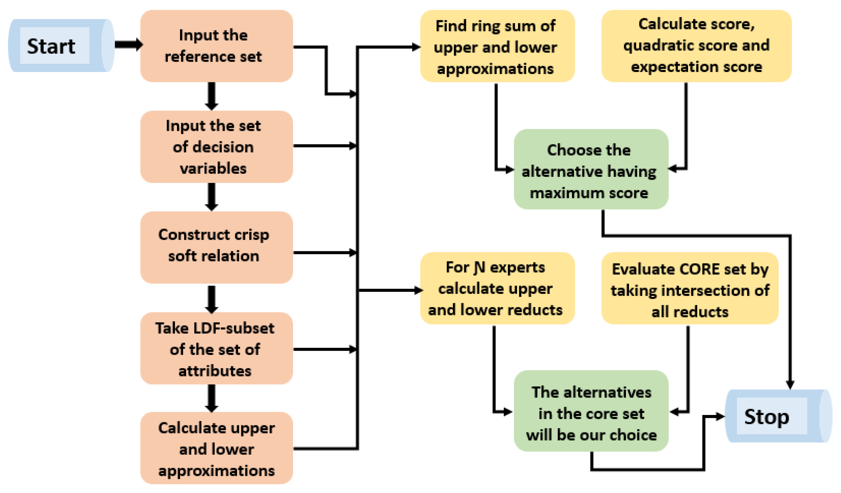
Algorithm 1: Selection of a best material handling equipment by using LDFSRSs.

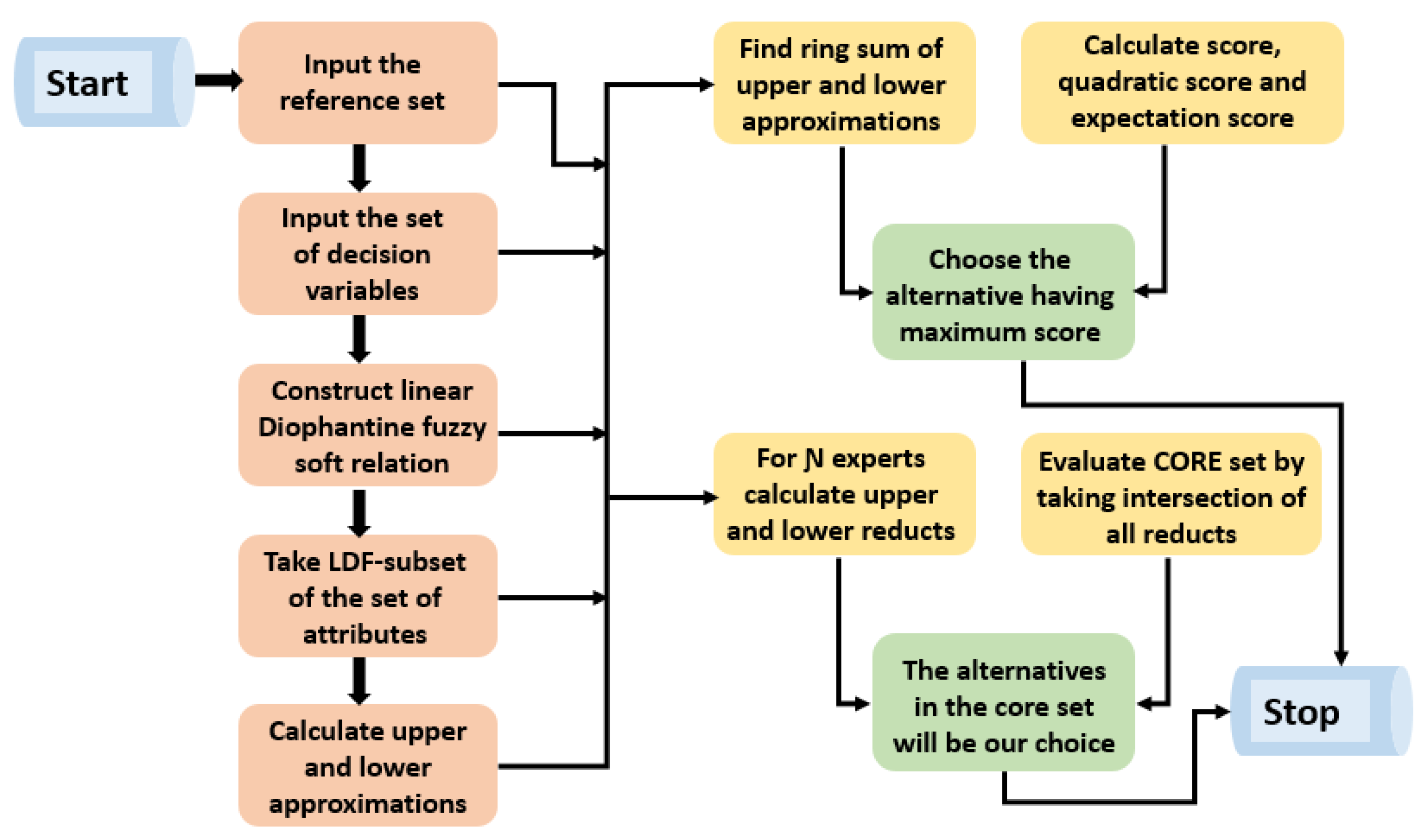
Input: 1. Input the reference set $\ddot{\mathcal{Q}}$. 2. Input the assembling of attributes $\dot{\mathcal{G}}$. Construction: 3. According to the necessity of the DM, build an LDFSR $\widetilde{ð}:\ddot{\mathcal{Q}}\to \dot{\mathcal{G}}$. 4. Based on the needs of the decision maker, construct LDF-subset ${\mathcal{B}}_{\mathcal{D}}$ of $\dot{\mathcal{G}}$ as an optimal normal decision set. Calculation: 5. Calculate the “LDFSR approximation operators” ${\widetilde{ð}}_{\divideontimes }\left({\mathcal{B}}_{\mathcal{D}}\right)$ and ${\widetilde{ð}}^{\divideontimes }\left({\mathcal{B}}_{\mathcal{D}}\right)$ as lower and upper using Definition 12. 6. By using Definition 13 of the ring sum operation, find the choice of LDFS ${\widetilde{ð}}_{\divideontimes }\left({\mathcal{B}}_{\mathcal{D}}\right)\oplus {\widetilde{ð}}^{\divideontimes }\left({\mathcal{B}}_{\mathcal{D}}\right)$. Output: 7. We use the definitions of score, quadratic score, and expectation score functions for LDFNs ${\ddot{\mathcal{A}}}_{\mathcal{D}}=(\langle {\dot{t}}_{\mathcal{D}},{\dot{f}}_{\mathcal{D}}\rangle ,\langle {\alpha }_{\mathcal{D}},{\beta }_{\mathcal{D}}\rangle )$ given in [54] and written respectively as: $${\mathcal{L}}_1\left({\ddot{\mathcal{A}}}_{\mathcal{D}}\right)=\frac{1}{2}[({\dot{t}}_{\mathcal{D}}-{\dot{f}}_{\mathcal{D}})+({\alpha }_{\mathcal{D}}-{\beta }_{\mathcal{D}})]$$ $${\mathcal{L}}_2\left({\ddot{\mathcal{A}}}_{\mathcal{D}}\right)=\frac{1}{2}[({\dot{t}}_{\mathcal{D}}^2-{\dot{f}}_{\mathcal{D}}^2)+({\alpha }_{\mathcal{D}}^2-{\beta }_{\mathcal{D}}^2)]$$ $${\mathcal{L}}_3\left({\ddot{\mathcal{A}}}_{\mathcal{D}}\right)=\frac{1}{2}[\frac{({\dot{t}}_{\mathcal{D}}-{\dot{f}}_{\mathcal{D}}+1)}{2}+\frac{({\alpha }_{\mathcal{D}}-{\beta }_{\mathcal{D}}+1)}{2}]$$ of every alternative in ${\widetilde{ð}}_{\divideontimes }\left({\mathcal{B}}_{\mathcal{D}}\right)\oplus {\widetilde{ð}}^{\divideontimes }\left({\mathcal{B}}_{\mathcal{D}}\right)$. 8. Rank the alternatives by using calculated score values. Final decision: 9. Choose the alternative having the maximum score value.

Algorithm 2: Selection of the best material handling equipment by using LDFSRSs.

Input: 1. Input the reference set $\ddot{\mathcal{Q}}$. 2. Input the assembling of attributes $\dot{\mathcal{G}}$. Construction: 3. According to the necessity of the DM, build an LDFSR $\widetilde{ð}:\ddot{\mathcal{Q}}\to \dot{\mathcal{G}}$. 4. Based on the needs of the decision maker, construct LDF-subset ${\mathcal{B}}_{\mathcal{D}}$ of $\dot{\mathcal{G}}$ as an optimal normal decision set. Calculation: 5. Calculate the “LDFSR approximation operators” ${\widetilde{ð}}_{\divideontimes }\left({\mathcal{B}}_{\mathcal{D}}\right)$ and ${\widetilde{ð}}^{\divideontimes }\left({\mathcal{B}}_{\mathcal{D}}\right)$ as lower and upper using Definition 12. 6. For “$\mathcal{N}$” number of experts, calculate upper and lower reducts from the calculated “upper and lower approximation operators”, respectively. Output: 7. From the calculated “$2\mathcal{N}$” reducts, we get “$2\mathcal{N}$” crisp subsets of the reference set $\ddot{\mathcal{Q}}$. The subsets can be constructed by using the “YES” and “NO” logic. The only alternatives in the reduct having final decision “YES” will become the object of the crisp subset. 8. Calculate the core set by taking the intersection of all crisp subsets obtained from the calculated reducts. Final decision: 9. The alternatives in the core will be our choice for the final decision.

4.1.1. Calculations by Using Algorithm 1

The indiscernibility relation is “the selection of best material handling equipment”. This relation can be observed by LDFSR, $\widetilde{ð}:\ddot{\mathcal{Q}}\to \dot{\mathcal{G}}$ given as

Table 11. LDFSR.

$\widetilde{\mathit{ð}}$	${\dot{\mathit{\wp }}}_1$	${\dot{\mathit{\wp }}}_2$	${\dot{\mathit{\wp }}}_3$	${\dot{\mathit{\wp }}}_4$
${\mathcal{G}}_1$	$(\langle 0.73,0.41\rangle ,\langle 0.31,0.13\rangle )$	$(\langle 0.63,0.53\rangle ,\langle 0.13,0.23\rangle )$	$(\langle 0.73,0.41\rangle ,\langle 0.23,0.15\rangle )$	$(\langle 0.63,0.53\rangle ,\langle 0.31,0.36\rangle )$
${\mathcal{G}}_2$	$(\langle 0.63,0.43\rangle ,\langle 0.41,0.42\rangle )$	$(\langle 0.74,0.32\rangle ,\langle 0.63,0.21\rangle )$	$(\langle 0.68,0.41\rangle ,\langle 0.53,0.21\rangle )$	$(\langle 0.71,0.41\rangle ,\langle 0.43,0.28\rangle )$
${\mathcal{G}}_3$	$(\langle 0.71,0.34\rangle ,\langle 0.51,0.31\rangle )$	$(\langle 0.63,0.51\rangle ,\langle 0.43,0.39\rangle )$	$(\langle 0.71,0.41\rangle ,\langle 0.31,0.41\rangle )$	$(\langle 0.69,0.38\rangle ,\langle 0.41,0.31\rangle )$
${\mathcal{G}}_4$	$(\langle 0.69,0.59\rangle ,\langle 0.61,0.21\rangle )$	$(\langle 0.81,0.51\rangle ,\langle 0.31,0.42\rangle )$	$(\langle 0.83,0.41\rangle ,\langle 0.32,0.41\rangle )$	$(\langle 0.73,0.49\rangle ,\langle 0.41,0.21\rangle )$
${\mathcal{G}}_5$	$(\langle 0.72,0.41\rangle ,\langle 0.51,0.21\rangle )$	$(\langle 0.83,0.41\rangle ,\langle 0.42,0.31\rangle )$	$(\langle 0.73,0.41\rangle ,\langle 0.31,0.42\rangle )$	$(\langle 0.83,0.49\rangle ,\langle 0.28,0.41\rangle )$
${\mathcal{G}}_6$	$(\langle 0.63,0.59\rangle ,\langle 0.41,0.31\rangle )$	$(\langle 0.78,0.43\rangle ,\langle 0.38,0.41\rangle )$	$(\langle 0.63,0.48\rangle ,\langle 0.28,0.17\rangle )$	$(\langle 0.58,0.49\rangle ,\langle 0.31,0.42\rangle )$
${\mathcal{G}}_7$	$(\langle 0.81,0.58\rangle ,\langle 0.49,0.31\rangle )$	$(\langle 0.73,0.68\rangle ,\langle 0.43,0.49\rangle )$	$(\langle 0.69,0.73\rangle ,\langle 0.31,0.31\rangle )$	$(\langle 0.68,0.51\rangle ,\langle 0.43,0.21\rangle )$

.

Thus, $\widetilde{ð}$ is an LDFSR on $\ddot{\mathcal{Q}}\times \dot{\mathcal{G}}$. This relation gives us the numeric values in the form of LDFNs of each alternative corresponding to every decision variable. For example, for the alternative ${\mathcal{G}}_1$, the decision variable ${\dot{\wp }}_1$ (“Technical: convenience, maintainability, safety required”) has numeric value $(\langle 0.73,0.41\rangle ,\langle 0.31,0.13\rangle )$. This value shows that the alternative ${\mathcal{G}}_1$ is $73\%$ technical and $41\%$ has a falsity value for technicality. The pair $\langle 0.31,0.13\rangle$ represents the reference parameters for the truth and falsity grades, where we can observe that alternative ${\mathcal{G}}_1$ is $31\%$ highly technical and it has $13\%$ low technicality. These sub-criteria for the alternatives can be observed from Table 10. All the remaining values can be constructed according to a similar pattern. We consider that experts give some opinion about the attributes and rank them according to their requirement. We convert the verbal description into the LDFS numeric values in the form of LDFS ${\mathcal{B}}_{\mathcal{D}}$. The set ${\mathcal{B}}_{\mathcal{D}}$ is the LDF-subset of $\dot{\mathcal{G}}$ and written as follows:

$$\begin{array}{c}\hfill {\mathcal{B}}_{\mathcal{D}}=\{({\dot{\wp }}_1,\langle 00.63,00.41\rangle ,\langle 00.31,00.33\rangle ),({\dot{\wp }}_2,\langle 00.71,00.51\rangle ,\langle 00.41,00.38\rangle ),\\ \hfill ({\dot{\wp }}_3,\langle 00.75,00.63\rangle ,\langle 00.51,00.32\rangle ),({\dot{\wp }}_4,\langle 00.83,00.51\rangle ,\langle 00.41,00.21\rangle )\}.\end{array}$$

We evaluate the “lower and upper approximations” of LDFS ${\mathcal{B}}_{\mathcal{D}}$ on LDFSR $\widetilde{ð}$.

$$\begin{array}{cc}\hfill {\widetilde{ð}}^{\divideontimes }\left({\mathcal{B}}_{\mathcal{D}}\right)& =\{({\mathcal{G}}_1,\langle 00.73,00.51\rangle ,\langle 00.31,00.64\rangle ),({\mathcal{G}}_2,\langle 00.71,00.57\rangle ,\langle 00.51,00.58\rangle ),({\mathcal{G}}_3,\langle 00.71,00.51\rangle ,\langle 00.41,00.59\rangle ),\hfill \\ \hfill & ({\mathcal{G}}_4,\langle 00.75,00.41\rangle ,\langle 00.41,00.58\rangle ),({\mathcal{G}}_5,\langle 00.83,00.51\rangle ,\langle 00.41,00.58\rangle ,({\mathcal{G}}_6,\langle 00.71,00.41\rangle ,\langle 00.38,00.58\rangle ,\hfill \\ \hfill & ({\mathcal{G}}_7,\langle 00.71,00.42\rangle ,\langle 00.41,00.51\rangle )\}\hfill \\ \hfill {\widetilde{ð}}_{\divideontimes }\left({\mathcal{B}}_{\mathcal{D}}\right)& =\{({\mathcal{G}}_1,\langle 00.63,00.51\rangle ,\langle 00.69,00.23\rangle ),({\mathcal{G}}_2,\langle 00.63,00.41\rangle ,\langle 00.41,00.33\rangle ),({\mathcal{G}}_3,\langle 00.63,00.51\rangle ,\langle 00.49,00.38\rangle ),\hfill \\ \hfill & ({\mathcal{G}}_4,\langle 00.63,00.51\rangle ,\langle 00.39,00.38\rangle ),({\mathcal{G}}_5,\langle 00.63,00.49\rangle ,\langle 00.49,00.32\rangle ,({\mathcal{G}}_6,\langle 00.63,00.49\rangle ,\langle 00.59,00.38\rangle ,\hfill \\ \hfill & ({\mathcal{G}}_7,\langle 00.63,00.63\rangle ,\langle 00.51,00.38\rangle )\}\hfill \end{array}$$

$$\begin{array}{cc}\hfill {\widetilde{ð}}_{\divideontimes }\left({\mathcal{B}}_{\mathcal{D}}\right)\oplus {\widetilde{ð}}^{\divideontimes }\left({\mathcal{B}}_{\mathcal{D}}\right)& =\{({\mathcal{G}}_1,\langle 0.900,0.260\rangle ,\langle 0.780,0.140\rangle ),({\mathcal{G}}_2,\langle 0.890,0.230\rangle ,\langle 0.710,0.190\rangle ),\hfill \\ \hfill & ({\mathcal{G}}_3,\langle 0.890,0.260\rangle ,\langle 0.690,0.220\rangle ),({\mathcal{G}}_4,\langle 0.900,0.200\rangle ,\langle 0.640,0.220\rangle ),\hfill \\ \hfill & ({\mathcal{G}}_5,\langle 0.937,0.249\rangle ,\langle 0.699,0.185\rangle ,({\mathcal{G}}_6,\langle 0.892,0.200\rangle ,\langle 0.745,0.220\rangle ,\hfill \\ \hfill & ({\mathcal{G}}_7,\langle 0.890,0.260\rangle ,\langle 0.710,0.190\rangle )\}\hfill \end{array}$$

Now, we calculate the score values, quadratic score values, and expectation score values of the alternatives in ${\widetilde{ð}}_{\divideontimes }\left({\mathcal{B}}_{\mathcal{D}}\right)\oplus {\widetilde{ð}}^{\divideontimes }\left({\mathcal{B}}_{\mathcal{D}}\right)$. The final ranking is given in

Table 12. Ranking of alternatives for different score values.

LDFS	${\mathcal{G}}_1$	${\mathcal{G}}_2$	${\mathcal{G}}_3$	${\mathcal{G}}_4$	${\mathcal{G}}_5$	${\mathcal{G}}_6$	${\mathcal{G}}_7$	Ranking	Final Decision
${\mathcal{L}}_1$ (SF)	$0.640$	$0.590$	$0.550$	$0.560$	$0.601$	$0.608$	$0.575$	${\mathcal{G}}_1\succ {\mathcal{G}}_6\succ {\mathcal{G}}_5\succ {\mathcal{G}}_2\succ {\mathcal{G}}_7\succ {\mathcal{G}}_4\succ {\mathcal{G}}_3$	${\mathcal{G}}_1$
${\mathcal{L}}_2$ (QSF)	$0.665$	$0.603$	$0.576$	$0.565$	$0.635$	$0.631$	$0.596$	${\mathcal{G}}_1\succ {\mathcal{G}}_5\succ {\mathcal{G}}_6\succ {\mathcal{G}}_2\succ {\mathcal{G}}_7\succ {\mathcal{G}}_3\succ {\mathcal{G}}_4$	${\mathcal{G}}_1$
${\mathcal{L}}_3$ (ESF)	$0.820$	$0.795$	$0.775$	$0.780$	$0.800$	$0.804$	$0.787$	${\mathcal{G}}_1\succ {\mathcal{G}}_6\succ {\mathcal{G}}_5\succ {\mathcal{G}}_2\succ {\mathcal{G}}_7\succ {\mathcal{G}}_4\succ {\mathcal{G}}_3$	${\mathcal{G}}_1$

.

From Table 12, we can observe that the alternative ${\mathcal{G}}_1$ is most suitable for the final decision. The bar chart of the ranking results for alternatives is given in Figure 4.

4.1.2. Calculations by Using Algorithm 2

In Algorithm 1, we use the input data in the form of linguistic terms as LDFNs. We only deal with the truth and falsity grades with their reference parameters, and we have no idea about the expert’s opinion. Due to the lack of information, we have some uncertainty in our decision. This uncertainty can be removed by giving some weight to the expert’s opinion. Therefore, we establish upper and lower reducts for all the experts one by one. The initial five steps of Algorithm 2 are the same as Algorithm 1. We will proceed next by constructing the upper and lower reducts from “upper and lower approximations” of LDFS for all the experts. Suppose that we have three experts from the company’s technical committee given as:

$$\begin{array}{c}\hfill \mathrm{Expert}\mathrm{X}\\ \hfill \mathrm{Expert}\mathrm{Y}\\ \hfill \mathrm{Expert}\mathrm{Z}\end{array}$$

The reducts from approximations can be constructed by using the following terms.

$$\begin{array}{cc}\hfill {\ddot{\mathcal{T}}}_{\mathcal{D}}& =\mathrm{Truth}\mathrm{membership}\mathrm{grade},\hfill \\ \hfill {\ddot{\mathcal{S}}}_{\mathcal{D}}& =\mathrm{Falsity}\mathrm{membership}\mathrm{grade},\hfill \\ \hfill {\alpha }_{\mathcal{D}}& =\mathrm{Reference}\mathrm{parameter}\mathrm{corresponding}\mathrm{to}\mathrm{truth}\mathrm{membership}\mathrm{grade},\hfill \\ \hfill {\beta }_{\mathcal{D}}& =\mathrm{Reference}\mathrm{parameter}\mathrm{corresponding}\mathrm{to}\mathrm{falsity}\mathrm{membership}\mathrm{grade},\hfill \\ \hfill {\mathcal{L}}_3& =\mathrm{Expectation}\mathrm{score}\mathrm{function}\mathrm{value}\mathrm{of}\mathrm{LDFN},\hfill \\ \hfill \widehat{\mathcal{L}}& =\mathrm{Ranking}\mathrm{given}\mathrm{by}\mathrm{experts}\mathrm{to}\mathrm{the}\mathrm{alternatives}\mathrm{from}\mathrm{crisp}\mathrm{set}\{0,1\},\hfill \\ \hfill {\mathcal{L}}^{*}& =\mathrm{Selection}\mathrm{of}\mathrm{alternative}\mathrm{by}\mathrm{using}‘‘\mathrm{YES}’’\mathrm{or}‘‘\mathrm{NO}’’,\mathrm{i}.\mathrm{e}.,\mathrm{take}\mathrm{average}\mathrm{of}\hfill \\ \hfill & \mathrm{scores}{\mathcal{L}}_3\mathrm{for}\mathrm{all}\mathrm{the}\mathrm{alternatives}.\mathrm{The}\mathrm{alternatives}\mathrm{that}\mathrm{have}\mathrm{a}\mathrm{grater}\hfill \\ \hfill & \mathrm{or}\mathrm{equal}\mathrm{score}{\mathcal{L}}_3\mathrm{than}/\mathrm{to}\mathrm{the}\mathrm{average}\mathrm{can}\mathrm{be}\mathrm{seleted}\mathrm{as}‘‘\mathrm{YES}’’;\mathrm{those}\mathrm{who}\hfill \\ \hfill & \mathrm{have}\mathrm{a}\mathrm{lesser}\mathrm{score}\mathrm{than}\mathrm{the}\mathrm{average}\mathrm{value}\mathrm{can}\mathrm{be}\mathrm{neglected}\mathrm{as}‘‘\mathrm{NO}’’,\hfill \\ \hfill F.D& =\mathrm{Fianl}\mathrm{decision}\hfill \end{array}$$

The final decision is based on $\widehat{\mathcal{L}}$ and ${\mathcal{L}}^{*}$ given in

Table 13. The criteria for the final decision (F.D).

$\widehat{\mathcal{L}}$	${\mathcal{L}}^{*}$	F.D
0	NO	NO
1	YES	YES
0	YES	NO
1	NO	NO

.

For expert-X, the upper reduct of upper approximation ${\widetilde{ð}}^{\divideontimes }\left({\mathcal{B}}_{\mathcal{D}}\right)$ (calculated in Algorithm 1) of LDFS ${\mathcal{B}}_{\mathcal{D}}$ is given as

Table 14. Upper reduct for expert-X $\left(U_X\right)$ from ${\widetilde{ð}}^{\divideontimes }\left({\mathcal{B}}_{\mathcal{D}}\right)$.

$\left({\mathit{U}}_{\mathit{X}}\right)$	${\ddot{\mathcal{T}}}_{\mathcal{D}}$	${\ddot{\mathcal{S}}}_{\mathcal{D}}$	${\mathit{\alpha }}_{\mathcal{D}}$	${\mathit{\beta }}_{\mathcal{D}}$	${\mathcal{L}}_3$	$\widehat{\mathcal{L}}$	${\mathcal{L}}^{*}$	F.D
${\mathcal{G}}_1$	$0.73$	$0.51$	$0.31$	$0.64$	$0.472$	1	${\mathcal{L}}_3<0.520\to$ NO	NO
${\mathcal{G}}_2$	$0.71$	$0.57$	$0.51$	$0.58$	$0.517$	0	${\mathcal{L}}_3<0.520\to$ NO	NO
${\mathcal{G}}_3$	$0.71$	$0.51$	$0.41$	$0.59$	$0.505$	1	${\mathcal{L}}_3<0.520\to$ NO	NO
${\mathcal{G}}_4$	$0.75$	$0.41$	$0.41$	$0.58$	$0.542$	0	${\mathcal{L}}_3>0.520\to$ YES	NO
${\mathcal{G}}_5$	$0.83$	$0.51$	$0.41$	$0.58$	$0.537$	1	${\mathcal{L}}_3>0.520\to$ YES	YES
${\mathcal{G}}_6$	$0.71$	$0.41$	$0.38$	$0.58$	$0.525$	1	${\mathcal{L}}_3>0.520\to$ YES	YES
${\mathcal{G}}_7$	$0.71$	$0.42$	$0.41$	$0.51$	$0.547$	1	${\mathcal{L}}_3>0.520\to$ YES	YES

. The average of the score values of all the alternatives for ${\widetilde{ð}}^{\divideontimes }\left({\mathcal{B}}_{\mathcal{D}}\right)$ is $0.520$.

This implies that $U_X=\{{\mathcal{G}}_5,{\mathcal{G}}_6,{\mathcal{G}}_7\}$. For expert-X, the lower reduct of lower approximation ${\widetilde{ð}}_{\divideontimes }\left({\mathcal{B}}_{\mathcal{D}}\right)$ (calculated in Algorithm 1) of LDFS ${\mathcal{B}}_{\mathcal{D}}$ is given as

Table 15. Lower reduct for expert-X $\left(L_X\right)$ from ${\widetilde{ð}}^{\divideontimes }\left({\mathcal{B}}_{\mathcal{D}}\right)$.

$\left({\mathit{L}}_{\mathit{X}}\right)$	${\ddot{\mathcal{T}}}_{\mathcal{D}}$	${\ddot{\mathcal{S}}}_{\mathcal{D}}$	${\mathit{\alpha }}_{\mathcal{D}}$	${\mathit{\beta }}_{\mathcal{D}}$	${\mathcal{L}}_3$	$\widehat{\mathcal{L}}$	${\mathcal{L}}^{*}$	F.D
${\mathcal{G}}_1$	$0.63$	$0.51$	$0.69$	$0.23$	$0.645$	1	${\mathcal{L}}_3>0.572\to$ YES	YES
${\mathcal{G}}_2$	$0.63$	$0.41$	$0.41$	$0.33$	$0.575$	0	${\mathcal{L}}_3>0.572\to$ YES	NO
${\mathcal{G}}_3$	$0.63$	$0.51$	$0.49$	$0.38$	$0.557$	1	${\mathcal{L}}_3<0.572\to$ NO	NO
${\mathcal{G}}_4$	$0.63$	$0.51$	$0.39$	$0.38$	$0.532$	0	${\mathcal{L}}_3<0.572\to$ NO	NO
${\mathcal{G}}_5$	$0.63$	$0.49$	$0.49$	$0.32$	$0.577$	1	${\mathcal{L}}_3>0.572\to$ YES	YES
${\mathcal{G}}_6$	$0.63$	$0.49$	$0.59$	$0.38$	$0.587$	1	${\mathcal{L}}_3>0.572\to$ YES	YES
${\mathcal{G}}_7$	$0.63$	$0.63$	$0.51$	$0.38$	$0.532$	1	${\mathcal{L}}_3<0.572\to$ NO	NO

. The average of the score values of all the alternatives for ${\widetilde{ð}}_{\divideontimes }\left({\mathcal{B}}_{\mathcal{D}}\right)$ is $0.572$.

This implies that $L_X=\{{\mathcal{G}}_1,{\mathcal{G}}_5,{\mathcal{G}}_6\}$. For expert-Y, the upper reduct of upper approximation ${\widetilde{ð}}^{\divideontimes }\left({\mathcal{B}}_{\mathcal{D}}\right)$ (calculated in Algorithm 1) of LDFS ${\mathcal{B}}_{\mathcal{D}}$ is given as

Table 16. Upper reduct for expert-Y $\left(U_Y\right)$ from ${\widetilde{ð}}^{\divideontimes }\left({\mathcal{B}}_{\mathcal{D}}\right)$.

$\left({\mathit{U}}_{\mathit{Y}}\right)$	${\ddot{\mathcal{T}}}_{\mathcal{D}}$	${\ddot{\mathcal{S}}}_{\mathcal{D}}$	${\mathit{\alpha }}_{\mathcal{D}}$	${\mathit{\beta }}_{\mathcal{D}}$	${\mathcal{L}}_3$	$\widehat{\mathcal{L}}$	${\mathcal{L}}^{*}$	F.D
${\mathcal{G}}_1$	$0.73$	$0.51$	$0.31$	$0.64$	$0.472$	0	${\mathcal{L}}_3<0.520\to$ NO	NO
${\mathcal{G}}_2$	$0.71$	$0.57$	$0.51$	$0.58$	$0.517$	1	${\mathcal{L}}_3<0.520\to$ NO	NO
${\mathcal{G}}_3$	$0.71$	$0.51$	$0.41$	$0.59$	$0.505$	0	${\mathcal{L}}_3<0.520\to$ NO	NO
${\mathcal{G}}_4$	$0.75$	$0.41$	$0.41$	$0.58$	$0.542$	1	${\mathcal{L}}_3>0.520\to$ YES	YES
${\mathcal{G}}_5$	$0.83$	$0.51$	$0.41$	$0.58$	$0.537$	1	${\mathcal{L}}_3>0.520\to$ YES	YES
${\mathcal{G}}_6$	$0.71$	$0.41$	$0.38$	$0.58$	$0.525$	1	${\mathcal{L}}_3>0.520\to$ YES	YES
${\mathcal{G}}_7$	$0.71$	$0.42$	$0.41$	$0.51$	$0.547$	0	${\mathcal{L}}_3>0.520\to$ YES	NO

. The average of the score values of all the alternatives for ${\widetilde{ð}}^{\divideontimes }\left({\mathcal{B}}_{\mathcal{D}}\right)$ is $0.520$.

This implies that $U_Y=\{{\mathcal{G}}_4,{\mathcal{G}}_5,{\mathcal{G}}_6\}$. For expert-Y, the lower reduct of lower approximation ${\widetilde{ð}}_{\divideontimes }\left({\mathcal{B}}_{\mathcal{D}}\right)$ (calculated in Algorithm 1) of LDFS ${\mathcal{B}}_{\mathcal{D}}$ is given as

Table 17. Lower reduct for expert-Y $\left(L_Y\right)$ from ${\widetilde{ð}}^{\divideontimes }\left({\mathcal{B}}_{\mathcal{D}}\right)$.

$\left({\mathit{L}}_{\mathit{Y}}\right)$	${\ddot{\mathcal{T}}}_{\mathcal{D}}$	${\ddot{\mathcal{S}}}_{\mathcal{D}}$	${\mathit{\alpha }}_{\mathcal{D}}$	${\mathit{\beta }}_{\mathcal{D}}$	${\mathcal{L}}_3$	$\widehat{\mathcal{L}}$	${\mathcal{L}}^{*}$	F.D
${\mathcal{G}}_1$	$0.63$	$0.51$	$0.69$	$0.23$	$0.645$	0	${\mathcal{L}}_3>0.572\to$ YES	NO
${\mathcal{G}}_2$	$0.63$	$0.41$	$0.41$	$0.33$	$0.575$	1	${\mathcal{L}}_3>0.572\to$ YES	YES
${\mathcal{G}}_3$	$0.63$	$0.51$	$0.49$	$0.38$	$0.557$	0	${\mathcal{L}}_3<0.572\to$ NO	NO
${\mathcal{G}}_4$	$0.63$	$0.51$	$0.39$	$0.38$	$0.532$	1	${\mathcal{L}}_3<0.572\to$ NO	NO
${\mathcal{G}}_5$	$0.63$	$0.49$	$0.49$	$0.32$	$0.577$	1	${\mathcal{L}}_3>0.572\to$ YES	YES
${\mathcal{G}}_6$	$0.63$	$0.49$	$0.59$	$0.38$	$0.587$	1	${\mathcal{L}}_3>0.572\to$ YES	YES
${\mathcal{G}}_7$	$0.63$	$0.63$	$0.51$	$0.38$	$0.532$	0	${\mathcal{L}}_3<0.572\to$ NO	NO

. The average of the score values of all the alternatives for ${\widetilde{ð}}_{\divideontimes }\left({\mathcal{B}}_{\mathcal{D}}\right)$ is $0.572$.

This implies that $L_Y=\{{\mathcal{G}}_2,{\mathcal{G}}_5,{\mathcal{G}}_6\}$. For expert-Z, the upper reduct of upper approximation ${\widetilde{ð}}^{\divideontimes }\left({\mathcal{B}}_{\mathcal{D}}\right)$ (calculated in Algorithm 1) of LDFS ${\mathcal{B}}_{\mathcal{D}}$ is given as

Table 18. Upper reduct for expert-Z $\left(U_Z\right)$ from ${\widetilde{ð}}^{\divideontimes }\left({\mathcal{B}}_{\mathcal{D}}\right)$.

$\left({\mathit{U}}_{\mathit{Y}}\right)$	${\ddot{\mathcal{T}}}_{\mathcal{D}}$	${\ddot{\mathcal{S}}}_{\mathcal{D}}$	${\mathit{\alpha }}_{\mathcal{D}}$	${\mathit{\beta }}_{\mathcal{D}}$	${\mathcal{L}}_3$	$\widehat{\mathcal{L}}$	${\mathcal{L}}^{*}$	F.D
${\mathcal{G}}_1$	$0.73$	$0.51$	$0.31$	$0.64$	$0.472$	1	${\mathcal{L}}_3<0.520\to$ NO	NO
${\mathcal{G}}_2$	$0.71$	$0.57$	$0.51$	$0.58$	$0.517$	1	${\mathcal{L}}_3<0.520\to$ NO	NO
${\mathcal{G}}_3$	$0.71$	$0.51$	$0.41$	$0.59$	$0.505$	0	${\mathcal{L}}_3<0.520\to$ NO	NO
${\mathcal{G}}_4$	$0.75$	$0.41$	$0.41$	$0.58$	$0.542$	0	${\mathcal{L}}_3>0.520\to$ YES	NO
${\mathcal{G}}_5$	$0.83$	$0.51$	$0.41$	$0.58$	$0.537$	1	${\mathcal{L}}_3>0.520\to$ YES	YES
${\mathcal{G}}_6$	$0.71$	$0.41$	$0.38$	$0.58$	$0.525$	0	${\mathcal{L}}_3>0.520\to$ YES	NO
${\mathcal{G}}_7$	$0.71$	$0.42$	$0.41$	$0.51$	$0.547$	1	${\mathcal{L}}_3>0.520\to$ YES	YES

. The average of the score values of all the alternatives for ${\widetilde{ð}}^{\divideontimes }\left({\mathcal{B}}_{\mathcal{D}}\right)$ is $0.520$.

This implies that $U_Z=\{{\mathcal{G}}_5,{\mathcal{G}}_7\}$. For expert-Z, the lower reduct of lower approximation ${\widetilde{ð}}_{\divideontimes }\left({\mathcal{B}}_{\mathcal{D}}\right)$ (calculated in Algorithm 1) of LDFS ${\mathcal{B}}_{\mathcal{D}}$ is given as

Table 19. Lower reduct for expert-Z $\left(L_Z\right)$ from ${\widetilde{ð}}^{\divideontimes }\left({\mathcal{B}}_{\mathcal{D}}\right)$.

$\left({\mathit{L}}_{\mathit{Z}}\right)$	${\ddot{\mathcal{T}}}_{\mathcal{D}}$	${\ddot{\mathcal{S}}}_{\mathcal{D}}$	${\mathit{\alpha }}_{\mathcal{D}}$	${\mathit{\beta }}_{\mathcal{D}}$	${\mathcal{L}}_3$	$\widehat{\mathcal{L}}$	${\mathcal{L}}^{*}$	F.D
${\mathcal{G}}_1$	$0.63$	$0.51$	$0.69$	$0.23$	$0.645$	1	${\mathcal{L}}_3>0.572\to$ YES	YES
${\mathcal{G}}_2$	$0.63$	$0.41$	$0.41$	$0.33$	$0.575$	1	${\mathcal{L}}_3>0.572\to$ YES	YES
${\mathcal{G}}_3$	$0.63$	$0.51$	$0.49$	$0.38$	$0.557$	0	${\mathcal{L}}_3<0.572\to$ NO	NO
${\mathcal{G}}_4$	$0.63$	$0.51$	$0.39$	$0.38$	$0.532$	0	${\mathcal{L}}_3<0.572\to$ NO	NO
${\mathcal{G}}_5$	$0.63$	$0.49$	$0.49$	$0.32$	$0.577$	1	${\mathcal{L}}_3>0.572\to$ YES	YES
${\mathcal{G}}_6$	$0.63$	$0.49$	$0.59$	$0.38$	$0.587$	0	${\mathcal{L}}_3>0.572\to$ YES	NO
${\mathcal{G}}_7$	$0.63$	$0.63$	$0.51$	$0.38$	$0.532$	1	${\mathcal{L}}_3<0.572\to$ NO	NO

. The average of the score values of all the alternatives for ${\widetilde{ð}}_{\divideontimes }\left({\mathcal{B}}_{\mathcal{D}}\right)$ is $0.572$.

This implies that $L_Z=\{{\mathcal{G}}_1,{\mathcal{G}}_2,{\mathcal{G}}_5\}$. Now, we calculate the core set by taking the intersection of all upper and lower reducts for all three experts.

$$\mathrm{core}=U_X\cap L_X\cap U_Y\cap L_Y\cap U_Z\cap L_Z=\left\{{\mathcal{G}}_5\right\}$$

This means that “${\mathcal{G}}_5$” is the most suitable alternative for the final decision.

4.2. Selection of the Most Appropriate Material Handling Equipment by Using SRLDFSs

Now, we use our second novel structure of SRLDFS and “crisp soft approximation space” for the selection of the most appropriate material handling equipment. We construct two novel algorithms (Algorithms 3 and 4) for the selection. The flowchart diagram of both algorithms is given in Figure 5.

Algorithm 3: Selection of the best material handling equipment by using SRLDFSs.

Input: 1. Input the reference set $\ddot{\mathcal{Q}}$. 2. Input the assembling of attributes $\dot{\mathcal{G}}$. Construction: 3. According to the necessity of the DM, build a crisp soft relation $\tilde{\mathcal{A}}$ over $\ddot{\mathcal{Q}}\times \dot{\mathcal{G}}$. 4. Based on the needs of the decision maker, construct LDF-subset $\mathcal{H}$ of $\dot{\mathcal{G}}$ as an optimal normal decision set. Calculation: 5. Calculate the “SRLDF approximation operators” ${\tilde{\mathcal{A}}}_{\divideontimes }\left(\mathcal{H}\right)$ and ${\tilde{\mathcal{A}}}^{\divideontimes }\left(\mathcal{H}\right)$ as “lower and upper approximations” by using Definition 9. 6. By using Definition 13 of the ring sum operation, find the choice of LDFS ${\tilde{\mathcal{A}}}_{\divideontimes }\left(\mathcal{H}\right)\oplus {\tilde{\mathcal{A}}}^{\divideontimes }\left(\mathcal{H}\right)$. Output: 7. We use the definitions of the score, quadratic score, and expectation score functions for LDFNs ${\ddot{\mathcal{A}}}_{\mathcal{D}}=(\langle {\dot{t}}_{\mathcal{D}},{\dot{f}}_{\mathcal{D}}\rangle ,\langle {\alpha }_{\mathcal{D}},{\beta }_{\mathcal{D}}\rangle )$ given in [54] and written respectively as: $${\mathcal{L}}_1\left({\ddot{\mathcal{A}}}_{\mathcal{D}}\right)=\frac{1}{2}[({\dot{t}}_{\mathcal{D}}-{\dot{f}}_{\mathcal{D}})+({\alpha }_{\mathcal{D}}-{\beta }_{\mathcal{D}})]$$ $${\mathcal{L}}_2\left({\ddot{\mathcal{A}}}_{\mathcal{D}}\right)=\frac{1}{2}[({\dot{t}}_{\mathcal{D}}^2-{\dot{f}}_{\mathcal{D}}^2)+({\alpha }_{\mathcal{D}}^2-{\beta }_{\mathcal{D}}^2)]$$ $${\mathcal{L}}_3\left({\ddot{\mathcal{A}}}_{\mathcal{D}}\right)=\frac{1}{2}[\frac{({\dot{t}}_{\mathcal{D}}-{\dot{f}}_{\mathcal{D}}+1)}{2}+\frac{({\alpha }_{\mathcal{D}}-{\beta }_{\mathcal{D}}+1)}{2}]$$ of every alternative in ${\tilde{\mathcal{A}}}_{\divideontimes }\left(\mathcal{H}\right)\oplus {\tilde{\mathcal{A}}}^{\divideontimes }\left(\mathcal{H}\right)$. 8. Rank the alternatives by using calculated score values. Final decision: 9. Select the object having the highest score value.

Algorithm 4: Selection of the best material handling equipment by using SRLDFSs.

Input: 1. Input the reference set $\ddot{\mathcal{Q}}$. 2. Input the assembling of attributes $\dot{\mathcal{G}}$. Construction: 3. According to the necessity of the DM, build a crisp soft relation $\tilde{\mathcal{A}}$ over $\ddot{\mathcal{Q}}\times \dot{\mathcal{G}}$. 4. Based on the needs of the decision maker, construct LDF-subset $\mathcal{H}$ of $\dot{\mathcal{G}}$ as an optimal normal decision set. Calculation: 5. Calculate the “SRLDF approximation operators” ${\tilde{\mathcal{A}}}_{\divideontimes }\left(\mathcal{H}\right)$ and ${\tilde{\mathcal{A}}}^{\divideontimes }\left(\mathcal{H}\right)$ as “lower and upper approximations” by using Definition 9. 6. For “$\mathcal{N}$” number of experts, calculate upper and lower reducts from the calculated “upper and lower approximation operators”, respectively. Output: 7. From calculated “$2\mathcal{N}$” reducts, we get “$2\mathcal{N}$” crisp subsets of the reference set $\ddot{\mathcal{Q}}$. The subsets can be constructed by using the “YES” and “NO” logic. The only alternatives in the reduct having final decision “YES” will become the object of the crisp subset. 8. Calculate the core set by taking the intersection of all crisp subsets obtained from the calculated reducts. Final decision: 9. The alternatives in the core will be our choice for the final decision.

4.2.1. Calculations by Using Algorithm 3

We consider the indiscernibility relation “selection of best material handling equipment”. This relation is represented as a crisp soft relation $\tilde{\mathcal{A}}$ over $\ddot{\mathcal{Q}}\times \dot{\mathcal{G}}$ given as

Table 20. Crisp soft relation $\tilde{\mathcal{A}}$.

$\tilde{\mathcal{A}}$	${\dot{\mathit{\wp }}}_1$	${\dot{\mathit{\wp }}}_2$	${\dot{\mathit{\wp }}}_3$	${\dot{\mathit{\wp }}}_4$
${\mathcal{G}}_1$	0	0	1	1
${\mathcal{G}}_2$	0	1	1	0
${\mathcal{G}}_3$	1	1	0	0
${\mathcal{G}}_4$	1	1	1	0
${\mathcal{G}}_5$	1	1	0	1
${\mathcal{G}}_6$	1	0	0	1
${\mathcal{G}}_7$	0	1	1	0

.

Thus, $\tilde{\mathcal{A}}$ over $\ddot{\mathcal{Q}}\times \dot{\mathcal{G}}$ is a crisp soft relation. Table 20 shows that we have:

$$\begin{array}{cc}\hfill {\tilde{\mathcal{A}}}_s\left({\mathcal{G}}_1\right)& =\{{\dot{\wp }}_3,{\dot{\wp }}_4\}\hfill \\ \hfill {\tilde{\mathcal{A}}}_s\left({\mathcal{G}}_2\right)& =\{{\dot{\wp }}_2,{\dot{\wp }}_3\}\hfill \\ \hfill {\tilde{\mathcal{A}}}_s\left({\mathcal{G}}_3\right)& =\{{\dot{\wp }}_1,{\dot{\wp }}_2\}\hfill \\ \hfill {\tilde{\mathcal{A}}}_s\left({\mathcal{G}}_4\right)& =\{{\dot{\wp }}_1,{\dot{\wp }}_2,{\dot{\wp }}_3\}\hfill \\ \hfill {\tilde{\mathcal{A}}}_s\left({\mathcal{G}}_5\right)& =\{{\dot{\wp }}_1,{\dot{\wp }}_2,{\dot{\wp }}_4\}\hfill \\ \hfill {\tilde{\mathcal{A}}}_s\left({\mathcal{G}}_6\right)& =\{{\dot{\wp }}_1,{\dot{\wp }}_4\}\hfill \\ \hfill {\tilde{\mathcal{A}}}_s\left({\mathcal{G}}_7\right)& =\{{\dot{\wp }}_2,{\dot{\wp }}_3\}\hfill \end{array}$$

We consider that experts give some opinion about the attributes and rank them according to their requirements. We convert the verbal description into the LDFS numeric values in the form of LDFS $\mathcal{H}$. The set $\mathcal{H}$ is the LDF-subset of $\dot{\mathcal{G}}$ and written as follows:

$$\begin{array}{c}\hfill \mathcal{H}=\{({\dot{\wp }}_1,\langle 0.63,0.41\rangle ,\langle 0.31,0.33\rangle ),({\dot{\wp }}_2,\langle 0.71,0.51\rangle ,\langle 0.41,0.38\rangle ),\\ \hfill ({\dot{\wp }}_3,\langle 0.75,0.63\rangle ,\langle 0.51,0.32\rangle ),({\dot{\wp }}_4,\langle 0.83,0.51\rangle ,\langle 0.41,0.21\rangle )\}.\end{array}$$

Now, we find “upper and lower approximations” of set $\mathcal{H}$ over the relation $\tilde{\mathcal{A}}$ by using Definition 9 given as:

$$\begin{array}{cc}\hfill {\tilde{\mathcal{A}}}^{\divideontimes }\left(\mathcal{H}\right)& =\{({\mathcal{G}}_1,\langle 00.83,00.51\rangle ,\langle 00.51,00.21\rangle ),({\mathcal{G}}_2,\langle 00.75,00.51\rangle ,\langle 00.51,00.32\rangle ),({\mathcal{G}}_3,\langle 00.71,00.41\rangle ,\langle 00.41,00.33\rangle ),\hfill \\ \hfill & ({\mathcal{G}}_4,\langle 00.75,00.41\rangle ,\langle 00.51,00.32\rangle ),({\mathcal{G}}_5,\langle 00.83,00.41\rangle ,\langle 00.41,00.21\rangle ,({\mathcal{G}}_6,\langle 00.83,00.41\rangle ,\langle 00.41,00.21\rangle ,\hfill \\ \hfill & ({\mathcal{G}}_7,\langle 00.75,00.51\rangle ,\langle 00.51,00.32\rangle )\}\hfill \\ \hfill {\tilde{\mathcal{A}}}_{\divideontimes }\left(\mathcal{H}\right)& =\{({\mathcal{G}}_1,\langle 00.75,00.63\rangle ,\langle 00.41,00.32\rangle ),({\mathcal{G}}_2,\langle 00.71,00.63\rangle ,\langle 00.41,00.38\rangle ),({\mathcal{G}}_3,\langle 00.63,00.51\rangle ,\langle 00.31,00.38\rangle ),\hfill \\ \hfill & ({\mathcal{G}}_4,\langle 00.63,00.63\rangle ,\langle 00.31,00.38\rangle ),({\mathcal{G}}_5,\langle 00.63,00.51\rangle ,\langle 00.31,00.38\rangle ,({\mathcal{G}}_6,\langle 00.63,00.51\rangle ,\langle 00.31,00.33\rangle ,\hfill \\ \hfill & ({\mathcal{G}}_7,\langle 00.71,00.63\rangle ,\langle 00.41,00.38\rangle )\}\hfill \end{array}$$

$$\begin{array}{cc}\hfill {\tilde{\mathcal{A}}}_{\divideontimes }\left(\mathcal{H}\right)\oplus {\tilde{\mathcal{A}}}^{\divideontimes }\left(\mathcal{H}\right)& =\{({\mathcal{G}}_1,\langle 0.957,0.321\rangle ,\langle 0.710,0.067\rangle ),({\mathcal{G}}_2,\langle 0.927,0.321\rangle ,\langle 0.710,0.121\rangle ),\hfill \\ \hfill & ({\mathcal{G}}_3,\langle 0.892,0.209\rangle ,\langle 0.592,0.125\rangle ),({\mathcal{G}}_4,\langle 0.907,0.258\rangle ,\langle 0.661,0.121\rangle ),\hfill \\ \hfill & ({\mathcal{G}}_5,\langle 0.937,0.209\rangle ,\langle 0.592,0.079\rangle ,({\mathcal{G}}_6,\langle 0.937,0.209\rangle ,\langle 0.592,0.069\rangle ,\hfill \\ \hfill & ({\mathcal{G}}_7,\langle 0.927,0.321\rangle ,\langle 0.710,0.121\rangle )\}\hfill \end{array}$$

Now, we calculate the score values, quadratic score values, and expectation score values of alternatives in ${\tilde{\mathcal{A}}}_{\divideontimes }\left(\mathcal{H}\right)\oplus {\tilde{\mathcal{A}}}^{\divideontimes }\left(\mathcal{H}\right)$. The calculated data with the final ranking is given in

Table 21. Ranking of alternatives for different score values.

LDFS	${\mathcal{G}}_1$	${\mathcal{G}}_2$	${\mathcal{G}}_3$	${\mathcal{G}}_4$	${\mathcal{G}}_5$	${\mathcal{G}}_6$	${\mathcal{G}}_7$	Ranking	Final Decision
${\mathcal{L}}_1$ (SF)	$0.639$	$0.597$	$0.575$	$0.594$	$0.620$	$0.625$	$0.597$	${\mathcal{G}}_1\succ {\mathcal{G}}_6\succ {\mathcal{G}}_5\succ {\mathcal{G}}_2={\mathcal{G}}_7\succ {\mathcal{G}}_4\succ {\mathcal{G}}_3$	${\mathcal{G}}_1$
${\mathcal{L}}_2$ (QSF)	$0.656$	$0.622$	$0.543$	$0.589$	$0.589$	$0.589$	$0.622$	${\mathcal{G}}_1\succ {\mathcal{G}}_2={\mathcal{G}}_7\succ {\mathcal{G}}_5={\mathcal{G}}_6={\mathcal{G}}_4\succ {\mathcal{G}}_3$	${\mathcal{G}}_1$
${\mathcal{L}}_3$ (ESF)	$0.819$	$0.798$	$0.787$	$0.797$	$0.810$	$0.812$	$0.798$	${\mathcal{G}}_1\succ {\mathcal{G}}_6\succ {\mathcal{G}}_5\succ {\mathcal{G}}_2={\mathcal{G}}_7\succ {\mathcal{G}}_4\succ {\mathcal{G}}_3$	${\mathcal{G}}_1$

.

From Table 21, we can observe that the alternative ${\mathcal{G}}_1$ is most suitable for the final decision. The bar chart of the ranking results for alternatives is given in Figure 6.

4.2.2. Calculations by Using Algorithm 4

In this part, we establish upper and lower reducts for all the experts one by one. The initial five steps of Algorithm 4 are the same as Algorithm 3. We will proceed next by constructing the upper and lower reducts from the “upper and lower approximations” of LDFS for all the experts under “crisp soft approximation space”. Suppose that we have three experts from the company’s technical committee given as:

$$\begin{array}{c}\hfill \mathrm{Expert}\dot{X}\\ \hfill \mathrm{Expert}\dot{Y}\\ \hfill \mathrm{Expert}\dot{Z}\end{array}$$

The characteristics and terms for finding the upper and lower reducts are the same as we used in Algorithm 2. Therefore, we directly calculate the reducts for experts.

For expert-$\dot{X}$, the upper reduct of upper approximation ${\tilde{\mathcal{A}}}^{\divideontimes }\left(\mathcal{H}\right)$ (calculated in Algorithm 3) of LDFS $\mathcal{H}$ is given as

Table 22. Upper reduct for expert-$\dot{X}$, $\left(U_{\dot{X}}\right)$ from ${\tilde{\mathcal{A}}}^{\divideontimes }\left(\mathcal{H}\right)$.

$\left({\mathit{U}}_{\dot{\mathit{X}}}\right)$	${\ddot{\mathcal{T}}}_{\mathcal{D}}$	${\ddot{\mathcal{S}}}_{\mathcal{D}}$	${\mathit{\alpha }}_{\mathcal{D}}$	${\mathit{\beta }}_{\mathcal{D}}$	${\mathcal{L}}_3$	$\widehat{\mathcal{L}}$	${\mathcal{L}}^{*}$	F.D
${\mathcal{G}}_1$	$0.83$	$0.51$	$0.51$	$0.21$	$0.655$	1	${\mathcal{L}}_3>0.629\to$ YES	NO
${\mathcal{G}}_2$	$0.75$	$0.51$	$0.51$	$0.32$	$0.607$	1	${\mathcal{L}}_3<0.629\to$ NO	NO
${\mathcal{G}}_3$	$0.71$	$0.41$	$0.41$	$0.33$	$0.595$	0	${\mathcal{L}}_3<0.629\to$ NO	NO
${\mathcal{G}}_4$	$0.75$	$0.41$	$0.51$	$0.32$	$0.632$	0	${\mathcal{L}}_3>0.629\to$ YES	NO
${\mathcal{G}}_5$	$0.83$	$0.41$	$0.41$	$0.21$	$0.655$	1	${\mathcal{L}}_3>0.629\to$ YES	YES
${\mathcal{G}}_6$	$0.83$	$0.41$	$0.41$	$0.21$	$0.655$	1	${\mathcal{L}}_3>0.629\to$ YES	YES
${\mathcal{G}}_7$	$0.75$	$0.51$	$0.51$	$0.32$	$0.607$	0	${\mathcal{L}}_3<0.629\to$ NO	NO

. The average of the score values of all the alternatives for ${\tilde{\mathcal{A}}}^{\divideontimes }\left(\mathcal{H}\right)$ is $0.629$.

This implies that $\left(U_{\dot{X}}\right)=\{{\mathcal{G}}_1,{\mathcal{G}}_5,{\mathcal{G}}_6\}$. For expert-$\dot{X}$, the lower reduct of lower approximation ${\tilde{\mathcal{A}}}_{\divideontimes }\left(\mathcal{H}\right)$ (calculated in Algorithm 3) of LDFS $\mathcal{H}$ is given as

Table 23. Lower reduct for expert-$\dot{X}$$\left(L_{\dot{X}}\right)$ from ${\tilde{\mathcal{A}}}^{\divideontimes }\left(\mathcal{H}\right)$.

$\left({\mathit{L}}_{\dot{\mathit{X}}}\right)$	${\ddot{\mathcal{T}}}_{\mathcal{D}}$	${\ddot{\mathcal{S}}}_{\mathcal{D}}$	${\mathit{\alpha }}_{\mathcal{D}}$	${\mathit{\beta }}_{\mathcal{D}}$	${\mathcal{L}}_3$	$\widehat{\mathcal{L}}$	${\mathcal{L}}^{*}$	F.D
${\mathcal{G}}_1$	$0.75$	$0.63$	$0.41$	$0.32$	$0.552$	1	${\mathcal{L}}_3>0.519\to$ YES	YES
${\mathcal{G}}_2$	$0.71$	$0.63$	$0.41$	$0.38$	$0.527$	1	${\mathcal{L}}_3>0.519\to$ YES	YES
${\mathcal{G}}_3$	$0.63$	$0.51$	$0.31$	$0.38$	$0.512$	1	${\mathcal{L}}_3<0.519\to$ NO	NO
${\mathcal{G}}_4$	$0.63$	$0.63$	$0.31$	$0.38$	$0.482$	0	${\mathcal{L}}_3<0.519\to$ NO	NO
${\mathcal{G}}_5$	$0.63$	$0.51$	$0.31$	$0.38$	$0.512$	1	${\mathcal{L}}_3<0.519\to$ NO	NO
${\mathcal{G}}_6$	$0.63$	$0.51$	$0.31$	$0.33$	$0.525$	1	${\mathcal{L}}_3>0.519\to$ YES	YES
${\mathcal{G}}_7$	$0.71$	$0.63$	$0.41$	$0.38$	$0.527$	0	${\mathcal{L}}_3>0.519\to$ YES	NO

. The average of the score values of all the alternatives for ${\tilde{\mathcal{A}}}_{\divideontimes }\left(\mathcal{H}\right)$ is $0.519$.

This implies that $L_{\dot{X}}=\{{\mathcal{G}}_1,{\mathcal{G}}_2,{\mathcal{G}}_6\}$. For expert-$\dot{Y}$, the upper reduct of upper approximation ${\tilde{\mathcal{A}}}^{\divideontimes }\left(\mathcal{H}\right)$ (calculated in Algorithm 3) of LDFS $\mathcal{H}$ is given as

Table 24. Upper reduct for expert-$\dot{Y}$, $\left(U_{\dot{Y}}\right)$ from ${\tilde{\mathcal{A}}}^{\divideontimes }\left(\mathcal{H}\right)$.

$\left({\mathit{U}}_{\dot{\mathit{Y}}}\right)$	${\ddot{\mathcal{T}}}_{\mathcal{D}}$	${\ddot{\mathcal{S}}}_{\mathcal{D}}$	${\mathit{\alpha }}_{\mathcal{D}}$	${\mathit{\beta }}_{\mathcal{D}}$	${\mathcal{L}}_3$	$\widehat{\mathcal{L}}$	${\mathcal{L}}^{*}$	F.D
${\mathcal{G}}_1$	$0.83$	$0.51$	$0.51$	$0.21$	$0.655$	1	${\mathcal{L}}_3>0.629\to$ YES	YES
${\mathcal{G}}_2$	$0.75$	$0.51$	$0.51$	$0.32$	$0.607$	0	${\mathcal{L}}_3<0.629\to$ NO	NO
${\mathcal{G}}_3$	$0.71$	$0.41$	$0.41$	$0.33$	$0.595$	0	${\mathcal{L}}_3<0.629\to$ NO	NO
${\mathcal{G}}_4$	$0.75$	$0.41$	$0.51$	$0.32$	$0.632$	1	${\mathcal{L}}_3>0.629\to$ YES	YES
${\mathcal{G}}_5$	$0.83$	$0.41$	$0.41$	$0.21$	$0.655$	1	${\mathcal{L}}_3>0.629\to$ YES	YES
${\mathcal{G}}_6$	$0.83$	$0.41$	$0.41$	$0.21$	$0.655$	0	${\mathcal{L}}_3>0.629\to$ YES	NO
${\mathcal{G}}_7$	$0.75$	$0.51$	$0.51$	$0.32$	$0.607$	1	${\mathcal{L}}_3<0.629\to$ NO	NO

. The average of the score values of all the alternatives for ${\tilde{\mathcal{A}}}^{\divideontimes }\left(\mathcal{H}\right)$ is $0.629$.

This implies that $\left(U_{\dot{Y}}\right)=\{{\mathcal{G}}_1,{\mathcal{G}}_4,{\mathcal{G}}_5\}$. For expert-$\dot{Y}$, the lower reduct of lower approximation ${\tilde{\mathcal{A}}}_{\divideontimes }\left(\mathcal{H}\right)$ (calculated in Algorithm 3) of LDFS $\mathcal{H}$ is given as

Table 25. Lower reduct for expert-$\dot{Y}$$\left(L_{\dot{Y}}\right)$ from ${\tilde{\mathcal{A}}}^{\divideontimes }\left(\mathcal{H}\right)$.

$\left({\mathit{L}}_{\dot{\mathit{Y}}}\right)$	${\ddot{\mathcal{T}}}_{\mathcal{D}}$	${\ddot{\mathcal{S}}}_{\mathcal{D}}$	${\mathit{\alpha }}_{\mathcal{D}}$	${\mathit{\beta }}_{\mathcal{D}}$	${\mathcal{L}}_3$	$\widehat{\mathcal{L}}$	${\mathcal{L}}^{*}$	F.D
${\mathcal{G}}_1$	$0.75$	$0.63$	$0.41$	$0.32$	$0.552$	1	${\mathcal{L}}_3>0.519\to$ YES	YES
${\mathcal{G}}_2$	$0.71$	$0.63$	$0.41$	$0.38$	$0.527$	0	${\mathcal{L}}_3>0.519\to$ YES	NO
${\mathcal{G}}_3$	$0.63$	$0.51$	$0.31$	$0.38$	$0.512$	0	${\mathcal{L}}_3<0.519\to$ NO	NO
${\mathcal{G}}_4$	$0.63$	$0.63$	$0.31$	$0.38$	$0.482$	1	${\mathcal{L}}_3<0.519\to$ NO	NO
${\mathcal{G}}_5$	$0.63$	$0.51$	$0.31$	$0.38$	$0.512$	1	${\mathcal{L}}_3<0.519\to$ NO	NO
${\mathcal{G}}_6$	$0.63$	$0.51$	$0.31$	$0.33$	$0.525$	0	${\mathcal{L}}_3>0.519\to$ YES	NO
${\mathcal{G}}_7$	$0.71$	$0.63$	$0.41$	$0.38$	$0.527$	1	${\mathcal{L}}_3>0.519\to$ YES	YES

. The average of the score values of all the alternatives for ${\tilde{\mathcal{A}}}_{\divideontimes }\left(\mathcal{H}\right)$ is $0.519$.

This implies that $L_{\dot{Y}}=\{{\mathcal{G}}_1,{\mathcal{G}}_7\}$. For expert-$\dot{Z}$, the upper reduct of upper approximation ${\tilde{\mathcal{A}}}^{\divideontimes }\left(\mathcal{H}\right)$ (calculated in Algorithm 3) of LDFS $\mathcal{H}$ is given as

Table 26. Upper reduct for expert-$\dot{Z}$, $\left(U_{\dot{Z}}\right)$ from ${\tilde{\mathcal{A}}}^{\divideontimes }\left(\mathcal{H}\right)$.

$\left({\mathit{U}}_{\dot{\mathit{Z}}}\right)$	${\ddot{\mathcal{T}}}_{\mathcal{D}}$	${\ddot{\mathcal{S}}}_{\mathcal{D}}$	${\mathit{\alpha }}_{\mathcal{D}}$	${\mathit{\beta }}_{\mathcal{D}}$	${\mathcal{L}}_3$	$\widehat{\mathcal{L}}$	${\mathcal{L}}^{*}$	F.D
${\mathcal{G}}_1$	$0.83$	$0.51$	$0.51$	$0.21$	$0.655$	1	${\mathcal{L}}_3>0.629\to$ YES	YES
${\mathcal{G}}_2$	$0.75$	$0.51$	$0.51$	$0.32$	$0.607$	1	${\mathcal{L}}_3<0.629\to$ NO	NO
${\mathcal{G}}_3$	$0.71$	$0.41$	$0.41$	$0.33$	$0.595$	0	${\mathcal{L}}_3<0.629\to$ NO	NO
${\mathcal{G}}_4$	$0.75$	$0.41$	$0.51$	$0.32$	$0.632$	1	${\mathcal{L}}_3>0.629\to$ YES	YES
${\mathcal{G}}_5$	$0.83$	$0.41$	$0.41$	$0.21$	$0.655$	0	${\mathcal{L}}_3>0.629\to$ YES	NO
${\mathcal{G}}_6$	$0.83$	$0.41$	$0.41$	$0.21$	$0.655$	1	${\mathcal{L}}_3>0.629\to$ YES	YES
${\mathcal{G}}_7$	$0.75$	$0.51$	$0.51$	$0.32$	$0.607$	1	${\mathcal{L}}_3<0.629\to$ NO	NO

. The average of the score values of all the alternatives for ${\tilde{\mathcal{A}}}^{\divideontimes }\left(\mathcal{H}\right)$ is $0.629$.

This implies that $\left(U_{\dot{Z}}\right)=\{{\mathcal{G}}_1,{\mathcal{G}}_4,{\mathcal{G}}_6\}$. For expert-$\dot{Z}$, the lower reduct of lower approximation ${\tilde{\mathcal{A}}}_{\divideontimes }\left(\mathcal{H}\right)$ (calculated in Algorithm 3) of LDFS $\mathcal{H}$ is given as

Table 27. Lower reduct for expert-$\dot{Z}$$\left(L_{\dot{Z}}\right)$ from ${\tilde{\mathcal{A}}}^{\divideontimes }\left(\mathcal{H}\right)$.

$\left({\mathit{L}}_{\dot{\mathit{Z}}}\right)$	${\ddot{\mathcal{T}}}_{\mathcal{D}}$	${\ddot{\mathcal{S}}}_{\mathcal{D}}$	${\mathit{\alpha }}_{\mathcal{D}}$	${\mathit{\beta }}_{\mathcal{D}}$	${\mathcal{L}}_3$	$\widehat{\mathcal{L}}$	${\mathcal{L}}^{*}$	F.D
${\mathcal{G}}_1$	$0.75$	$0.63$	$0.41$	$0.32$	$0.552$	1	${\mathcal{L}}_3>0.519\to$ YES	YES
${\mathcal{G}}_2$	$0.71$	$0.63$	$0.41$	$0.38$	$0.527$	1	${\mathcal{L}}_3>0.519\to$ YES	YES
${\mathcal{G}}_3$	$0.63$	$0.51$	$0.31$	$0.38$	$0.512$	0	${\mathcal{L}}_3<0.519\to$ NO	NO
${\mathcal{G}}_4$	$0.63$	$0.63$	$0.31$	$0.38$	$0.482$	1	${\mathcal{L}}_3<0.519\to$ NO	NO
${\mathcal{G}}_5$	$0.63$	$0.51$	$0.31$	$0.38$	$0.512$	0	${\mathcal{L}}_3<0.519\to$ NO	NO
${\mathcal{G}}_6$	$0.63$	$0.51$	$0.31$	$0.33$	$0.525$	1	${\mathcal{L}}_3>0.519\to$ YES	YES
${\mathcal{G}}_7$	$0.71$	$0.63$	$0.41$	$0.38$	$0.527$	1	${\mathcal{L}}_3>0.519\to$ YES	YES

. The average of the score values of all the alternatives for ${\tilde{\mathcal{A}}}_{\divideontimes }\left(\mathcal{H}\right)$ is $0.519$.

This implies that $L_{\dot{Z}}=\{{\mathcal{G}}_1,{\mathcal{G}}_2,{\mathcal{G}}_6,{\mathcal{G}}_7\}$.

Now, we calculate the core set by taking the intersection of all upper and lower reducts for all three experts.

$$\mathrm{core}=U_{\dot{X}}\cap L_{\dot{X}}\cap U_{\dot{Y}}\cap L_{\dot{Y}}\cap U_{\dot{Z}}\cap L_{\dot{Z}}=\left\{{\mathcal{G}}_1\right\}$$

This means that “${\mathcal{G}}_1$” is the most suitable alternative for the final decision.

4.3. Discussion, Comparison, and Symmetrical Analysis

In this part, we compare our models to the existing approaches and discuss the superiority, authenticity, symmetry, and validity of our proposed structures. The comparison of the proposed structures with existing models is shown in

Table 28. Comparison of LDFSRS and SRLDFS with the existing concepts.

Concepts	Satisfaction	Dissatisfaction	Reference
	Degree	Degree	Parameterizations
Fuzzy set [46]	✓	×	×
Rough set [55]	×	×	×
Soft set [56]	×	×	×
Intuitionistic fuzzy set [47,48]	✓	✓	×
Pythagorean fuzzy set [49,50,51]	✓	✓	×
q-rung orthopair fuzzy set [52,53]	✓	✓	×
LDFS [54]	✓	✓	✓
LDFSS (proposed)	✓	✓	✓
LDFSRS (proposed)	✓	✓	✓
SRLDFS (proposed)	✓	✓	✓
Concepts	Upper and lower	Boundary	multi-valued
	approximations	region	parameterizations
Fuzzy set [46]	×	×	×
Rough set [55]	✓	✓	×
Soft set [56]	×	×	✓
Intuitionistic fuzzy set [47,48]	×	×	×
Pythagorean fuzzy set [49,50,51]	×	×	×
q-rung orthopair fuzzy set [52,53]	×	×	×
LDFS [54]	×	×	×
LDFSS (proposed)	×	×	✓
LDFSRS (proposed)	✓	✓	✓
SRLDFS (proposed)	✓	✓	✓

and

Table 29. Comparison of LDFSRS and SRLDFS with the existing concepts.

Concepts	Remarks
Fuzzy set [46]	It only deals with the truth values of objects.
Rough set [55]	It only deal with the vagueness of input data.
Soft set [56]	It only deal with the uncertainties under parameterizations.
Intuitionistic fuzzy set [47]	It cannot be applied if $1<{\ddot{\mathcal{T}}}_{\mathcal{I}}\left(\mathcal{G}\right)+{\ddot{\mathcal{S}}}_{\mathcal{I}}\left(\mathcal{G}\right)\le 2$ for some $\mathcal{G}$.
Pythagorean fuzzy set [49,50,51]	It cannot be applied if $1<{\ddot{\mathcal{T}}}_{\mathcal{I}}^2\left(\mathcal{G}\right)+{\ddot{\mathcal{S}}}_{\mathcal{I}}^2\left(\mathcal{G}\right)\le 2$ for some $\mathcal{G}$.
q-rung orthopair fuzzy set [52,53]	It cannot be applied for smaller values of “q” with
	$1<{\ddot{\mathcal{T}}}_{\mathcal{O}}^q\left(\mathcal{G}\right)+{\ddot{\mathcal{S}}}_{\mathcal{O}}^q\left(\mathcal{G}\right)\le 2$ or if ${\ddot{\mathcal{T}}}_{\mathcal{O}}\left(\mathcal{G}\right)={\ddot{\mathcal{S}}}_{\mathcal{O}}\left(\mathcal{G}\right)=1$ for some $\mathcal{G}$.
LDFS [54]	(1) It can deal with all the cases in which FS, IFS, PFS, and q-ROFS
	cannot be applied; (2) it involves a parameterization perspective
	and works under the influence of reference or control parameters; (3) satisfaction
	and dissatisfaction degrees can be chosen freely from $[0,1]$.
LDFSS (proposed)	It contains all the properties of LDFS with the addition of multi-valued
	parameterizations to deal with the uncertainties in a parametric manner.
LDFSRS (proposed)	It contains all the properties of LDFSS with the addition of upper
	and lower approximations to deal with the roughness of input data
	under the effect of “LDFS approximation space”.
SRLDFS (proposed)	It contains all the properties of LDFSS with the addition of upper
	and lower approximations to deal with the roughness of input data
	under the effect of “crisp soft approximation space”.

. Such tables reflect the characteristics and limitations of certain current hypotheses. We will observe that our presented models are superior and handle the MCDM techniques efficiently.

We constructed four algorithms based on LDFSRSs, SRLDFSs, and their corresponding approximation spaces. The final results for the decision making problem of material handling equipment selection obtained from these algorithms are given in

Table 30. Comparison of the results obtained from the proposed algorithms.

Proposed	Score	Core	Final
Algorithm	Function	Set	Decision
Algorithm 1	${\mathcal{L}}_1$	×	${\mathcal{G}}_1$
Algorithm 1	${\mathcal{L}}_2$	×	${\mathcal{G}}_1$
Algorithm 1	${\mathcal{L}}_3$	×	${\mathcal{G}}_1$
Algorithm 2	×	✓	${\mathcal{G}}_5$
Algorithm 3	${\mathcal{L}}_1$	×	${\mathcal{G}}_1$
Algorithm 3	${\mathcal{L}}_2$	×	${\mathcal{G}}_1$
Algorithm 3	${\mathcal{L}}_3$	×	${\mathcal{G}}_1$
Algorithm 4	×	✓	${\mathcal{G}}_1$

.

In existing work, the superiority of the proposed model was discussed by examining its degeneration towards some existing rough set models (see Table 5 and Table 9). The proposed algorithms are based on the SRLDFSs and LDFSRSs and their approximation operators. Algorithms 1 and 3 are based on the structures with LDFN score values. These algorithms provide us with information about the best and worst alternative. Algorithms 2 and 4 are focused on the core and reducts of the suggested structures. This also involves expert opinion and produces an outcome only for the essential alternative. This does not offer any comparison of the alternatives. Depending on the situation, each algorithm is essential and useful for real-life issues (see Table 12 and Table 21).

By using different score functions and evaluating the reducts and core set, we check the behavior of “upper and lower approximations”. The final results of Algorithms 1, 3, and 4 are exactly the same. The result of Algorithm 2 is different from the others. This difference is due to the different formulae and different ordering strategies used in the proposed algorithms. As we can see, the three algorithms produce the same decision, so we will go with the alternative ${\mathcal{G}}_1$ for the final decision. Such structures demonstrate the symmetry in the findings and provide us with an appropriate, ideal approach for the problem of decision making.

Validity test:

To demonstrate the validity and symmetry of the results, Wang and Triantaphyllou [36] constructed the following test criteria.

Test Criterion 1:

“If we replace non-optimal alternative rating values with the worst alternative then the best alternative should not change, provided the relative weighted criteria remain unchanged”.

Test Criterion 2:

“Process should have transitive nature”.

Test Criterion 3:

“When a given problem is decomposed into smaller ones and the same MCDM method has been applied, then the combined ranking of alternatives should be identical to the ranking of un-decomposed one”.

Via these parameters, when we test our results, we see that our findings are correct and reliable and provide us a satisfactory solution to the MCDM problem. Various researchers used numerous techniques based on rough set theory and its hybrid structures to solve decision making difficulties (see [2,3,7,8,17,18,19,23,24,26,33,34,35]). Comparing these hypotheses, we found that our proposed models are reliable, efficient, superior, symmetrical, and valid in comparison with those current models.

5. Conclusions

There are two viewpoints in rough set theory knowledge: positive and axiomatic methods, and it is the same for LDFSRSs and SRLDFSs. This manuscript is a crystal reflection of both aspects of it. We have practiced fundamental ingredients of rough sets, soft sets, and LDFSs and established the proposed structures. With their accompanying illustrations, we provided some findings of such models. Many of the barriers to decision making in the input dataset include unclear, ambiguous, and imprecise details. These models can control these ambiguities better than the fuzzy sets, IFSs, PFSs, q-ROFSs, and LDFSs due to their mathematical formulation, variations, symmetry, and novelty. We introduced several level cut sets of LDFSs and related the recommended approximation operators with these level cut relations. We established various illustrations and results based on LDFSRSs and SRLDFSs approximation operators and corresponding approximations based on level cut sets. We utilized two different approximation spaces to produce variety in the decision making results. We listed the results of the degeneration of the proposed operators and found that our proposed models are generalizations of various existing rough set models. By using approximation spaces, score functions, upper and lower reductions, and core series, we introduced four novel algorithms for the assortment of sustainable material handling equipment. Depending on the situation, each algorithm is essential and useful for solving real-life problems. We discussed the advantages and limitations of the proposed structures with some existing models briefly (see Table 1). In the future, we will expand this research for topological spaces and solve MCDM problems based on the TOPSIS, VIKOR, and AHP families.

References

1. Bellman, R.E.; Zadeh, L.A. Decision-making in a fuzzy environment. Manag. Sci. 1970, 4, 141–164. [Google Scholar] [CrossRef]
2. Akram, M.; Ali, G.; Alshehri, N.O. A new multi-attribute decision making method based on m-polar fuzzy soft rough sets. Symmetry 2017, 9, 271. [Google Scholar] [CrossRef] [Green Version]
3. Ali, M.I. A note on soft sets, rough soft sets and fuzzy soft sets. Appl. Soft Comput. 2011, 11, 3329–3332. [Google Scholar]
4. Chen, S.M.; Tan, J.M. Handling multi-criteria fuzzy decision-makling problems based on vague set theory. Fuzzy Sets Syst. 1994, 67, 163–172. [Google Scholar] [CrossRef]
5. Tversky, A.; Kahneman, D. Advances in prospect theory: Cumulative representation of uncertainity. J. Risk Uncertain. 1992, 5, 297–323. [Google Scholar] [CrossRef]
6. Feng, F.; Jun, Y.B.; Liu, X.; Li, L. An adjustable approach to fuzzy soft set based decision making. J. Comput. Appl. Math. 2010, 234, 10–20. [Google Scholar] [CrossRef] [Green Version]
7. Feng, F.; Li, C.; Davvaz, B.; Ali, M.I. Soft sets combined with fuzzy sets and rough sets; A tentative approach. Soft Comput. 2010, 14, 899–911. [Google Scholar] [CrossRef]
8. Feng, F.; Liu, X.Y.; Leoreanu-Fotea, V.; Jun, Y.B. Soft sets and soft rough sets. Inf. Sci. 2011, 181, 1125–1137. [Google Scholar] [CrossRef]
9. Feng, F.; Fujita, H.; Ali, M.I.; Yager, R.R.; Liu, X. Another view on generalized intuitionistic fuzzy soft sets and related multiattribute decision making methods. IEEE Trans. Fuzzy Syst. 2019, 27, 474–488. [Google Scholar] [CrossRef]
10. Garg, H. A new generalized Pythagorean fuzzy information aggregation using Einstein operations and its application to decision making. Int. J. Intell. Syst. 2016, 31, 886–920. [Google Scholar] [CrossRef]
11. Hashmi, M.R.; Riaz, M.; Smarandache, F. m-polar Neutrosophic Topology with Applications to Multi-Criteria Decision-Making in Medical Diagnosis and Clustering Analysis. Int. J. Fuzzy Syst. 2020, 22, 273–292. [Google Scholar] [CrossRef]
12. Hashmi, M.R.; Riaz, M. A Novel Approach to Censuses Process by using Pythagorean m-polar Fuzzy Dombi’s Aggregation Operators. J. Intell. Fuzzy Syst. 2020, 38, 1977–1995. [Google Scholar] [CrossRef]
13. Jose, S.; Kuriaskose, S. Aggregation operators, score function and accuracy function for multi criteria decision making in intuitionistic fuzzy context. Notes Intuitionistic Fuzzy Sets 2014, 20, 40–44. [Google Scholar]
14. Naeem, K.; Riaz, M.; Peng, X.; Afzal, D. Pythagorean fuzzy soft MCGDM methods based on TOPSIS, VIKOR and aggregation operators. J. Intell. Fuzzy Syst. 2019, 37, 6937–6957. [Google Scholar] [CrossRef]
15. Pawlak, Z.; Skowron, A. Rough sets: Some extensions. Inf. Sci. 2007, 177, 28–40. [Google Scholar] [CrossRef] [Green Version]
16. Riaz, M.; Hashmi, M.R. MAGDM for agribusiness in the environment of various cubic m-polar fuzzy averaging aggregation operators. J. Intell. Fuzzy Syst. 2019, 37, 3671–3691. [Google Scholar] [CrossRef]
17. Riaz, M.; Hashmi, M.R. Soft Rough Pythagorean m-Polar Fuzzy Sets and Pythagorean m-Polar Fuzzy Soft Rough Sets with Application to Decision-Making. Comput. Appl. Math. 2020, 39, 16. [Google Scholar] [CrossRef]
18. Riaz, M.; Davvaz, B.; Firdous, A.; Fakhar, A. Novel Concepts of Soft Rough Set Topology with Applications. J. Intell. Fuzzy Syst. 2019, 36, 3579–3590. [Google Scholar] [CrossRef]
19. Riaz, M.; Samrandache, F.; Firdous, A.; Fakhar, A. On Soft Rough Topology with Multi-Attribute Group Decision Making. Mathematics 2019, 7, 67. [Google Scholar] [CrossRef] [Green Version]
20. Riaz, M.; Tehrim, S.T. Certain properties of bipolar fuzzy soft topology via Q-neighborhood. Punjab Univ. J. Math. 2019, 51, 113–131. [Google Scholar]
21. Riaz, M.; Tehrim, S.T. Cubic bipolar fuzzy ordered weighted geometric aggregation operators and their application using internal and external cubic bipolar fuzzy data. Comput. Appl. Math. 2019, 38, 87. [Google Scholar] [CrossRef]
22. Riaz, M.; Tehrim, S.T. Multi-attribute group decision making based cubic bipolar fuzzy information using averaging aggregation operators. J. Intell. Fuzzy Syst. 2019, 37, 2473–2494. [Google Scholar] [CrossRef]
23. Roy, J.; Adhikary, K.; Kar, S.; Pamucar, D. A rough strength relational DEMATEL model for analysing the key success factors ofhospital service quality. Decis. Mak. Appl. Manag. Eng. 2018, 1, 121–142. [Google Scholar] [CrossRef]
24. Sharma, H.K.; Kumari, K.; Kar, S. A rough set theory application in forecasting models. Decis. Mak. Appl. Manag. Eng. 2020, 3, 1–21. [Google Scholar] [CrossRef]
25. Wei, G.; Wang, H.; Zhao, X.; Lin, R. Hesitant triangular fuzzy information aggregation in multiple attribute decision making. J. Intell. Fuzzy Syst. 2014, 26, 1201–1209. [Google Scholar] [CrossRef]
26. Zhang, H.; Shu, L.; Liao, S. Intuitionistic fuzzy soft rough set and its applications in decision making. Abstr. Appl. Anal. 2014, 1–13. [Google Scholar] [CrossRef] [Green Version]
27. Zhao, H.; Xu, Z.S.; Ni, M.F.; Lui, S.S. Generalized aggregation operators for intuitionistic fuzzy sets. Int. J. Intell. Syst. 2010, 25, 1–30. [Google Scholar] [CrossRef]
28. Xu, Z.S.; Chen, J. An overview on distance and similarity measures on intuitionistic fuzzy sets. Int. J. Uncertain. Fuzziness Knowl. Based Syst. 2008, 16, 529–555. [Google Scholar] [CrossRef]
29. Kulak, O.; Satoglu, S.I.; Durmusoglu, M.B. Multi-attribute material handling equipment selection using information axiom. In Proceedings of the ICAD2004, The third international conferenec on Axiomatic Design, Seoul, Korea, 21–24 June 2004; pp. 1–9. [Google Scholar]
30. Karande, P.; Chakraborty, S. Material handling equipment selection using weighted utility additive theory. J. Ind. Eng. 2013. [Google Scholar] [CrossRef]
31. Zubair, M.; Mahmood, S.; Omair, M.; Noor, I. Optimization of material handling system through material handling equipment selection. Int. J. Progress. Sci. Technol. 2019, 15, 235–243. [Google Scholar]
32. Vashist, R. An algorithm for finding the reduct and core of the consistent dataset. Int. Conf. Comput. Intell. Commun. Netw. 2015. [Google Scholar] [CrossRef]
33. Zhang, L.; Zhan, J. Fuzzy soft β-covering based fuzzy rough sets and corresponding decision making applications. Int. J. Mach. Learn. Cybern. 2018. [Google Scholar] [CrossRef]
34. Zhang, L.; Zhan, J. Novel classes of fuzzy soft;-coverings-based fuzzy rough sets with applications to multi-criteria fuzzy group decision making. Soft Comput. 2018. [Google Scholar] [CrossRef]
35. Zhang, L.; Zhan, J.; Xu, Z.X. Covering-based generalized IF rough sets with applications to multi-attribute decision making. Inf. Sci. 2019, 478, 275–302. [Google Scholar] [CrossRef]
36. Wang, X.; Triantaphyllou, E. Ranking irregularities when evaluating alternatives by using some ELECTRE methods. Omega Int. J. Manag. Sci. 2008, 36, 45–63. [Google Scholar] [CrossRef]
37. Büyüközkan, G.; Çifçi, G. A novel hybrid MCDM approach based on fuzzy DEMATEL, fuzzy ANP and fuzzy TOPSIS to evaluate green suppliers. Expert Syst. Appl. 2012, 39, 3000–3011. [Google Scholar] [CrossRef]
38. Govindan, K.; Khodaverdi, R.; Vafadarnikjoo, A. Intuitionistic fuzzy based DEMATEL method for developing green practices and performances in a green supply chain. Expert Syst. Appl. 2015, 42, 7207–7720. [Google Scholar] [CrossRef]
39. Jeong, J.S.; González-Gómez, D. Adapting to PSTs Pedagogical Changes in Sustainable Mathematics Education through Flipped E-Learning: Ranking Its Criteria with MCDA/F-DEMATEL. Mathematics 2020, 8, 858. [Google Scholar] [CrossRef]
40. Wang, R.; Li, Y. A Novel Approach for Green Supplier Selection under a q-Rung Orthopair Fuzzy Environment. Symmetry 2018, 10, 687. [Google Scholar] [CrossRef] [Green Version]
41. Xu, Y.; Shang, X.; Wang, J.; Wu, W.; Huang, H. Some q-Rung Dual Hesitant Fuzzy Heronian Mean Operators with Their Application to Multiple Attribute Group Decision-Making. Symmetry 2018, 10, 472. [Google Scholar] [CrossRef] [Green Version]
42. Sun, B.; Ma, W. Soft fuzzy rough sets and its application in decision making. Artif. Intell. Rev. 2014, 41, 67–80. [Google Scholar]
43. Meng, D.; Zhang, X.; Qin, K. Soft rough fuzzy sets and soft fuzzy rough sets. Comput. Math. Appl. 2011, 62, 4635–4645. [Google Scholar] [CrossRef] [Green Version]
44. Hussain, A.; Ali, M.I.; Mahmood, T. Pythagorean fuzzy soft rough sets and their applications in decision making. J. Taibah Univ. Sci. 2020, 14, 101–113. [Google Scholar] [CrossRef] [Green Version]
45. Zadeh, L.A. The concept of a linguistic variable and its application to approximate reasoning-I. Inf. Sci. 1975, 8, 199–249. [Google Scholar] [CrossRef]
46. Zadeh, L.A. Fuzzy sets. Inf. Control 1965, 8, 338–353. [Google Scholar] [CrossRef] [Green Version]
47. Atanassov, K.T. Intuitionistic fuzzy sets. Fuzzy Sets Ans Syst. 1986, 20, 87–96. [Google Scholar] [CrossRef]
48. Atanassov, K.T. Geometrical interpretation of the elements of the intuitionistic fuzzy objects. Int. J. Bioautom. 2016, 20, S27–S42. [Google Scholar]
49. Yager, R.R. Pythagorean membership grades in multi-criteria decision making. IEEE Trans. Fuzzy Syst. 2014, 22, 958–965. [Google Scholar] [CrossRef]
50. Yager, R.R. Pythagorean fuzzy subsets. In Proceedings of the 2013 joint IFSA world congress and NAFIPS annual meeting (IFSA/NAFIPS), Edmonton, AB, Canada, 24–28 June 2013; pp. 57–61. [Google Scholar]
51. Yager, R.R.; Abbasov, A.M. Pythagorean membership grades, complex numbers, and decision making. Int. J. Intell. Syst. 2013, 28, 436–452. [Google Scholar] [CrossRef]
52. Ali, M.I. Another view on q-rung orthopair fuzzy sets. Int. J. Intell. Syst. 2018, 33, 2139–2153. [Google Scholar] [CrossRef]
53. Yager, R.R. Generalized orthopair fuzzy sets. IEEE Trans. Fuzzy Syst. 2017, 25, 1222–1230. [Google Scholar] [CrossRef]
54. Riaz, M.; Hashmi, M.R. Linear Diophantine fuzzy set and its applications towards multi-attribute decision making problems. J. Intell. Fuzzy Syst. 2019, 37, 5417–5439. [Google Scholar] [CrossRef]
55. Pawlak, Z. Rough sets. Int. J. Comput. Inf. Sci. 1982, 2, 145–172. [Google Scholar] [CrossRef]
56. Molodtsov, D. Soft set theory-first results. Comput. Math. Appl. 1999, 37, 19–31. [Google Scholar] [CrossRef] [Green Version]
Figure 1. Graphical comparison among IFNs, PFFNs, q-ROFNs, and LDFNs.
Symmetry 12 01215 g001
Figure 2. Configuration of modules in the material handling equipment selection process.
Symmetry 12 01215 g002
Figure 3. Flowchart diagram of Algorithms 1 and 2.
Symmetry 12 01215 g003
Figure 4. Bar chart of alternatives under LDFSRS for SF L 1 , QSF L 2 , and ESF L 3 .
Symmetry 12 01215 g004
Figure 5. Flowchart diagram of Algorithms 3 and 4.
Symmetry 12 01215 g005
Figure 6. Bar chart of alternatives under SRLDFS for SF L 1 , QSF L 2 , and ESF L 3 .
Symmetry 12 01215 g006