Exploiting Obstacle Geometry to Reduce Search Time in Grid-Based Pathfinding

Abstract

Pathfinding is the problem of finding the shortest path between a pair of nodes in a graph. In the context of uniform-cost undirected grid maps, heuristic search algorithms, such as $A^{★}$ and weighted $A^{★}$ ($W{A}^{★}$), have been dominantly used for pathfinding. However, the lack of knowledge about obstacle shapes in a gird map often leads heuristic search algorithms to unnecessarily explore areas where a viable path is not available. We refer to such areas in a grid map as blocked areas (BAs). This paper introduces a preprocessing algorithm that analyzes the geometry of obstacles in a grid map and stores knowledge about blocked areas in a memory-efficient balanced binary search tree data structure. During actual pathfinding, a search algorithm accesses the binary search tree to identify blocked areas in a grid map and therefore avoid exploring them. As a result, the search time is significantly reduced. The scope of the paper covers maps in which obstacles are represented as horizontal and vertical line-segments. The impact of using the blocked area knowledge during pathfinding in $A^{★}$ and $W{A}^{★}$ is evaluated using publicly available benchmark set, consisting of sixty grid maps of mazes and rooms. In mazes, the search time for both $A^{★}$ and $W{A}^{★}$ is reduced by $28\%$, on average. In rooms, the search time for both $A^{★}$ and $W{A}^{★}$ is reduced by $30\%$, on average. This is achieved while preserving the search optimality of $A^{★}$ and the search sub-optimality of $W{A}^{★}$.

1. Introduction

Grid-based pathfinding has been the subject of considerable interest in a number of fields such as video games and robotics navigation. $A^{★}$ [1] is a simple, best-first search algorithm that relies on a heuristic function to guide the search towards finding the optimal path between a source node and a goal node in a grid map. To reduce the execution time of the $A^{★}$ algorithm, researchers typically focus on finding new heuristic functions that reduce the number of visited nodes (i.e., search space) during pathfinding.

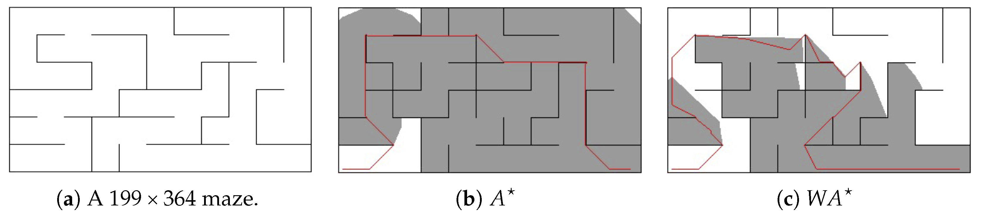
$A^{★}$ is optimal if the used heuristic function is admissible, i.e., never overestimates when predicting the distance to reach the goal [2]. Weighted$A^{★}$ ($W{A}^{★}$) [3] relaxes the admissibility rule and multiplies the heuristic function by a factor $ϵ>1$. While doing so might lead to finding sub-optimal paths, inflating the heuristic forces the search algorithm to prioritize exploring more promising paths rather than exploring every possible path to guarantee optimality. For example, Figure 1 compares the number of visited nodes in both $A^{★}$ and $W{A}^{★}$ (with $ϵ=3$) when trying to find the same path in an 8-neighbor grid map of a $199\times 364$ maze. Both algorithms use the octile-distance heuristic, which is a commonly-used admissible heuristic function that allows both straight and diagonal movements. As shown by Figure 1c, the greedy nature of $W{A}^{★}$ led it to prioritizing the exploration of the closer nodes to the goal, which resulted in finding a different, sup-optimal path. By contrast, $A^{★}$ slowly explores all similar nodes, i.e., nodes with the same cost, to guarantee optimality (as shown by Figure 1b).

Figure 1. Visited nodes (shown in dark grey) during optimal pathfinding using $A^{★}$ and sub-optimal pathfinding using weighted$A^{★}$ ($W{A}^{★}$) (with $ϵ=3.0$) for the path shown in red. Note that the source node is at the right-bottom and the goal node is the left-bottom of the map.

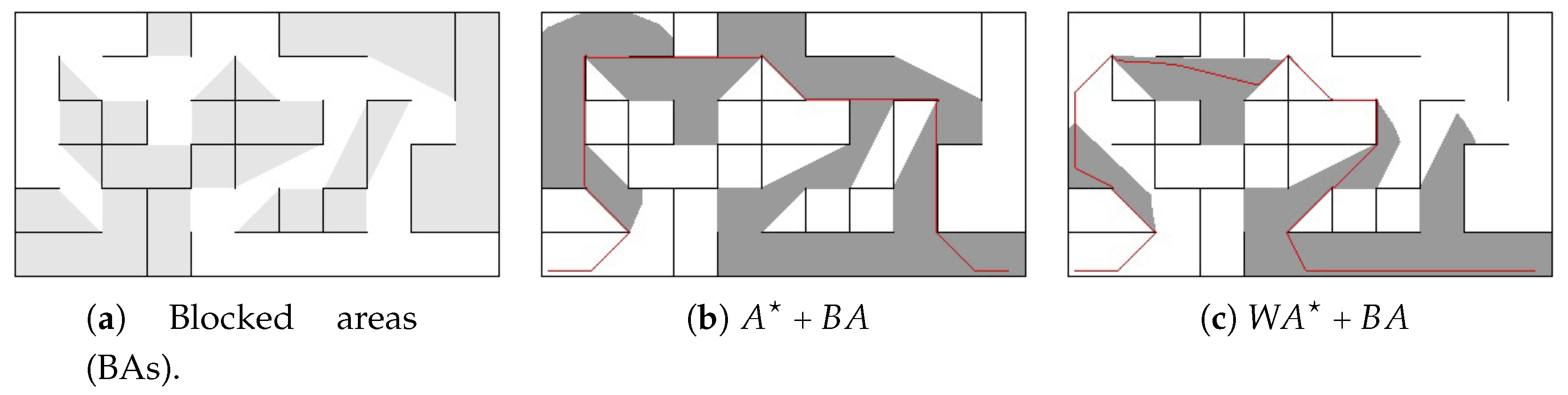
$W{A}^{★}$ is a simple yet effective extension of $A^{★}$ and is still in wide use to this day [4,5]. However, $W{A}^{★}$, as well as $A^{★}$, has no knowledge about the geometry of obstacles in a grid map, which could mislead the search into exploring paths with blocked ends. For example, Figure 2a shows twenty two polygon-shaped areas with blocked ends in the maze of Figure 1a. We refer to such shapes as blocked areas (BAs) because they are bound by obstacles from all directions, except for the one direction where the search may enter this area. This paper aims to make knowledge about blocked areas in a grid map available during pathfinding. By doing so, a search algorithm can avoid exploring useless paths inside blocked areas, which in turn reduces search time. For example, Figure 1 shows that both $A^{★}$ and $W{A}^{★}$ have wastefully explored most of the blocked areas identified in Figure 2a. By comparison, Figure 2b,c show the potential of using the blocked areas’ knowledge into guiding both search algorithms to avoid exploring blocked areas and thus significantly reducing the number of visited nodes while performing pathfinding.

Figure 2. The impact of using the blocked areas’ knowledge on reducing the number of visited nodes in optimal and sub-optimal pathfinding for the same path in Figure 1.

To make use of the blocked areas’ knowledge, we propose the following approach. First, a preprocessing algorithm investigates the geometry of obstacles in a grid map and identifies blocked areas. Next, information about blocked areas is stored in a memory-efficient balanced binary search tree, referred to as the BA-tree. During actual pathfinding, a search algorithm accesses the BA-tree to determine if a particular node is inside a blocked area. If so, then this node is not explored, i.e., eliminated from the search space.

An important property of our proposed method is that it does not depend on any specific heuristic function. Instead, it utilizes the geometry of obstacles to eliminate irrelevant parts to the search, i.e., in a sense, it reduces a map to a new (more concise) map that a heuristic search algorithm can investigate at a faster speed using its original heuristic function. Therefore, our method is orthogonal to the search algorithm itself, and hence can be combined with many heuristic search algorithms in the literature. As a proof of concept, in this paper, we present and evaluate our proposed method using $A^{★}$ and $W{A}^{★}$ search algorithms combined with the octile-distance heuristic. Another important property of our approach is that it preserves the optimality of a search algorithm. We present mathematical proofs of this claim in Section 4.

In addition, our approach has a small memory overhead because nodes in a grid map need not store any information about blocked areas, which would scale poorly for large maps. Instead, during pathfinding, a search algorithm retrieves this information from the BA-tree, where the memory requirements are bound by a small fraction of nodes in a grid map, as will be explained by Section 5.

While the concept of blocked areas can be generalized to any obstacle shape, in this paper, we consider maps where obstacles are represented as vertical and horizontal line-segments, which in turn form blocked areas that are polygons. Such cases are commonly found in maps of mazes, buildings and transportation maps.

We evaluate the impact of using the blocked areas’ knowledge for $A^{★}$ and $W{A}^{★}$ using a publicly available benchmark set that includes sixty maps of mazes and rooms [6]. Our evaluation shows that the search space (i.e., the number of visited nodes during pathfinding) of $A^{★}$ is reduced by 34%, on average, for both mazes and rooms. This results in a significant reduction in search time for both $A^{★}$ and $W{A}^{★}$. Specifically, in mazes, the execution times of both $A^{★}$ and $W{A}^{★}$ were reduced by 10–35% (the average is $28\%$). In rooms, the execution times of both $A^{★}$ and $W{A}^{★}$ were reduced by 5–$57\%$ (the average is $30\%$). Our evaluation also demonstrated that the memory overhead associated with storing blocked areas’ information in memory during preprocessing and the time associated with accessing this information during pathfinding are both small.

The remainder of this paper is organized as follows: Section 2 surveys related work. Section 3 provides background information about $A^{★}$ and $W{A}^{★}$ search algorithms. Section 4 presents the definition of blocked areas. Section 5 describes the proposed preprocessing algorithm for finding blocked areas in a grid map. Section 6 describes the proposed algorithms for constructing and accessing the BA-tree. Section 7 evaluates the impact of using the blocked areas’s knowledge in reducing execution time for both $A^{★}$ and $W{A}^{★}$. Section 8 concludes the paper.

2. Related Work

Several heuristic search algorithms in the literature, such as $A^{★}$ and $W{A}^{★}$, assume no prior knowledge about maps. However, in many grid-based pathfinding domains, maps have static nature, i.e., their territories remain mostly the same. Examples of such domains are video games and city maps. Therefore, preprocessing approaches where prior knowledge about grid maps are utilized for the purpose of speeding up pathfinding has attracted many researchers due to the amortized runtime overhead (preprocessing needs to be executed only once).

In general, the efficiency of preprocessing approaches for pathfinding depends on the following: (i) the type of knowledge collected; (ii) the runtime overhead of accessing this knowledge during actual pathfinding; and (iii) the memory overhead of storing this knowledge. Below, we survey previously proposed preprocessing methods and describe their difference to our work.

Some researchers proposed preprocessing approaches where optimal paths between all or some nodes are pre-calculated and stored in a database, which is looked up during actual pathfinding [7,8,9,10]. While pathfinding in these approaches is fast and optimal, in general (despite using compression techniques) memory requirements are huge because memory is proportional to the number of nodes in a map. By contrast, the memory requirement in our work is bounded by the number of blocked areas, which is, in practice, a small fraction compared to the total number of nodes in a grid map.

Other researchers suggested using preprocessing to create an abstraction layer (or multiple layers) for each group of nodes in the map with pre-calculated local paths. During actual pathfinding, a path is found first using the abstract map. This path is then refined in a subsequent step for the original map. The returned path is, however, not guaranteed to be optimal. Examples of such works are [11,12,13].

A related approach to the abstraction method is introduced by [14], where all shortest paths between all pairs of nodes are abstracted (instead of abstracting each group of nodes in a grid map). This is done using a preprocessing step that identifies all subgoals in a map. A subgoal is a sequence of nodes such that a path between any pair of nodes inside a subgoal is optimal only if it is a part of the optimal path to the next subgoal. During actual pathfinding, an optimal high-level path between subgoals is found first. This path is then refined to an optimal low-level path.

Compared to abstraction-based approaches, our approach does not require any additional refinement steps when performing pathfinding. In addition, it needs not store in memory any knowledge about pre-computed local distances between nodes.

A similar work to ours is the dead-end heuristic [15], which describes areas that are irrelevant to the current search. During the preprocessing phase, the map is decomposed into smaller areas and a high-level abstract graph with nodes representing those small areas is created. During actual pathfinding, the search is split into two phases. The first phase identifies all nodes in the high-level graph that are relevant to the shortest path (the other nodes are called the dead-end areas). The second phase performs actual pathfinding while avoiding dead areas. Due to using an abstract graph, dead-end heuristic requires an extra step during pathfinding; a step that is not needed in our work.

Another similar work to ours is [16], which uses preprocessing to identify swamps, a collection of nodes that can be skipped during optimal pathfinding. Conceptually, swamps and blocked areas have the same definition. In addition, similar to our work, swamps require no additional refinement steps during search time. However, unlike our work, each node in a map is required to store an identifier that tells which swamp this node belongs to so that, during pathfinding, search for nodes inside swamps is blocked. Our approach also blocks search inside the blocked areas, however, without requiring nodes to store blocked areas’ identifiers (which would be memory-inefficient in large maps). Instead, this information is retrieved from a memory-efficient binary search tree data structure during pathfinding.

Similar to $A^{★}$ and $W{A}^{★}$, there are also other heuristic search algorithms in the literature that assume no prior knowledge about maps, such as the Explicit Estimation Search [17] and Jump Point Search [18] algorithms. Our work is complementary to those algorithms, i.e., pre-computed knowledge about blocked areas can be combined with those algorithms to reduce search time. As a proof of concept, this paper evaluates the impact of blocked areas’ knowledge on reducing search time for the $A^{★}$ and $W{A}^{★}$ algorithms.

The Grid-Based Path Planning Competition (GPPC) [19] was introduced in 2012 to facilitate comparing different search algorithms using a standard set of maps, some of which were created artificially and others were taken from commercial video games [6]. We use sixty available maps of mazes and rooms from the same set to evaluate the proposed approach in this work. Details of the competing algorithms in the GCCP are summarized by [20].

A noticeable related field to our work is route planning in transportation networks, in which preprocessing techniques have been proposed to find the shortest paths in road networks [21]. Some of these techniques have also been used in the context of grid-based pathfinding. For example, in the GCCP’15 contest, a route planning approach based on the contraction hierarchies (CH) algorithm [22] achieved competitive performance. During a preprocessing phase, the CH algorithm uses a node contraction method to augment the shortest paths between each pair of nodes in a graph with shortcuts. During actual pathfinding, the search makes use of these shortcuts to reduce the execution time.

3. Background

In this paper, a grid map is represented as a 2D array of points (or nodes), where each node is identified by x and y coordinates. In addition, each node has a flag to indicate if it is either an obstacle or a non-obstacle node. For a given node n, $adjacent\left(n\right)$ is the set of non-obstacle nodes that are reachable from n via a single movement, which can be vertical, horizontal or diagonal. Consider node $m\in adjacent\left(n\right)$, the movement cost from n to m is represented by the function c(n,m):

$$c(n,m)=\left\{\begin{array}{cc}1.0,\hfill & n\mathrm{to}m\mathrm{movement}\mathrm{is}\mathrm{either}\mathrm{vertical}\mathrm{or}\mathrm{horizontal}\hfill \\ \sqrt{2.0},\hfill & n\mathrm{to}m\mathrm{movement}\mathrm{is}\mathrm{diagonal}\hfill \end{array}\right.$$

Algorithm 1 shows the pseudo code for the classical $A^{★}$ algorithm, which finds the shortest path between a source node s and a goal node g in a grid map G. $A^{★}$ is a best-first search algorithm that gradually expands nodes along the way from s to g while prioritizing exploring node with better heuristic scores. When expanding a node q, the algorithm defines the following four values: gscore(q), which is the distance from the source node s to q; hscore(q), which is the algorithm’s “guess" of the distance from q to the goal node g; fscore(q) = gscore(q) + hscore(q), which represents the priority of q in the search; and $parent$(q), which is a pointer to the parent of q in the path from s to g.

The algorithm maintains two lists: open and closed. When expanding a node, it is put in the open list. Nodes in the open list are then iteratively explored by their increasing order of fscore. A node that has been explored is removed from the open list and is put in the closed list so that it is not explored again. When the goal node is found, the search terminates and the path is constructed by recursively following the parent pointers from the goal node to the source node.

The optimality of $A^{★}$ is only guaranteed if the heuristic function is admissible, i.e., estimated distance by hscore(q) is always less than or equal to the actual distance from q to the goal node g [2]. One simple way of never overestimating hscore(q) is always assuming a straight line movement from q to g. An example of such a heuristic function is the octile-distance function, which is popularly used in 8-connected grid maps where horizontal, vertical and diagonal movements are allowed. Specifically, the octile-distance from node q to a goal node g is equal to the minimum number of diagonal steps, plus the minimum number of either vertical or horizontal steps needed to go from q to g. The octile-distance is given by the equation

$$h\mathrm{score}(q)=\sqrt{2.0}\times \mathrm{minimum}(\Delta x,\Delta y)+1.0\times (\Delta x+\Delta y-\mathrm{minimum}(\Delta x,\Delta y\left)\right)$$

where $\Delta x$ is the number of horizontal steps and $\Delta y$ is the number of vertical steps from q to g. Note that minimum($\Delta x$,$\Delta y$) represents the number of diagonal steps from q to g.

Algorithm 1$A^{★}$ pathfinding

Input:  Grid map G with a source node s and a goal node g Output:  The shortest path between s and g in G $open$ ⇐ $empty$ list $closed$ ⇐ $empty$ list add s into $open$ with gscore(s)$=0$, fscore(s) = hscore(s), $parent$(s)$=null$ while$open$ is not empty do    $n\Leftarrow$ get and remove node with minimum fscore from $open$    if $n=g$ then       return path from s to g    end if    add n into $closed$    for each node $q\in adjacent\left(n\right)$ and $q\notin closed$ do        gscore${}^{\prime }$ ⇐ gscore(n) + c(q,n)        if $q\notin open$ then           add q into $open$ with gscore(q) = gscore${}^{\prime }$, fscore(q) = gscore(q) + hscore(q), $parent$(q)$=n$        else if gscore${}^{\prime }$ < gscore(q) then           update q in $open$ with gscore(q) = gscore${}^{\prime }$, fscore(q) = gscore(q) + hscore(q), $parent$(q)$=n$       end if    end for end while return$failure$

$W{A}^{★}$ has the same pseudo code in Algorithm 1 with only one modification: it calculates fscore(q) = gscore(q) + $ϵ$ × hscore(q), $ϵ>1$. As previously explained, this simple yet elegant modification adds a stronger greedy nature of the search algorithm that leads it to finding a path more quickly, albeit being a sub-optimal path. It is proven that the cost of the sub-optimal path found by $W{A}^{★}$ is bounded by $ϵ$ × the cost of the optimal path [2].

The speed at which the $A^{★}$ algorithm, as well as the $W{A}^{★}$ algorithm, finds a path is affected by the quality of its heuristic function. For example, if the heuristic function computes an inaccurate estimate of the to-go-distance to the goal node, then the search algorithm will waste time exploring uninteresting nodes, i.e., nodes that are not pertaining to the shortest path. As previously mentioned, in many grid maps, a heuristic function may compute inaccurate distance estimates due to their unawareness of blocked ends created by the geometry of obstacles. To this end, this paper aims to identify areas in a grid map with blocked ends and make use of this knowledge to enable search algorithms to avoid wasting time exploring nodes in such areas.

4. Blocked Area Definition

For a given undirected 2D grid map, a blocked area (BA) is a connected subgraph of adjacent non-obstacle nodes that is bound by a continuous but non-enclosing chain of obstacle nodes. A blocked area’s entrance is the imaginary straight line that connects the two end points of the obstacles’ chain. Intuitively, any path that connects a node inside a blocked area with a node outside the blocked area passes by its entrance.

Given a blocked area A, we define $entrance$(A) to be the set of all nodes that lie on the imaginary straight line of A’s entrance. As a result that nodes in a grid map are discrete, the imaginary line may not cross the nodes themselves, and instead, cross the squares that are formed by the nodes. Therefore, a more precise definition of $entrance$(A) is the set of all nodes that lie on the corners of the intersecting squares with the entrance’s imaginary straight line. The remaining set of nodes inside the blocked area are defined as $internal$(A). Both of these sets are mutually exclusive, i.e., if node $n\in internal$(A), then $n\notin entrance$(A), and vice versa. We also define $external$(A) to be the set of all nodes n such that $n\notin$$internal$(A) and $n\notin$$entrance$(A).

Given the aforementioned definition of a blocked area, all nodes in $internal$(A) and $entrance$(A) must be non-obstacle nodes. Otherwise, A is not a blocked area. Furthermore, due to not having obstacles inside or along the entrance of a blocked area A, the following two properties hold:

Property 1 

There is always a path between a node $n_1\in entrance$(A) and a node $n_2\in internal$(A).

Property 2 

There is always a shortest path between two nodes $n_1$ and $n_2$ $\in entrance$(A) such that this path does not pass by any node $n\in internal$(A).

The main claim of this paper is that blocked areas can be ignored during pathfinding without affecting the correctness and the optimality of a heuristic search algorithm. In below, Lemma 1 proves the correctness claim by showing that there is always an alternative path to any path that passes by a blocked area in a grid map. Lemma 2 proves the optimality claim by showing that there is an alternative path that is also optimal.

Lemma 1.

Consider a blocked area A and a pair of nodes s and g that are outside A. If there is a path between s and g that passes by an internal node inside A, then there is also another path between s and g that does not pass by an internal node inside A.

Proof. 

Let $path$(s,g) denote a path between s and g, where s, g∈$external$(A). Additionally, let us assume this path passes by a node $n\in internal$(A). In order to prove Lemma 1, we need to show that there is another path, i.e., $\widehat{path}$(s,g), such that n ∉ $\widehat{path}$(s,g).

First, because n ∈ $path$(s,g), we can rewrite $path$(s,g) = $path$(s,n) + $path$(n,g). Next, because $n\in internal$(A), both $path$(s,n) and $path$(n,g) cross A’s entrance. Therefore, we can rewrite $path$(s,g) = $path$(s,x) + $path$(x,n) + $path$(n,y) + $path$(y,g), where nodes x and $y\in entrance$(A). Note that $path$(x,n) and $path$(n,y) exist (Property 1). Next, because x and $y\in entrance$(A), $path$(x,y) exists such that $n\notin$$path$(x,y) (Property 2). Therefore, we can construct a new path $\widehat{path}$(s,g) such that $\widehat{path}$(s,g) = $path$(s,x) + $path$(x,y) + $path$(y,g), where all nodes in $path$(s,x), $path$(x,y) and $path$(y,g) $\notin internal$(A). □

Lemma 2.

Consider a blocked area A and a pair of nodes s and g that are outside A. If there is an optimal path between s and g that passes by an internal node inside A, then there is also another optimal path between s and g that does not pass by an internal node inside A.

Proof. 

Let $path$(s,g) denote a path between s and g (s, g∈$external$(A)) such that it passes by a node $n\in internal$(A). Additionally, let $path$(s,g) be an optimal path with cost c. From Lemma 1, there is at least one path between s and g, denoted $\widehat{path}$(s,g), such that $n\notin$ $\widehat{path}$(s,g). Let $\widehat{c}$ be the cost of $\widehat{path}$(s,g). In order to prove Lemma 2, we need to show that $\widehat{c}$ = c.

As we showed earlier, we can write $path$(s,g) = $path$(s,x) + $path$(x,n) + $path$(n,y) + $path$(y,g) and $\widehat{path}$(s,g) = $path$(s,x) + $path$(x,y) + $path$(y,g), where nodes x and $y\in entrance$(A). Let $c_1$, $c_2$ and $c_3$ be the cost of $path$(x,n), $path$(n,y) and $path$(x,y), respectively. Thus, $c-\widehat{c}=c_1+c_2-c_3$. To show that $\widehat{c}$ = c, we need to show $c_1+c_2-c_3=0$.

First, because c is optimal, $c\le \widehat{c}$. Thus, $c_1+c_2-c_3\le 0$. Second, due to Property 2, $path$(x,y) is optimal, i.e., it has a less or equal length to $path$(x,n) + $path$(n,y). Therefore, $c_3\le c_1+c_2$, which leads to $c_3-(c_1+c_2)\le 0$. Combining both inequalities, the only possible solution is $c_1+c_2-c_3=0$. □

5. Blocked Area Detection

In this paper, we consider grid maps where obstacle nodes are adjacent to each other such that they form vertical or horizontal line-segments. In such grid maps, blocked areas have polygon shapes with internal non-obstacle nodes and a non-enclosing perimeter of obstacle nodes. The open side of the blocked area’s perimeter represents its entrance.

In a grid map, each line-segment obstacle is represented by two distinct nodes, i.e., $e_1$ = ($x_1$,$y_1$) and $e_2$ = ($x_2$,$y_2$), which are its end points. A horizontal line-segment obstacle has the same x-coordinate in both of its end points. A vertical line-segment obstacle has the same y-coordinate in both of its end points. We use the notation $e_1\to e_2$ to refer to a line-segment obstacle.

A vertical and a horizontal line-segment obstacles may intersect in a grid map. To identify such a scenario, we introduce a data structure called corner, which is represented by three distinct nodes v, t and h, where t is the intersection point, v is the end point of the vertical side and h is the end point of the horizontal side. We use the notation $v\to t\to h$ to refer to a corner. Note that when a horizontal and a vertical line-segment obstacle intersect, up to four corners with different geometrical shapes can be generated. For example, the intersection + has a single intersection point and four corners with the following shapes: ┌, └, ┐ and ┘.

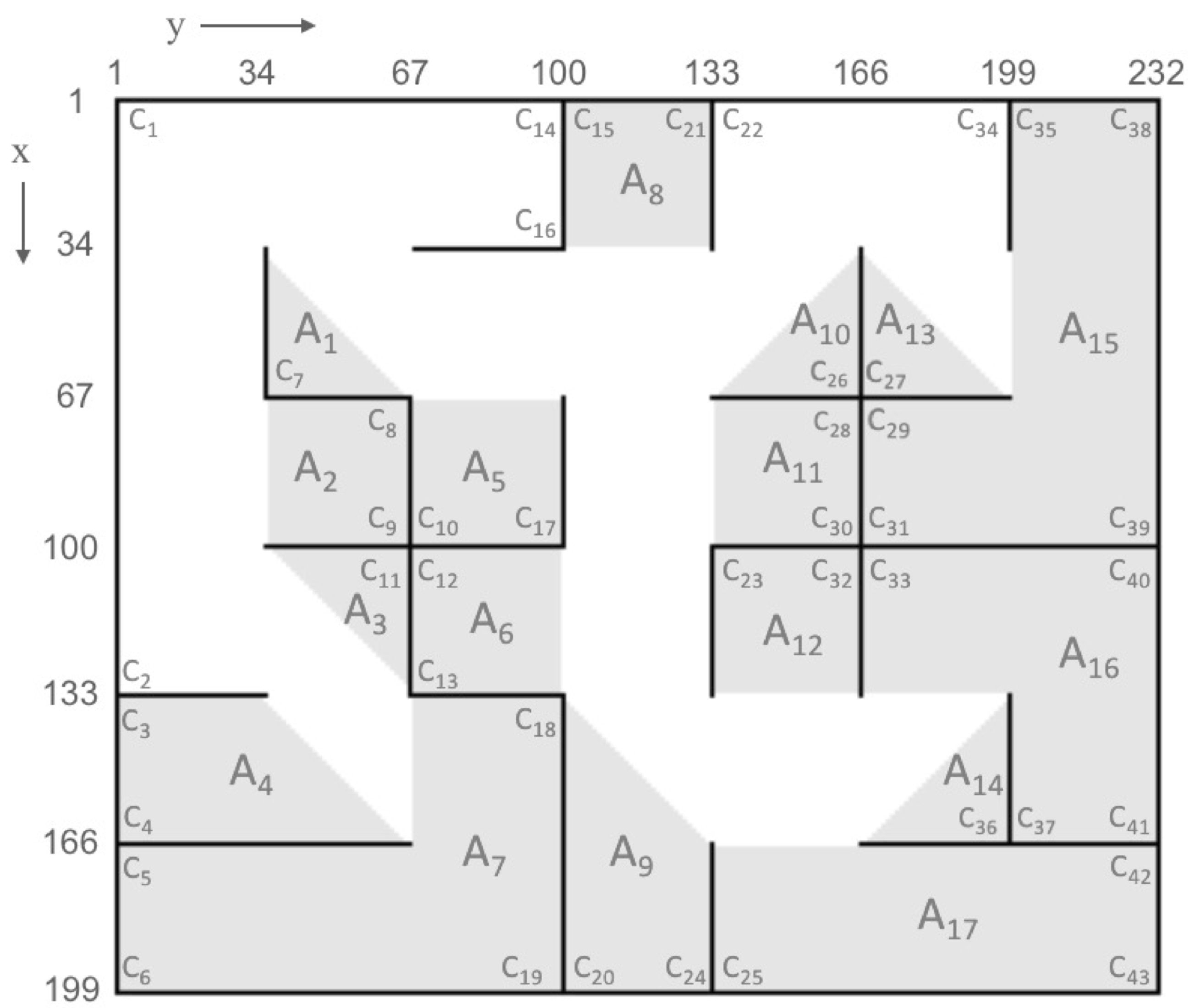
Figure 3 shows an example of a maze with 11 and 13 horizontal and vertical line-segment obstacles, respectively. Those obstacles intersect in 24 different intersection points such that 43 corners are generated. For example, the vertical line-segment (67,67)→(133,67) intersects with the horizontal line-segment (100,34)→(100,100). As a result, the four corners $C_9$, $C_{10}$, $C_{11}$ and $C_{12}$ are generated, where $C_9$ is represented by (67,67)→(100,67)→(100,34), $C_{10}$ is represented by (67,67)→(100,67)→(100,100), $C_{11}$ is represented by (133,67)→(100,67)→(100,34) and $C_{12}$ is represented by (133,67)→(100,67)→(100,100).

Figure 3. A 2D grid map of a $199\times 232$ maze with 11 horizontal and 13 vertical line-segment obstacles. The x-coordinates of the horizontal obstacles and the y-coordinates of the vertical obstacles are shown on the left and the upper sides of the map, respectively. In the map, there are 43 corners marked as $C_1$, $C_2$, …, $C_{43}$ and 17 blocked areas marked as $A_1$, $A_2$, …, $A_{17}$. The blocked areas in the map (excluding their entrances) are shown as shaded grey areas.

In a grid map, a polygon-shaped blocked area is formed when one or more corners are connected together such that a subset of non-obstacle nodes are bound within a continuous (but non-enclosing) chain of vertical and horizontal line-segment obstacles. For example, in Figure 3, blocked area $A_7$ is bound by the continuously connected corners (written in counterclockwise order): $C_5$, $C_6$, $C_{19}$ and $C_{18}$. Similarly, blocked area $A_{15}$ is bound by the continuously connected corners: $C_{29}$, $C_{31}$, $C_{39}$, $C_{38}$ and $C_{35}$. An interesting case is $A_1$, which is a triangular-shaped blocked area that was formed by the single corner $C_7$.

A polygon-shaped blocked area is represented by its perimeter joint points, which can be extracted from its corners. For example, consider blocked area $A_{17}$ in Figure 3, which is formed by the corners $C_{25}$, $C_{43}$ and $C_{42}$ (sorted in counterclockwise order). This blocked area is represented by the five points (166,133)→(199,133)→(199,232)→(166,232)→(166,166). The middle three points are the intersection points of $C_{25}$, $C_{43}$ and $C_{42}$, respectively. The first and the last points are the free points in $C_{25}$ and $C_{42}$. The entrance is represented by the straight line (166,166)→(166,133).

In general, a polygon-shaped blocked area with s corners (sorted in counterclockwise order): $C_1$, $C_2$, …, $C_s$ can be represented by $s+2$ joint points: $e_1$, $t_1$, $t_2$, …, $t_s$, $e_s$, where $t_i$ is the intersection point of corner $C_i$ and $e_1$ and $e_s$ are the free points of the two corners $C_1$ and $C_s$, respectively. The entrance is represented by the straight line between $e_1$ and $e_s$.

A simple and key observation is the following: a corner can only be in one unique blocked area. In other words, different blocked areas in a grid map have disjoin sets of connected corners. Therefore, to identify blocked areas in a grid map, we propose the following approach. First, identify all corners that result from the intersections between vertical and horizontal line-segment obstacles in a grid map. Then, identify each disjoint subset of corners that belong to the same blocked area. Finally, extract joint points from these disjoint sets to represent each blocked area.

Algorithm 2 presents the pseudo code for a preprocessing algorithm that performs the aforementioned approach. Firstly, in lines 1–2, Algorithm 2 uses the sweep line algorithm [23] to identify all intersection points between vertical and horizontal line-segments obstacles. The sweep line algorithm is a widely-used method for finding line-line intersections in Euclidean spaces due to its linearithmic performance [24]. Subsequently, Algorithm 2 extracts all corners from all intersections. Extracting corners from an intersection is straightforward (For brevity, pseudo codes of straightforward functions are not shown.).

Secondly, in lines 3–10, Algorithm 2 identifies which corners are connected. To do so, we propose the Partition and Sort method, which identifies all pairs of connected corners for every horizontal and vertical line-segment obstacle in a grid map. To explain, consider the horizontal line-segment obstacle (100,133)→(100,232), where the intersection points of the corners $C_{23}$, $C_{30}$, $C_{31}$, $C_{32}$, $C_{33}$, $C_{39}$ and $C_{40}$ are located. Our method first partitions the corners into two sublists: upward corners and downward corners. Upward corners are the corners with their vertical side located upward from the horizontal line-segment obstacle, which include corners $C_{30}$, $C_{31}$ and $C_{39}$. Downward corners are the corners with their vertical side located downward from the horizontal line-segment obstacle, which include $C_{23}$, $C_{32}$, $C_{33}$ and $C_{40}$. Next, our method sorts the corners in each sublist according to the y-coordinates of their vertical sides so that adjacent corners are next to each other. In the sorted order, each adjacent pair of corners with distinct intersection points are connected. For example, sorting the upward corners will give $C_{30}$, $C_{31}$ and $C_{39}$. The first adjacent pair ($C_{30}$, $C_{31}$) are not connected because they have the same intersection point, while the second adjacent pair ($C_{31}$, $C_{39}$) are connected due to having distinct intersection points. Similarly, sorting the downward corners will give $C_{23}$, $C_{32}$, $C_{33}$ and $C_{40}$, where only two adjacent pairs are connected: ($C_{23}$, $C_{32}$) and ($C_{33}$, $C_{40}$). Algorithm 3 presents the pseudo code for our proposed Partition and Sort method. Similar to horizontal line-segment obstacles, the Partition and Sort method is applied to vertical line-segment obstacles but while partitioning to left and right (instead of up and down) and sorting by x-coordinates (instead of sorting by y-coordinates).

Algorithm 2 Blocked Area Detection Algorithm

Input:  Grid map G with a set of vertical line-segment obstacles V and a set of horizontal line-segment obstacles H. The number of intersections is R and the number of corners is N. Output:  List of all blocked areas in G 1: $t_1$, $t_2$, …, $t_R$ ⇐ SweepLineAlgorithm(V, H) 2: $C_1$, $C_2$, …, $C_N$ ⇐ extractCorners($t_1$, $t_2$, …, $t_R$) 3: $UF\Leftarrow$ a union-find data structure with initially N disjoint corners: $C_1$, $C_2$, …, $C_N$ 4: for each line L in $V\cup H$ do 5:    $cornersublist$ ⇐ subset of corners with intersection points in L 6:    $connectedPairs$ ⇐ PartitionAndSort($cornersublist$,L) 7:    for each pair of corners $C_i$ and $C_j$ in $connectedPairs$ do 8:       $UF$.union( $C_i$, $C_j$ ) 9:     end for 10: end for 11: $BAlist\Leftarrow$ an initially empty list of blocked areas 12: for each disjoint set S in $UF$ do 13:    $C_1$, $C_2$, …, $C_s$ ⇐ get corners in S 14:    sort $C_1$, $C_2$, …, $C_s$ counterclockwise 15:    $e_1$, $t_1$, $t_2$, …, $t_s$, $e_s$ ⇐ extractJoints($C_1$, $C_2$, …, $C_s$) 16:    $A\Leftarrow$ createBlockedArea($e_1$, $t_1$, $t_2$, …, $t_s$, $e_s$) 17:    add A to $BAlist$ 18: end for 19: for each blocked area A in $BAlist$ do 20:    if $entrance$(A) has obstacle nodes or $internal$(A) has obstacle nodes then 21:        remove A from $BAlist$ 22:    end if 23: end for 24: return$BAlist$

The Partition and Sort method identifies connected corners in pairs. However, a blocked area can have multiple connected corners. To find all connected corners, we propose using a union-find data structure, which is a commonly-used data structure for keeping track of connected components in graphs (Sedgewick and Wayne, 2011). A union-find data structure starts by initially assuming all corners are disjoint and put into separate sets. Then, every time a pair of corners are found to be connected by the Partition and Sort method, union-find data structure unions their sets. By doing so for all pairs of connected corners in a grid map, the union-find data structure will have all connected corners put in the same set. Furthermore, all sets in the union-find data structure are disjoint.

Algorithm 3 Partition and Sort method

Input:  Set of l corners: $C_1$, $C_2$, …, $C_l$ with intersection points located on line-segment obstacle L. Output:  All pairs of connected corners on L 1: $connectedPairs$ ⇐ an initially empty list 2: ifL is horizontal then 3:    $upward$ ⇐ an initially empty list 4:    $downward$ ⇐ an initially empty list 5:    $x_L$ ⇐x-coordinate of L 6:    for each corner $C_i$ in $C_1$, $C_2$, …, $C_l$ do 7:       $x_i$ ⇐ x-coordinate of the vertical end point of $C_i$ 8:       if $x_i<x_L$ then 9:          add $C_i$ to $upward$ 10:     else 11:         add $C_i$ to $downward$ 12:       end if 13:    end for 14:    sort corners in $upward$ and $downward$ by the y-coordinate of their intersection points 15:    for each adjacent pairs of corners $C_i$ and $C_j$ in $upward$ and $dowward$ do 16:        if $C_i$ and $C_j$ have distinct intersection points then 17:            add ($C_i$,$C_j$) to $connectedPairs$ 18:        end if 19:    end for 20: else ifL is vertical then 21:    $left$ ⇐ an initially empty list 22:    $right$ ⇐ an initially empty list 23:    $y_L$ ⇐ y-coordinate of L 24:    for each corner $C_i$ in $C_1$, $C_2$, …, $C_l$ do 25:       $y_i$ ⇐ y-coordinate of the horizontal end point of $C_i$ 26:       if $y_i<y_L$ then 27:          add $C_i$ to $left$ 28:       else 29:          add $C_i$ to $right$ 30:       end if 31:    end for 32:    sort corners in $left$ and $right$ by the x-coordinate of their intersection points 33:    for each adjacent pairs of corners $C_i$ and $C_j$ in $left$ and $right$ do 34:       if $C_i$ and $C_j$ have distinct intersection points then 35:           add ($C_i$,$C_j$) to $connectedPairs$ 36:       end if 37:    end for 38: end if 39: return$connectedPairs$

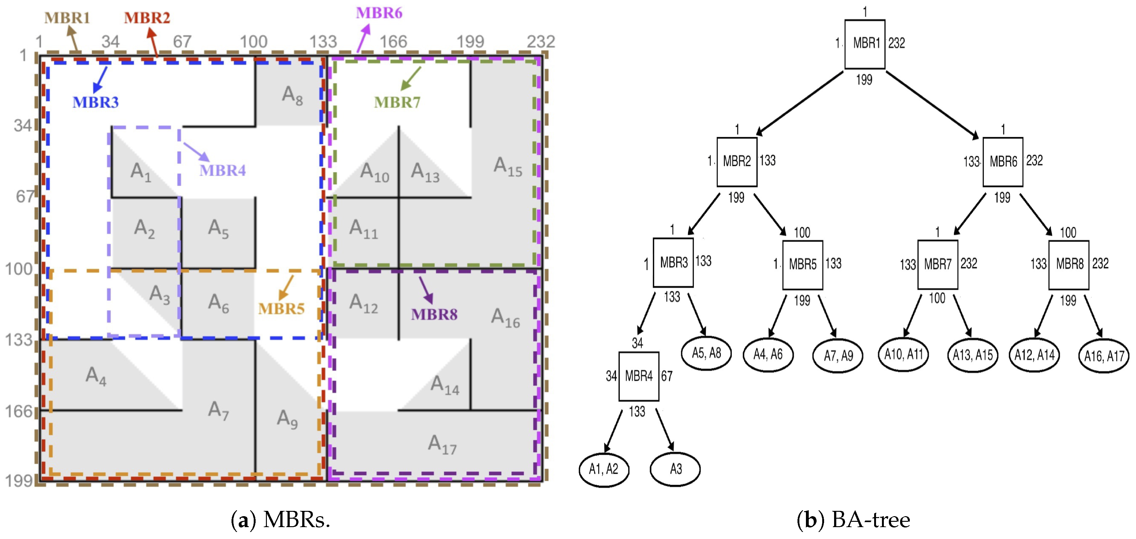
Thirdly, in lines 11–18, Algorithm 2 creates polygon-shaped blocked areas by extracting their perimeter’s joint points from every disjoint set of corners in the union-find data structure.

Finally, in lines 19–23, Algorithm 2 removes all blocked areas that do not satisfy our definition in Section 4, which stated that all internal and entrance nodes must be non-obstacle nodes. For example, in Figure 3, $C_{22}$ and $C_{34}$ form a blocked area. However, this blocked area is discarded because its entrance intersects with the vertical line-segment obstacle (34,166)→(133,166)), i.e., it has obstacle nodes in its entrance. Another example are corners $C_{16}$, $C_{14}$, $C_1$ and $C_2$, which form a blocked area that was discarded because it has internal obstacle nodes.

The detailed description of how Algorithm 2 determines which blocked areas have obstacles in their $entrance$ or $internal$ sets is not shown but can be explained as follows. As a result that a blocked area’s entrance is a straight line, the sweep line algorithm is used to determine if there is any horizontal or vertical line-segment obstacle that intersects with the entrance of a blocked area A. If so, A is discarded. Additionally, we modify the sweep line algorithm so that it can be used to identify all blocked areas with internal vertical or horizontal line-segment obstacles. Those blocked areas are also discarded.

Lemma 3.

The generated set of polygon-shaped blocked areas by Algorithm 2 satisfy the definition given in Section 4, i.e., each polygon-shaped blocked area is a connected subgraph of adjacent non-obstacle nodes that is bound by a continuous but non-enclosing chain of obstacle nodes.

Proof. 

As previously explained, in lines 1–18, Algorithm 2 identifies all non-enclosing polygon shapes of obstacles that represent blocked areas in a map. Then, in lines 19–23, Algorithm 2 determines which non-enclosing polygon shapes have obstacles in their $entrance$ or $internal$ sets and ensures that they are removed, i.e., not recognized as blocked area. Thus, Algorithm 2 guarantees that each polygon-shaped blocked area in the final output is a connected subgraph of adjacent non-obstacle nodes that are bound by a continuous but non-enclosing chain of vertical and horizontal line-segment obstacles (i.e., obstacle nodes). □

We now present a complexity analysis of Algorithm 2’s execution time. For convenience, let us assume, in a grid map, that $T_V$ is the number of vertical line-segment obstacles, $T_H$ is the number of horizontal line-segment obstacles, R is the number of intersections, N is the number of corners and P is the number of blocked areas. The following inequalities hold:

• $R\le T_V\times T_H$
  The maximum number of possible intersections occurs when every vertical line-segment obstacle intersects with every horizontal line-segment obstacle.
• $R\le N\le 4\times R$
  Each intersection generates anywhere between one to four corners.
• $P\le N$
  The maximum number of blocked areas occurs when each corner, alone, forms a triangular-shaped blocked area.

Table 1 describes an execution time complexity analysis for Algorithm 2. Authors in [24] have shown that, for a given Cartesian space with n line-segments and k intersections, the sweep line algorithm is bound by $n{log}_{2}n+k$. This explains the upper bounds shown for lines 1 and 19–23 in Table 1. In addition, note that we use the weighted union-find data structure (Sedgewick and Wayne, 2011), which guarantees that union operations are executed in logarithmic-time. Therefore, in lines 4–10, the most expensive operation inside the loop is the Partition and Sort method. Specifically, let us assume that the number of corners in $cornersublist$ is $N_l$, the Partition and Sort needs linear time (i.e., $N_l$) to partition the corners and linearithmic time (i.e., $N_l{log}_2{N}_l$) to sort the corners. Due to having a loop, the overall execution of the Partition and Sort method is bound by $N+N{log}_{2}N$. Finally, in lines 11-18, the most expensive operation in the loop is the sort operation in line 14. Hence, the overall loop’s execution is bound by $N{log}_{2}N$.

Table 1. Complexity analysis of Algorithm 2’s execution time.

Lines	Upper Bound Complexity	Explanation
1	($T_V+T_H$) ${log}_2(T_V+T_H)+R$	Sweep Line Algorithm
2	N	Extracting N corners from R intersections
3	N	Initializing union-find with N corners
4 – 10	$N+N{log}_{2}N$	The Partition and Sort method applied for a sub-list of corners inside a loop
11 – 18	$N{log}_{2}N$	Sorting a sub-list of corners inside a loop
19 – 23	($T_V+T_H+P$) ${log}_2(T_V+T_H+P)+P$	Sweep Line Algorithm

By taking into account the above three inequalities, the entire execution of Algorithm 2 is bound by ($T_V+T_H+P$) ${log}_2(T_V+T_H+P)$+N${log}_{2}N$. This shows that the preprocessing time of Algorithm 2 has an efficient linearithmic growth.

By the end of its execution, Algorithm 2 will identify all polygon-shaped blocked areas in a grid map. Each polygon-shaped blocked area is represented by its perimeter joint points, i.e., each blocked area is stored in memory using pointers that point to the nodes located at these joints. Assuming $J_i$ is the number of joints in blocked area $A_i$, the total number of extra pointers needed to store all blocked areas is ${\displaystyle J=\sum _{i=1}^P{J}_i}$. In practice, even for large maps, J represents a small fraction compared to the total number of nodes in a map. For example, in all of our benchmark set in Section 7, J is less than 5.4% of the total number of nodes in the map.

6. BA-Tree

As previously mentioned, our approach uses pre-computed knowledge about blocked areas in a map to prohibit a search algorithm from unnecessarily exploring nodes inside blocked areas. This is achieved using the BA-tree, a binary tree data structure that stores blocked areas’ information. During actual pathfinding, a search algorithm accesses the BA-tree to determine whether a particular node is inside a blocked area. If so, this node is discarded. In below, we first describe a preprocessing algorithm that constructs the BA-tree. Then, we describe an algorithm for accessing the BA-tree.

6.1. BA-Tree Construction

In computer science, spatial searching refers to the problem of locating objects in multi-dimensional spaces. R-tree data structures [25] have been extensively used for handling spatial searching in many contexts such as database applications and geographic information system applications [26]. The basic idea of R-tree data structures is to recursively subdivide a multi-dimensional space into subspaces such that nearby objects are grouped together into the same subspace. Those subspaces are then organized into a tree data structure, which in turn is used for servicing search queries. In this paper, we present the BA-tree, a variant of R-tree that is applied in the context of 2D grid-based pathfinding. Specifically, the BA-tree is a balanced binary search tree that is used for identifying which blocked area a given node belongs to in a 2D grid map.

For convenience, we first present the definition of the minimum bounding rectangle (or MBR) (The same terminology was used in the literature of R-tree data structures), which is the smallest rectangle that encapsulates a group of nearby blocked areas. Formally, we define MBR($A_1$, $A_2$, …, $A_m$) to be the smallest rectangle that bounds a group of m blocked areas: $A_1$, $A_2$, …, $A_m$. An MBR is represented by four coordinates: $x_{upper}$, the coordinate of the upper-most row; $x_{lower}$, the coordinate of the lower-most row; $y_{left}$, the coordinate of the left-most column; $y_{right}$, the coordinate of the right-most column. For example, in Figure 3, MBR($A_{10}$, $A_{11}$, $A_{13}$, $A_{15}$) is represented by $x_{upper}=1$, $x_{lower}=100$, $y_{left}=133$ and $y_{right}=232$.

Given a grid map with m blocked areas, the BA-tree is constructed as follows. Initially, an MBR that spans all m blocked areas is created. This MBR is then partitioned vertically into two MBRs such that each nearby $\frac{m}{2}$ blocked areas are put in the same MBR. Each MBR is then partitioned horizontally into two MBRs such that each nearby $\frac{m}{4}$ blocked areas are put in the same MBR. This is done recursively while alternating between vertical partitioning and horizontal partitioning. The recursive partitioning terminates when one or two blocked areas are reached. The resulting MBRs from the recursive partitioning are organized to form the following binary tree data structure:

• Internal nodes represent MBRs while leaf nodes represent blocked areas.
• At level 0 of the tree, there is only one node, the root node, which represents the MBR that encapsulates all m blocked areas.
• At level 1 of the tree, there are two nodes, which represent the two MBRs generated from applying vertical partitioning to the MBR of the node at level 0.
• At level 2 of the tree, there are four nodes, which represent the four MBRs generated from applying horizontal partitioning to the MBRs of the two nodes at level 1.
• In general, at level l of the tree, there are 2${}^l$ nodes, which are generated from partitioning the 2${}^{l-1}$ nodes at level $l-1$ of the tree. This partitioning is vertical if l is odd, while it is horizontal if l is even.

Algorithm 4 presents pseudo code for the vertical and horizontal partitioning functions that construct the BA-tree for a grid map. To simplify partitioning, both functions use sorting (line 11) to ensure that nearby blocked areas are adjacent to each other. Both functions recursively call each other (lines 12–13) to alternate the partitioning process. As an example, Figure 4 shows the BA-tree constructed by Algorithm 4 for the maze in Figure 3. Note that MBRs in different internal nodes may overlap. In below, we show few key properties of the BA-tree.

Figure 4. The BA-tree constructed by Algorithm 4 for the maze in Figure 3: (a) All generated minimum bounding rectangles (MBRs) are shown (different colors are used to help the reader distinguish each MBR). MBRs are numbered by the order of their creation by Algorithm 4; (b) The BA-tree is shown. Rectangle shapes are used for internal nodes to highlight the fact that they represent MBRs. In addition, each rectangle have four numbers shown on each one of its sides to show its $x_{upper}$, $x_{lower}$, $y_{left}$ and $y_{right}$ coordinates. Each leaf node may have only one or two blocked areas.

Lemma 4.

Assuming m is the number of blocked areas in a grid map, the height of the BA-tree is $\lceil {log}_{2}m\rceil -1$.

Proof. 

In a binary tree, the height is equal to the maximum level of a node in the BA-tree. Therefore, our goal is to show that all nodes in the BA-tree are located at levels $\le \lceil {log}_{2}m\rceil -1$.

Without loss of generality, let us first assume the simple case when m is a power of 2, i.e., $m=2^d$, where d is some integer. In this case, the levels of the BA-tree are: 0, 1, …, $d-1$, where $d-1$ is the last level because the recursive partitioning terminates when number of blocked areas is 2 (line 1 in Algorithm 4). Thus, the height of the tree is $d-1$ = ${log}_{2}m-1$.

In the general case, let h be the height of the BA-tree. Furthermore, let d be an integer such that $2^{d-1}<m\le 2^d$. First, $h\le d-1$ because $m\le 2^d$ and $d-1$ is the height of a tree with $2^d$ nodes (as shown by the simple case). Second, $h>d-2$ because $m>2^{d-1}$ and $d-2$ is the height of a tree with $2^{d-2}$ nodes. Combining both inequalities, we can write $d-2<h\le d-1$. As a result that h is an integer, the only possible solution is $h=d-1$. As a result that $d=\lceil {log}_{2}m\rceil$ (generated from applying the logarithm function to the inequality $2^{d-1}<m\le 2^d$), then $h=\lceil {log}_{2}m\rceil -1$. □

Algorithm 4 BA-tree Construction Functions

Input  Set of m blocked areas: $A_1$, $A_2$, …, $A_m$ Output  Set of tree nodes representing the BA-tree Function  divideVertically ($A_1$, $A_2$, …, $A_m$) 1: if$m\le 2$then 2:     e ⇐ new leaf node 3:     if $m=1$ then 4:         e.put($A_1$) 5:     else 6:         e.put($A_1$, $A_2$) 7:     end if 8: else 9:     e⇐ new internal node 10:   e.put($MBR$($A_1$, $A_2$, …, $A_m$)) 11:   sort $A_1$, $A_2$, …, $A_m$ by their $y_{right}$ coordinate 12:   e.left ⇐ divideHorizontally ($A_1$, $A_2$, …, $A_{\lceil \frac{m}{2}\rceil }$) 13:   e.right ⇐ divideHorizontally ($A_{\lceil \frac{m}{2}\rceil +1}$, $A_{\lceil \frac{m}{2}\rceil +2}$, …, $A_m$) 14: end if 15: returne Function  divideHorizontally ($A_1$, $A_2$, …, $A_m$) 1: if$m\le 2$then 2:      e ⇐ new leaf node 3:      if $m=1$ then 4:          e.put($A_1$) 5:      else 6:         e.put($A_1$, $A_2$) 7:      end if 8: else 9:      e ⇐ new internal node 10:    e.put($MBR$($A_1$, $A_2$, …, $A_m$)) 11:    sort $A_1$, $A_2$, …, $A_m$ by their $x_{lower}$ coordinate 12:    e.left ⇐ divideVertically ($A_1$, $A_2$, …, $A_{\lceil \frac{m}{2}\rceil }$) 13:    e.right ⇐ divideVertically ($A_{\lceil \frac{m}{2}\rceil +1}$, $A_{\lceil \frac{m}{2}\rceil +2}$, …, $A_m$) 14: end if 15: returne

Lemma 5.

The BA-tree is a balanced binary tree.

Proof. 

Let m be the number of blocked areas in a grid map and h be the height of the BA-tree. To show that the BA-tree is balanced, we need to show that each leaf node in the BA-tree is located at either level $h-1$ or level h.

Without loss of generality, let us first assume the simple case when m is a power of 2, i.e., $m=2^d$, where d is some integer. In this case, it is easy to prove that the BA-tree is balanced because Algorithm 4 always partitions an MBR of an internal node e such that the number of blocked areas in the left subtree of e is equal to the number of blocked areas in the right subtree of e (lines 12–13). Furthermore, in this case, all leaf nodes are located exactly at level $d-1$ (because m is a power of 2 and the recursive partitioning terminates when the number of blocked areas is 2).

In the general case, let d be an integer such that $2^{d-1}<m\le 2^d$. As a result of $m>2^{d-1}$, there are no leaf nodes that can be located at a level that is smaller than $d-2$ (as shown by the simple case). Furthermore, because $m\le 2^d$, the maximum level in the BA-tree is $d-1$ (Lemma 4). Thus, all leaf nodes can only be located at levels $d-2$ and $d-1$. As a result of $h=d-1$ (Lemma 4), we can also infer that all leaf nodes are located at levels $h-1$ and h. □

Lemma 6.

Assuming m is the number of blocked areas in a grid map, the number of nodes in the BA-tree is bound by $2\times m-1$.

Proof. 

As a result that the number of nodes in level i is at most $2^i$, the maximum number of nodes in the BA-tree is bound by ${\displaystyle \sum _{i=0}^{\lceil {log}_{2}m\rceil -1}{2}^i}$. This is a geometric series that is equal to $2^{\lceil {log}_{2}m\rceil }-1$. $\lceil {log}_{2}m\rceil <{log}_{2}m+1$, $2^{\lceil {log}_{2}m\rceil }<2^{{log}_{2}m+1}=2\times m$. Thus, $2^{\lceil {log}_{2}m\rceil }-1<2\times m-1$. □

Corollary 1.

Assuming m is the number of blocked areas in a grid map, the number of internal nodes in the BA-tree is bound by $m-1$ and the number of leaf nodes is bound by m.

6.2. BA-Tree Analysis

We now present a complexity analysis of the execution time of Algorithm 4. Without loss of generality, let us assume the number of blocked areas m is a power of 2 and the height of the BA-tree is ${log}_{2}m$. In Algorithm 4, it is quite straightforward to observe that the sort operation in line 11 is the longest operation, i.e., execution time is bound by sorting time (which has the upper bound complexity of $n{log}_{2}n$, where n is the number of integers). At each level j in the BA-tree, there are $2^j$ nodes, i.e., subproblems. Each subproblem’s execution time is bound by sorting $\frac{m}{2^j}$ blocked areas. Therefore, the amount of work done by all nodes in level j is $2^j\times \frac{m}{2^j}{log}_2\frac{m}{2^j}=m{log}_2\frac{m}{2^j}\le m{log}_{2}m$. As a result that the height of the tree is ${log}_{2}m-1$ (Lemma 4), the amount of work done to construct all levels in the BA-tree is bound by $m{log}_2^{2}m$. In general, the execution time is bound by $m{\lceil {log}_{2}m\rceil }^2$.

We now present a memory consumption analysis for the BA-tree. As shown by Corollary 1, the number of internal nodes is bound by $m-1$, where m is the number of blocked areas. Each internal node stores four integers (the coordinates of its MBR) and two pointers ($left$ and $right$). Assuming pointers and integers require the same amount of memory, all internal nodes need to store no more than 6 × ($m-1$) integers. In other words, the needed memory for internal nodes in the BA-tree is bound by the number of blocked areas in a grid map. On the other hand, leaf nodes store the blocked areas: $A_1$, $A_2$, …, $A_m$. As previously mentioned in Section 5, the amount of memory needed to store blocked area’s information, denoted by J, is bound by the total number of joint points in blocked areas, which is, in practice, equal to a small fraction of the number of nodes in a grid map.

6.3. BA-Tree Access

Algorithm 5 presents pseudo code for a recursive search function that identifies which blocked area A in the BA-tree contains a particular node q in a grid map. Starting from the root node, the search function searches all the nodes in the BA-tree in a depth-first fashion, however, with a key optimization: when visiting an internal node e, if $q\notin$ MBR(e), then the search for the descendent nodes of e is terminated (lines 9–11). This is because, if $q\notin$ MBR(e), it is predetermined that $e\notin$ any of the descendent blocked areas of e. In the case $q\in$ MBR(e), the function continues the search in the left path of e (line 12). If a blocked area was not found in the left path (line 13), the function then searches the right path of e (line 14). Determining whether $q\in$ MBR(e) or not is straightforward: $q\in$ MBR(e) if and only if $x_{upper}\le q.x\le x_{lower}$ and $y_{left}\le q.y\le y_{right}$. In the case e is a leaf node (lines 1–8), the search function simply checks if q is contained by any of the blocked areas in e and terminates the search if such blocked area is found. Note that the maximum number of blocked areas in a leaf node is two. To determine if a polygon-shaped blocked area A contains a node q, we use the winding number algorithm [27], a widely-used method in computational geometry for determining if a point is inside a polygon. Figure 5 shows examples on two search queries for the BA-tree in Figure 4.

Algorithm 5 BA-tree Access Function

Input  Query node q in a grid map and node e in the BA-tree Output  Blocked area A to which q belongs to, or null if no such blocked area exists. Function  searchBAtree (q, e) 1: ife is a leaf then 2:     for each blocked area A in e do 3:       if $e\in$ internal(A) then 4:          return A 5:       end if 6:    end for 7:    return $null$ 8: end if 9: if$q\notin$$MBR$(e) then 10:    return null 11: end if 12: A ⇐ searchBAtree (q, e.left) 13: ifA = null then 14:     A⇐ searchBAtree (q, e.right) 15: end if 16: returnA

Figure 5. Two search examples using the BA-tree in Figure 4. Searched nodes are shown in grey.

The worst-case scenario in Algorithm 5 occurs when a search function visits all the nodes in the BA-tree, which is bound by $2\times m-1$ (Lemma 6), where m is the number of blocked areas. However, this is rarely needed because, in real maps, blocked areas are often scattered such that they are isolated from each other. Thus, in the common case, the search function only needs to check a subset of paths in the BA-tree. As a result that the height of the BA-tree is $\lceil {log}_{2}m\rceil -1$ (Lemma 4), the average-case execution time of Algorithm 5 is $\tau \times \lceil {log}_{2}m\rceil$, where $\tau$ is some constant.

6.4. BA-Tree Alternatives

We now describe two alternative schemes to store blocked areas’ knowledge and discuss their differences to the BA-tree. The first alternative scheme is to assign a unique numeric ID to each blocked area, and then use an extra grid, in which each node stores the ID of the corresponding blocked area, or an invalid ID if it is outside all blocked areas. Such a scheme would require O(1) access time and O(n) space, where n is the total number of nodes in a grid map. By contrast, the BA-tree is more memory-efficient because it stores information about only joint points, which represents a small fraction of the total number of nodes in a gird map. Furthermore, the BA-tree has a low access time overhead, as discussed earlier.

Another scheme is to use trapezoidal decomposition [28], i.e., divide blocked areas into a set of trapezoids such that each trapezoid is the portion of the sweep line between two adjacent corners. Trapezoids are neighbors if they are neighbors along the sweep line or if one appears when the other disappears at a sweep event. The number of trapezoids is bound by 3 × n, where n is the total number of line-segment obstacles in a grid map [28]. Identifying which trapezoid contains a particular node is a grid map is O(1). More specifically, the first node requires O(n) due to performing linear search. Afterward, identifying adjacent nodes requires constant time because they are found in adjacent trapezoids. The trapezoidal decomposition scheme provides better access time guarantees than the BA-tree. However, it requires more memory to store the trapezoids’ information.

7. Experimental Results

We evaluate the performance by showing the reduction in execution time for both $A^{★}$ and $W{A}^{★}$ algorithms after combining the knowledge of blocked areas in their search. We perform pathfinding for sixty maps of mazes and rooms taken from the public pathfinding benchmarks library [6]. The modified algorithms are denoted by $A^{★}+BA$ and $W{A}^{★}+BA$. All four search algorithms: $A^{★}$, $W{A}^{★}$, $A^{★}+BA$ and $W{A}^{★}+BA$ are implemented and compiled using Java SE 8 and all experiments were executed on a Red Hat Enterprise Linux 6 machine with a 2.2 GHz Intel Xeon-E5 processor and a 64 GB DDR3 memory with a speed of 1333 MHz.

Below, we describe, in detail, the implementation of the modified search algorithms and the tested benchmark set. Then, we present the evaluation results.

7.1. Search Implementation

Algorithm 6 shows the pseudo code for the implementation of $A^{★}+BA$ algorithm. Compared to the standard implementation of $A^{★}$ (shown in Algorithm 1), Algorithm 6 has two modifications. First, before adding node q into the $openlist$, the algorithm accesses the BA-tree (in line 14) using the search function presented in Algorithm 5 to determine the blocked area A where q is located. Second, in line 15–17, the algorithm inserts q into the $openlist$ (i.e., included in the search) only if one of the following three conditions are satisfied:

• q is not inside a blocked area.
• q is inside a blocked area; however, this blocked area also contains the goal node g. This condition ensures that the search never ignores a blocked area where the goal node is located.
• q is inside a blocked area; however, this blocked area also contains the parent node of q. This condition is needed in the case that the source node s happens to be inside a blocked area. If so, this blocked area is included in the search.

The aforementioned conditions are checked in the order shown, i.e., condition 2 is only checked if condition 1 is not satisfied and condition 3 is only checked if both conditions 1 and 2 are not satisfied. If none of the three conditions is satisfied, then q is not inserted into the $open$ list and therefore discarded from the search space. $W{A}^{★}$ and $W{A}^{★}+BA$ have the same implementations as $A^{★}$ and $A^{★}+BA$, respectively, except that they calculate fscore(q) = gscore(q) + $ϵ$ × hscore(q), where $ϵ>1$ is a real number that controls the inflation of the heuristic function hscore(q). In this paper, we set $ϵ=3.0$.

Algorithm 6$A^{★}+BA$ pathfinding

Input:  Grid map G with a source node s and a goal node g Output:  The shortest path between s and g in G 1: $open$ ⇐ $empty$ list 2: $closed$ ⇐ $empty$ list 3: $BAroot$ ⇐ the root node of the $BA$-tree 4: add s into $open$ with gscore(s)$=0$, fscore(s) = hscore(s), $parent$(s)$=null$ 5: while$open$ is not empty do 6:    $n\Leftarrow$ get and remove node with minimum fscore from $open$ 7:    if $n=g$ then 8:        return path from s to g 9:    end if 10:  add n into $closed$ 11:  for each node $q\in adjacent\left(n\right)$ and $q\notin closed$ do 12:      gscore${}^{\prime }$ ⇐ gscore(n) + c(q,n) 13:      if $q\notin open$ then 14:        A ⇐ searchBAtree (q, $BAroot$) 15:        if $A=null$ or $g\in A$ or $A=$ searchBAtree ($parent$(q), $BAroot$) then 16:          add q into $open$ with gscore(q) = gscore${}^{\prime }$, fscore(q) = gscore(q) + hscore(q), $parent$(q)$=n$ 17:        end if 18:     else if gscore${}^{\prime }$ < gscore(q) then 19:         update q in $open$ with gscore(q) = gscore${}^{\prime }$, fscore(q) = gscore(q) + hscore(q), $parent$(q)$=n$ 20:      end if 21:    end for 22: end while 23: return$failure$

An important note is that a tie may occur when extracting the node with the minimum f-score in the open list, i.e., there might be multiple nodes that have the same minimum f-score (line 6). In such a case, ties are broken in favor of the node with the largest g-score. Such tie-breaking strategy is common in the literature [29,30]. We use this strategy in the implementation of all four tested algorithms.

In all four algorithms, the $open$ list is implemented using a binary min heap data structure, while the closed list is implemented using a hash table data structure that uses chaining to resolve collisions.

7.2. Benchmark Set

Thirty grid maps of mazes and thirty grid maps of rooms were selected form the public pathfinding benchmarks library to evaluate performance in this paper. A maze’s map consists of corridors with fixed sizes that are randomly scattered. A room’s map consists of squares with fixed sizes that are uniformly distributed with randomly generated doors between every two adjacent rooms (squares). All sixty maps of mazes and rooms have 512 × 512 resolution, i.e., the number of nodes in each row and in each column is 512.

The thirty mazes are divided into three types, each of which has ten maps, which are: maze-8, maze-16 and maze-32, where 8, 16 and 32 are the sizes of the corridors in each type, respectively. Similarly, the thirty rooms are divided into three types, each of which has ten maps, which are: room-8, room-16 and room-32, where 8, 16 and 32 are the sizes of the squares in each type, respectively. The pathfinding benchmarks library also provides, for each grid map, hundreds of test cases with randomly generated source and goal points (called scenarios) for performing pathfinding. We use all of these scenarios in our evaluation (however, we discard invalid scenarios where either the source or the goal node is an obstacle).

Table 2 summarizes the evaluated benchmarks set. In all sixty maps, obstacles are represented as vertical and horizontal line-segments. Therefore, in Table 2, we also include information about the number of horizontal and vertical line-segment obstacles, as well as the number of intersections and corners in every map. All of these measurements are relevant to the blocked area detection algorithm presented in Section 5.

Table 2. The benchmark set used for performance evaluation in this paper. S is the number of scenarios available from the pathfinding benchmarks library. B% is the percentage of obstacle nodes in the map. H is the number of horizontal line-segment obstacles. V is the number of vertical line-segment obstacles. R is the number of intersections between horizontal and vertical line-segment obstacles. N is the number of corners generated from these intersections.

Map	S	B%	H	V	R	N	Map	S	B%	H	V	R	N
maze-8-0	5433	11%	817	804	1586	2315	room-8-0	1830	21%	3318	3332	3967	12,560
maze-8-1	8516	11%	837	779	1587	2334	room-8-1	1805	21%	3346	3340	3960	12,516
maze-8-2	9148	11%	818	803	1591	2370	room-8-2	1785	21%	3301	3314	3963	12,532
maze-8-3	9282	11%	847	789	1607	2369	room-8-3	1786	21%	3280	3329	3962	12,539
maze-8-4	10,796	11%	808	780	1553	2323	room-8-4	1840	21%	3344	3269	3956	12,555
maze-8-5	9304	11%	793	795	1552	2286	room-8-5	1800	21%	3341	3306	3963	12,564
maze-8-6	7087	11%	838	814	1619	2408	room-8-6	1811	21%	3309	3345	3951	12,562
maze-8-7	9360	11%	817	788	1575	2368	room-8-7	1857	21%	3312	3385	3972	12,528
maze-8-8	6667	11%	824	829	1621	2368	room-8-8	1838	21%	3329	3300	3961	12,519
maze-8-9	7486	11%	829	796	1592	2341	room-8-9	1787	21%	3312	3293	3964	12,588
maze-16-0	8412	6%	245	232	463	678	room-16-0	1833	12%	872	881	1015	3510
maze-16-1	7394	6%	248	237	468	689	room-16-1	1854	12%	867	876	1014	3527
maze-16-2	6231	6%	240	224	442	664	room-16-2	1898	12%	900	898	1012	3499
maze-16-3	8827	6%	252	229	465	680	room-16-3	1896	12%	891	897	1014	3507
maze-16-4	8195	6%	243	228	458	688	room-16-4	1852	12%	879	866	1016	3518
maze-16-5	6373	6%	242	228	456	677	room-16-5	1861	12%	905	901	1013	3500
maze-16-6	8723	6%	260	237	482	697	room-16-6	1866	12%	878	884	1017	3509
maze-16-7	7965	6%	241	229	453	678	room-16-7	1875	12%	894	887	1012	3508
maze-16-8	10,494	6%	241	235	461	672	room-16-8	1896	12%	906	870	1010	3503
maze-16-9	6723	6%	231	246	463	682	room-16-9	1821	12%	1005	954	1011	3489
maze-32-0	5603	3%	70	62	122	173	room-32-0	1844	8%	391	341	256	915
maze-32-1	4787	3%	65	53	110	165	room-32-1	1893	6%	248	252	256	929
maze-32-2	6938	3%	66	61	118	177	room-32-2	2015	6%	220	214	255	931
maze-32-3	7282	3%	65	57	113	176	room-32-3	1928	7%	313	313	256	922
maze-32-4	5227	3%	65	60	117	167	room-32-4	1665	10%	365	418	248	897
maze-32-5	5744	3%	67	65	121	177	room-32-5	1844	7%	285	277	254	929
maze-32-6	5519	3%	71	66	129	181	room-32-6	1896	6%	257	244	256	927
maze-32-7	4533	3%	63	59	114	164	room-32-7	1888	7%	311	311	255	923
maze-32-8	6098	3%	65	61	117	174	room-32-8	1959	6%	225	222	256	933
maze-32-9	7243	3%	57	54	104	154	room-32-9	2005	6%	247	255	256	929

7.3. Preprocessing Evaluation

Prior to performing pathfinding, in all sixty maps, a preprocessing step is executed to identify all blocked areas (using Algorithm 2), and then construct the BA-tree (using Algorithm 4). In some maps, some of the identified triangular-shaped blocked areas are small, i.e., they have one side with short length. As an optimization, such blocked areas were discarded because they are not useful during actual pathfinding. In all maps, preprocessing time was less than 300 milliseconds.

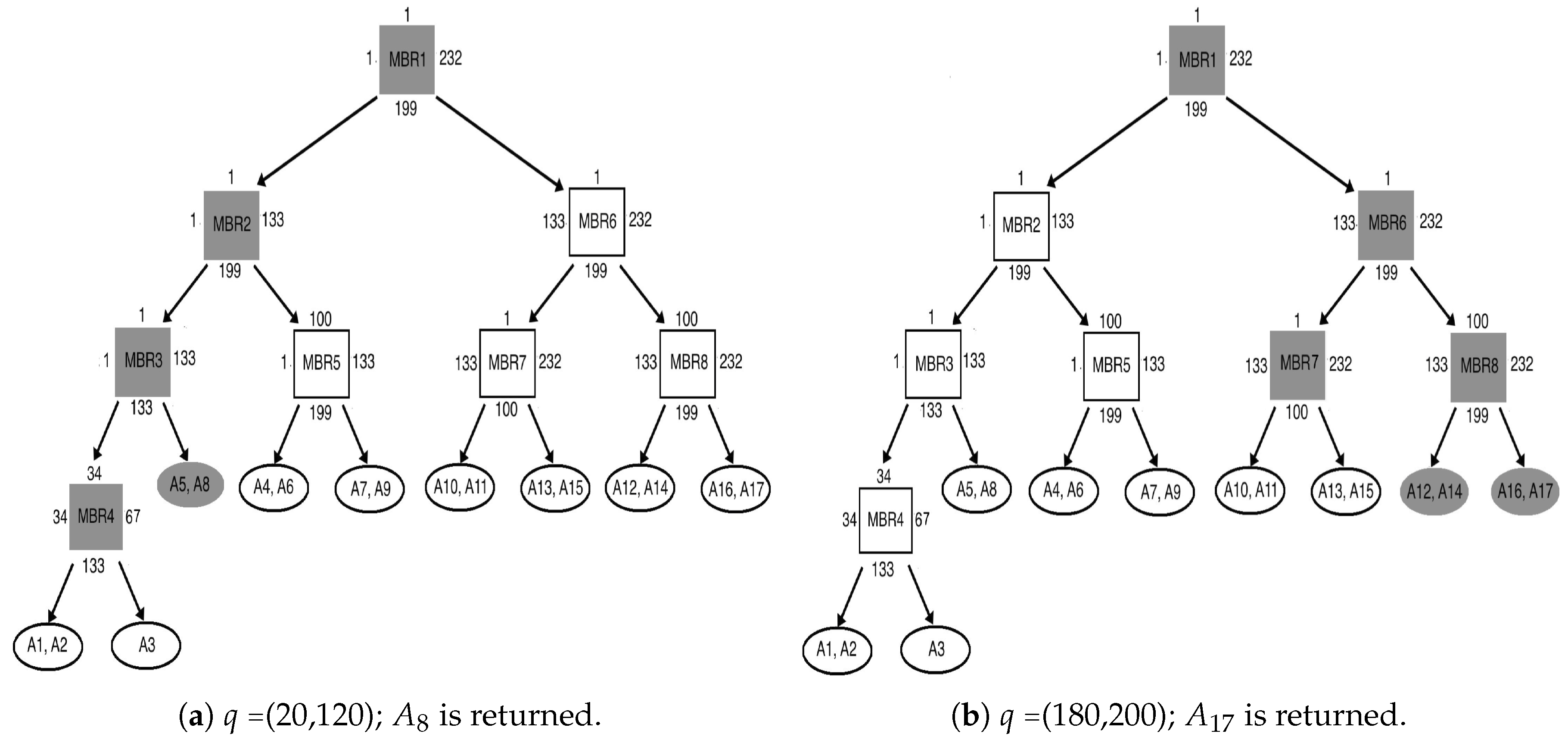
Table 3 presents an evaluation of the preprocessing step by showing the following measurements: (i) the number of blocked areas ($BA$); (ii) the percentage of nodes covered by those blocked areas (insideBA%); (iii) the percentage of nodes stored in memory due to blocked areas (joints%); (iv) the size of the BA-tree, i.e., the total number of tree nodes used to construct the BA-tree ($BASize$); and (v) the worst-case number of searched nodes when accessing the BA-tree ($Search$).

Table 3. Preprocessing evaluation for all sixty benchmarks in Table 2. $BA$ is the number of blocked areas. $insideBA\%$ is the percentage of nodes covered by blocked areas. $joints\%$ is the percentage of all nodes stored in blocked areas. $BASize$ is the total number of nodes in the BA-tree. $Search$ is the worst-case number of searched nodes when accessing the BA-tree using Algorithm 5.

Map	BA	insideBA%	joints%	BASize	Search	Map	BA	insideBA%	joints%	BASize	Search
maze-8-0	872	35.2%	1.3%	1023	45	room-8-0	3932	25.2%	5.4%	4095	63
maze-8-1	896	35.4%	1.3%	1023	51	room-8-1	3889	24.6%	5.3%	4095	61
maze-8-2	923	35.6%	1.3%	1023	51	room-8-2	3881	24.3%	5.3%	4095	61
maze-8-3	889	34.3%	1.3%	1023	49	room-8-3	3906	25.0%	5.3%	4095	59
maze-8-4	902	35.8%	1.3%	1023	47	room-8-4	3833	24.6%	5.2%	4095	57
maze-8-5	828	33.2%	1.2%	1023	55	room-8-5	3931	25.5%	5.4%	4095	59
maze-8-6	960	35.7%	1.3%	1023	53	room-8-6	3862	25.0%	5.3%	4095	55
maze-8-7	897	36.8%	1.3%	1023	49	room-8-7	3847	24.9%	5.3%	4095	57
maze-8-8	933	35.6%	1.3%	1023	53	room-8-8	3870	24.0%	5.3%	4095	59
maze-8-9	903	35.3%	1.3%	1023	51	room-8-9	3846	25.3%	5.3%	4095	71
maze-16-0	256	37.5%	0.4%	255	41	room-16-0	2007	40.4%	2.5%	2047	59
maze-16-1	261	37.0%	0.4%	265	41	room-16-1	1954	42.8%	2.5%	2047	61
maze-16-2	262	39.3%	0.4%	267	41	room-16-2	1967	40.2%	2.5%	2047	55
maze-16-3	254	38.9%	0.4%	255	37	room-16-3	1952	40.5%	2.5%	2047	53
maze-16-4	249	33.9%	0.4%	255	39	room-16-4	1968	42.2%	2.5%	2047	51
maze-16-5	230	34.6%	0.3%	255	37	room-16-5	1961	40.8%	2.5%	2047	61
maze-16-6	280	38.1%	0.4%	303	37	room-16-6	1955	41.7%	2.5%	2047	53
maze-16-7	253	37.3%	0.4%	255	37	room-16-7	1991	40.3%	2.5%	2047	53
maze-16-8	252	35.8%	0.4%	255	45	room-16-8	1913	41.5%	2.5%	2047	51
maze-16-9	248	38.3%	0.4%	255	37	room-16-9	1975	40.4%	2.5%	2047	57
maze-32-0	72	37.5%	0.1%	79	33	room-32-0	642	49.0%	0.8%	771	47
maze-32-1	65	40.7%	0.1%	65	29	room-32-1	625	51.2%	0.8%	737	45
maze-32-2	70	39.0%	0.1%	75	25	room-32-2	624	52.2%	0.8%	735	43
maze-32-3	68	32.3%	0.1%	71	31	room-32-3	637	51.1%	0.8%	761	47
maze-32-4	63	34.3%	0.1%	63	25	room-32-4	618	52.4%	0.8%	723	51
maze-32-5	74	34.0%	0.1%	83	27	room-32-5	638	51.5%	0.8%	763	43
maze-32-6	85	44.7%	0.1%	105	33	room-32-6	631	51.9%	0.8%	749	45
maze-32-7	68	38.4%	0.1%	71	23	room-32-7	629	52.8%	0.8%	745	47
maze-32-8	69	45.0%	0.1%	73	25	room-32-8	632	50.7%	0.8%	751	45
maze-32-9	56	36.1%	0.1%	63	31	room-32-9	628	52.0%	0.8%	743	47

In a grid map, the percentage of nodes covered by blocked areas represents an upper bound on the number of nodes that can be eliminated during pathfinding. On average, the percentages of covered nodes in maze-8, maze-16 and maze-32 are $35\%$, $37\%$ and $38\%$, respectively. On average, the percentages of covered nodes in room-8, room-16 and room-32 are $25\%$, $41\%$ and $52\%$, respectively.

As was previously mentioned in Section 5, blocked areas are stored in memory using pointers that point to nodes located at the joints of blocked areas. Table 3 shows that, in the worst-case, the total number of joints in blocked areas is less than $1.3\%$ of the total number of nodes in mazes and is less than $5.4\%$ in rooms. This demonstrates the memory efficiency of our approach.

While accessing the BA-tree is not part of preprocessing, in Table 3, we also measure the worst-case scenario of accessing the BA-tree. Specifically, we use the search function in Algorithm 5 to access the BA-tree using every node in a grid map as a search query, and then we report in Table 3 the worst-case number of how many nodes in the BA-tree were searched. In all sixty grid maps, the worst-case search needed was no more than $6\times {log}_{2}n$ nodes in the BA-tree, where n is the total number of nodes in the BA-tree. This shows that, in practice, the access time of the BA-tree is logarithmic.

7.4. Pathfinding Evaluation

We demonstrate the impact of the blocked areas’ knowledge in pathfinding using two comparisons: (i) $A^{★}+BA$ versus $A^{★}$; and (ii) $W{A}^{★}+BA$ versus $W{A}^{★}$. We do so by computing the relative execution time, which is a intuitive measurement of the reduction in execution time. For example, let us assume that the execution time of $A^{★}$ when performing pathfinding for a particular map is 500 milliseconds, while the execution time for $A^{★}+BA$ when performing the same pathfinding is 300 milliseconds. In this case, the relative execution time is $300/500=0.6$, which demonstrates that the execution time of $A^{★}$ was reduced by $40\%$ when using the blocked areas’ knowledge in its pathfinding. We also evaluate the reduction in search space, i.e., the reduction in the number of visited nodes during pathfinding, by computing the relative search space.

As shown by Table 2, our benchmarks set consists of six types of maps, each of which has ten instances. Furthermore, each map instance has hundreds of scenarios. Therefore, we measure performance for each one of the six map types by computing the average relative execution time and the average relative search space for all ten instances combined. Specifically, we use the following formula:

$$\mathrm{average}\mathrm{relative}\mathrm{execution}\mathrm{time}=\frac{{\displaystyle \sum _{i=0}^9}{\displaystyle \sum _{j=1}^{S_i}}\frac{{(A^{★}+BA)}_{i,j}}{{\left(A^{★}\right)}_{i,j}}}{{\displaystyle \sum _{i=0}^9}{S}_i}$$

where $S_i$ is the number of scenarios in map instance i; ${(A^{★}+BA)}_{i,j}$ is the execution time when performing pathfinding using $A^{★}+BA$ for scenario j in map instance i; and ${\left(A^{★}\right)}_{i,j}$ is the execution time when performing pathfinding using $A^{★}$ for scenario j in map instance i. A similar formula is used for computing the relative search space. Furthermore, the average relative execution time and search space of $W{A}^{★}+BA$ over $W{A}^{★}$ are computed in the same manner.

Table 4 shows the average relative execution time and search space for the two aforementioned comparisons. In all three types of mazes, on average, the search spaces of both $A^{★}$ and $W{A}^{★}$ were reduced by $33\%$, which translated into a reduction in execution time by $28\%$, on average. In room maps, the search spaces of $A^{★}$ were reduced by $22\%$, $36\%$ and $45\%$, on average, for room-8, room-16 and room-32, respectively. As a result, the execution times were reduced by $15\%$, $33\%$ and $44\%$, respectively. In the case of $W{A}^{★}$, on average, the search spaces for room-8, room-16 and room-32 were reduced by $18\%$, $34\%$ and $47\%$, respectively. This caused the execution time to be reduced by $16\%$, $30\%$ and $43\%$, respectively.

Table 4. Average relative execution time and search space of $A^{★}+BA$ with respect to $A^{★}$ and $W{A}^{★}+BA$ with respect to $W{A}^{★}$.

Maze	A${}^{★}$ + BA w.r.t A${}^{★}$		WA${}^{★}$ w.r.t WA${}^{★}$ + BA
	Execution Time	Search Space	Execution Time	Search Space
maze-8	0.74	0.66	0.75	0.67
maze-16	0.70	0.66	0.71	0.67
maze-32	0.71	0.68	0.70	0.67
room-8	0.85	0.78	0.84	0.82
room-16	0.67	0.64	0.70	0.66
room-32	0.56	0.55	0.57	0.53

The performance results in Table 4 can be explained by $insideBA\%$ in Table 3, which is the percentage of how many nodes are covered by blocked areas in a map. For example, all three types of mazes have approximately the same coverage percentage (around $37\%$, on average). Thus, they have a similar performance in Table 4. On the other hand, room maps have different $insideBA\%$ values, which explains their varying performance. For example, room-32, where the coverage percentage is the highest ($52\%$, on average), the execution time was reduced by $43\%$, on average. However, in the case of room-8, where the coverage is the lowest ($25\%$, on average), the execution time was reduced by $16\%$, on average. Appendix A shows absolute execution times for all maps.

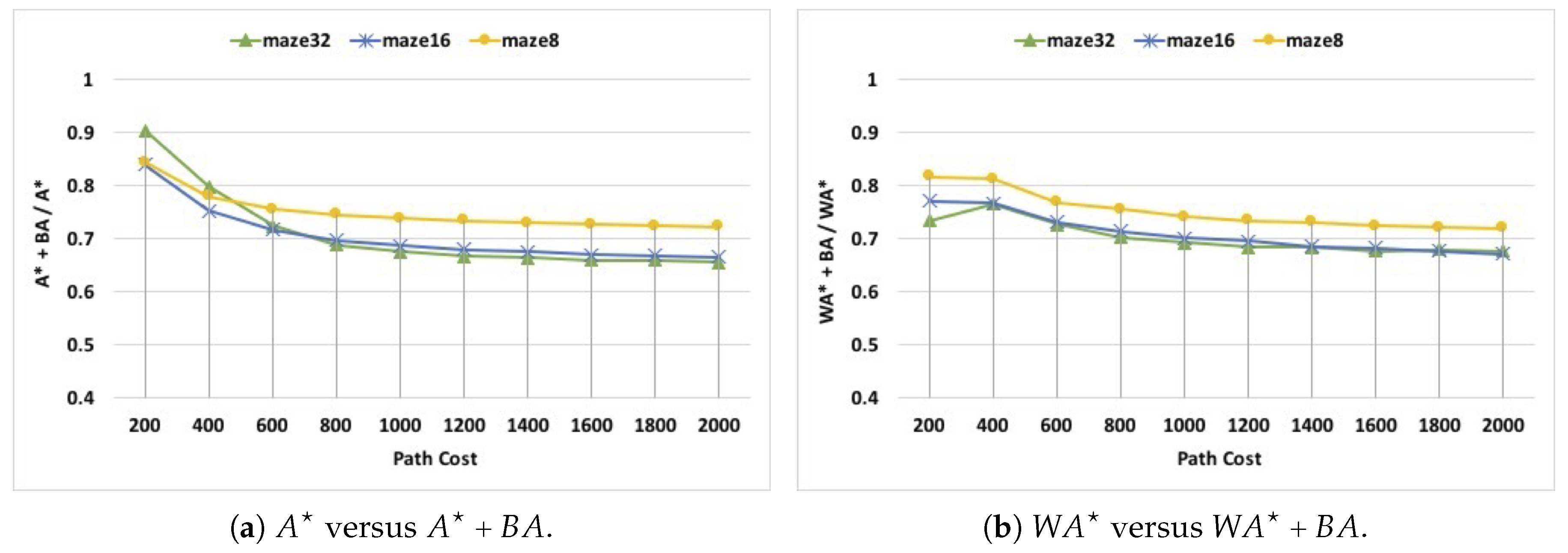
The performance results in Table 4 demonstrates that using blocked areas’ knowledge during pathfinding has significant impact on reducing search time in both $A^{★}$ and $W{A}^{★}$. However, Table 4 hides some of the interesting details about how the benefit of blocked areas’ knowledge compares between short-distance pathfinding versus long-distance pathfinding. For example, in mazes, there are thousands of pathfinding scenarios available from the pathfinding benchmarks library, in which some scenarios have short paths (i.e., path cost is less than 100), whereas some scenarios have long paths with cost up to 2000. Figure 6 demonstrates the impact of blocked areas’ knowledge on different path costs in mazes. Specifically, in Figure 6, we divide all scenarios into ten groups, where scenarios in the first group have path costs from 0 to 200, scenarios in the second group have path costs from 200 to 400, scenarios in the third group have path costs from 400 to 600 and so on. 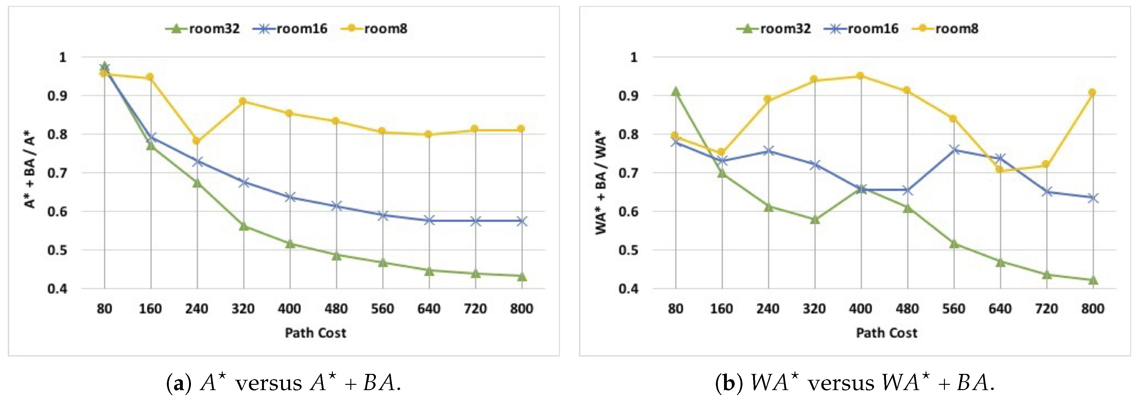Similarly, Figure 7 depicts the impact of blocked areas’ knowledge on different path costs in rooms. Note that, unlike mazes, scenarios in room maps have path costs that are between 0 and 800. Therefore, these scenarios are divided into ten groups, where scenarios in the first group have path costs between 0 and 80, scenarios in the second group have path costs between 80 and 160, scenarios in the third group have path costs between 160 and 240 and so on.

Figure 6. Relative execution times across different path costs in mazes.

Figure 7. Relative execution times across different path costs in rooms.

Figure 6 shows that, in all three types of mazes, blocked area’s knowledge has significant but different performance impacts on both short-distance and long-distance pathfinding. Specifically, in $A^{★}$, the execution time is reduced by $10\%$ for low path costs, and then this reduction steadily improves as the path cost increases, to reach around 35%, for high path costs. In $W{A}^{★}$, the reduction in execution time varies from $18\%$ in low path costs to $34\%$ in high path costs.

Figure 7 shows that, in all three types of rooms, the impact of blocked area’s knowledge on performance is mostly significant in both short-distance and long-distance pathfinding. However, this impact differs across different room types. In $A^{★}$, in the case of room-32, the reduction in execution time starts from a moderate $3\%$, and then sharply improves as the path cost increases to reach $57\%$ for paths with high costs. In room-16, the reduction in execution time starts from $3\%$ in low path costs and quickly increases to reach $43\%$ in high path costs. In room-8, the reduction in execution time gradually increases from $5\%$ in low path costs to $19\%$ in high path costs. In $W{A}^{★}$, the performance behavior is less deterministic, i.e., in some cases the reduction in execution time decreases as the path cost increases. However, this nondeterminism varies in degree between different types of rooms. In room-32, the reduction in execution time starts form $10\%$ for low path costs and then sharply improves to reach $58\%$ in high path costs (with the exception of one case). In room-16, the reduction in execution time varies between $23\%$ and $36\%$ while having less consistent behavior. In room-8, the reduction in execution time varies between $6\%$ and $30\%$ while also having no consistent trend in performance.

We summarize the results of our evaluation of pathfinding in mazes and rooms as follows. In all three types of mazes, in general, the execution times of both $A^{★}$ and $W{A}^{★}$ were reduced by 10–$35\%$ (the average reduction is $28\%$). In all three types of rooms, in general, the execution times of both $A^{★}$ and $W{A}^{★}$ were reduced by 5–$57\%$ (the average reduction is $30\%$). Unlike mazes, different room map types have significantly different degrees of how many nodes are covered by blocked areas, which led to having different performance behaviors.

Finally, it is worthwhile to mention that eliminating nodes inside blocked areas during pathfinding often led $A^{★}+BA$ to find a different path from the one found by $A^{★}$. However, in all maps and in all scenarios, both paths had the same optimal cost (as was also proven in Section 4). In the case of $W{A}^{★}+BA$ and $W{A}^{★}$, both algorithms found sub-optimal paths. In most cases, the two paths obtained by both algorithms have the same cost. However, interestingly, in some cases, we observed that $W{A}^{★}+BA$ found paths with lower costs than $W{A}^{★}$. This is because the exploration of blocked areas led $W{A}^{★}$ in some cases to find a longer path. On average, $W{A}^{★}+BA$ reduces the path cost of $W{A}^{★}$ by $2\%$.

8. Conclusions

This paper introduced the concept of blocked areas, which are sub-regions in grid maps where there is no viable path due to obstacles. In the context of grid-based optimal or sub-optimal pathfinding, the presence of blocked areas causes heuristic search algorithms to frequently explore irrelevant paths, significantly increasing search time in the process. To decrease search time, this paper presented a preprocessing approach that uses computational geometry techniques to identify blocked areas with polygon shapes in a grid map and store information about them into a memory-efficient balanced binary search tree. During actual pathfinding, the stored knowledge about blocked areas is used to avoid exploring paths inside blocked areas, which in turn reduces search time.

We evaluated the performance by comparing the execution times of $A^{★}$ and $W{A}^{★}$ before and after using blocked areas’ knowledge in pathfinding for a publicly available benchmark set that includes sixty maps of mazes and rooms. Our experimental results have shown that the execution times for both $A^{★}$ and $W{A}^{★}$ have been substantially decreased while preserving the optimality of $A^{★}$ and the sub-optimality of $W{A}^{★}$. This is achieved for both short-distance and long-distance pathfinding. Furthermore, we calculated the worst-case bounds for the memory needed to store blocked areas’ information during preprocessing and the access time needed to retrieve this information during pathfinding and showed that those bounds are efficient.

Utilizing blocked areas’ knowledge during pathfinding is applicable beyond the $A^{★}$ and $W{A}^{★}$ algorithms. In future work, we will study the impact of combining blocked areas’ knowledge with other search algorithms in the literature.