Article

Prediction of Tool Point Frequency Response Functions within Machine Tool Work Volume Considering the Position and Feed Direction Dependence

1
College of Mechanical Engineering, Chongqing University, Chongqing 400030, China
2
School of Advanced Manufacturing Engineering, Chongqing University of Posts and Telecommunications, Chongqing 400065, China
3
Chongqing Machinery and Electrical Holding (Group) Co. Ltd., Chongqing 401123, China
*
Author to whom correspondence should be addressed.
Symmetry 2020, 12(7), 1073; https://doi.org/10.3390/sym12071073
Submission received: 17 June 2020 / Revised: 26 June 2020 / Accepted: 27 June 2020 / Published: 30 June 2020

Abstract

:
A chatter vibration in milling process results in poor surface finish and machining efficiency. To avoid the chatter vibration, the stability lobe diagram (SLD) which is the function of tool point frequency response functions (FRFs) is adopted to predict the chatter-free machining parameters. However, the tool point FRF varies with the changes of machining positions and feed directions within machine tool work volume. Considering this situation, this paper presents a method to predict the position and feed direction-dependent tool point FRF. First, modal parameters of the tool point FRFs obtained at some typical positions and feed directions are identified by the modal theory and matrix transformation method. With the sample information, a back propagation (BP) neural network whose inputs are the position coordinates and feed angle and outputs are the modal parameters can be trained with the aid of the particle swarm optimization (PSO) algorithm. Then, modal parameters corresponding to any position and feed direction can be predicted by the trained BP neural network and used to reorganize the tool point FRFs with the modal fitting technique. A case study was performed on a real vertical machining center to demonstrate the accurate prediction of position and feed direction-dependent tool point FRFs. Furthermore, the position and feed direction-dependent milling stability was researched and origin-symmetric distributions of the limiting axial cutting depths at each machining position were observed.

1. Introduction

Self-excited vibration occurring in the milling process of machine tool is the key factor that results in worsening the machined surface quality, limiting the productivity, deteriorating tool wear and shortening machine tool service life span [1,2,3]. Generally, the stability lobe diagram (SLD) has been proposed to select appropriate chatter-free machining parameters. To plot the SLD, frequency response functions (FRFs) at the tool point should be obtained in advance [4,5,6]. However, since the machine tool spatial structure and the joints contact positions will vary with the movements of the machine tool moving parts, such as the spindle system and worktable, the tool point FRFs are not constant in the machine tool work volume and result in uncertain SLD predictions. Therefore, further research has been developed to predict the position-dependent tool point FRFs, and study variations of the milling stability in the machine tool work volume [7,8,9].
The tool point FRFs can usually be obtained through two approaches. One is the impact testing performed on real machine tool structure, and the other is the modal analysis performed on the mathematic model or finite element model (FEM) in virtual environment [10,11]. Luo et al. [12] considered the influence of machine tool structure change on the tool dynamic properties and proposed a mathematic model to predict the natural frequency by modifying the mass matrix. However, this research has not mentioned how to obtain the tool point FRFs when the machine tool structure varies. Law et al [13] proposed a substructurally synthesized reduced order machine model to realize the theoretical rapid prediction of the position-dependent tool point FRFs by reconstructing the machine tool dynamic model at each position, and then the milling stability for different combinations of machining positions and feed directions were analyzed. Tunc et al. [14] measured the tool tip FRFs at different machining positions and along different feed directions, and these FRFs were further used to plot the SLDs to determine the optimal feed direction to increase the chatter-free material removal rate.
Since the aforementioned methods are still time-consuming and it is difficult to reconstruct the machine tool real structure or FEM to measure or simulate the machine tool dynamics at each machining position, some researches combining the approximate model and experimental design method have been proposed. Baumann et al. [15] determined 23 positions in the machine tool workplace to measure the dynamics of the spindle, and then a triangle-interpolating model was established to predict the dynamics of the spindle at other positions. Deng et al. [16] obtained FRFs of the machine tool frame-holder base at 27 sample positions, and then a Kriging model whose inputs were the moving parts displacements in x, y and z directions was established. And in addition, the predicted FRFs at the base points were further used to predict the FRFs for different tools based on the receptance coupling substructure analysis (RCSA). Similarly, considering the different tool-holder assemblies, Liu and Chen et al. [17,18] used transfer learning to predict the pose-dependent tool tip dynamics by integrating domain adaptation and adaptive weighting. Once the pose-dependent tool tip dynamics were obtained by sufficient impact tests, only few impact tests to measure the new tool tip dynamics were required.
Majority of researches discussed the effects of the varying machining positions on the tool point FRFs and the machining stability. However, the feed direction which also affects the tool point dynamics has been addressed little. Besides the aforementioned research developed by Law and Tunc, Yang et al. [19] investigated the SLDs with different spindle positions and feed directions based on the modal tests. And in addition, the performed cutting tests also validated that the machining stability differences caused by the feed directions. However, these methods are still time-consuming to investigate the position and feed direction-dependent milling stability within whole machine tool work volume.
Therefore, this paper proposes a method to predict the tool point FRFs at any machining position and feed direction without complicated impact modal experiments. First, typical machining position and feed direction combinations are determined to obtain the related tool point FRFs with the modal tests and matrix transformation method; then the sample position coordinates and feed angles are taken as the input information and related modal parameters are taken as the output information to train a BP neural network with the aid of the PSO algorithm; thus, the trained and validated BP neural network can be used to predict modal parameters at other combinations of machining position and feed direction, which are further used to reorganize the corresponding tool point FRFs with the modal fitting technique. Then reorganized tool point FRFs are utilized to plot stability lobe diagrams to investigate the position and feed direction-dependent machining stability.
Henceforth, this paper is organized as follows. The principles of the proposed method for predicting the position and feed direction-dependent tool point dynamics are provided in Section 2. In Section 3, a case study describing the application of the proposed PSO-BP method is performed on a real vertical machining center. The position and feed direction-dependent machining stability is investigated through some case studies in Section 4. Finally, conclusions from the current research are summarized in Section 5.

2. Theoretical Background

Three steps are defined to efficiently predict the position and feed direction-dependent tool point FRFs. First, the modal theory and matrix transformation are combined to obtain the FRFs considering feed directions and identify the corresponding modal parameters. Then, with the information of machining position, feed direction and modal parameters, the particle swarm optimization algorithm is used to benefit the training of the BP neural network. Finally, the trained network is used to predict the position and feed direction-dependent modal parameters, and the related tool point FRFs are reorganized by using the modal fitting technique. A flowchart for describing the aforementioned whole research is provided in Figure 1.

2.1. Modal Theory and Matrix Transformation

According to the modal theory, the frequency response function can be expressed as a superposition of multiple single modes. When the excitation force is applied to the system at point p, the vibration response at point l is described as follows [20]:
H l p ( ω ) = r = 1 N 1 K e r [ ( 1 λ r 2 ) + j 2 ξ r λ r ] ω r = K e r / M r λ r = ω / ω r ξ r = C r / 2 M r K e r = C r / 2 M r ω r
where ωr, ξr, Mr and Ker are the rth modal natural frequency, damping ratio, mass and stiffness respectively.
If the system vibrates near the rth mode, the dynamic response can be obtained by Equation (2):
H l p ( ω ) ω = ω r = 1 K e r [ ( 1 λ r 2 ) + j 2 ξ r λ r ]
Then the real and imaginary parts of the frequency response function in Equation (2) can be written as follows.
Real [ H l p ( ω ) ] ω = ω r = 1 K e r [ 1 λ 2 ( 1 λ 2 ) 2 + ( 2 ξ r λ ) 2 ] Im a g [ H l p ( ω ) ] ω = ω r = 2 ξ r λ K e r [ ( 1 λ 2 ) 2 + ( 2 ξ r λ ) 2 ]
According to Equation (3), the maximum real part value occurs when λ r t h max = 1 2 ξ r , and λrthmax can be equal to (1 − ξr) if ξr2 is ignored; the minimum real part value occurs when λ r t h min = 1 + 2 ξ r , and λrthmin can be equal to (1 + ξr) if ξr2 is ignored. Therefore, the vibration frequencies corresponding to the maximum and minimum real part values are ω1r = ωr(1 − ξr) and ω2r = ωr(1 + ξr) respectively, and then the ξr can be obtained by ω1r and ω2r using the following Equation (4).
ξ r = ω 2 r ω 1 r 2 ω r
For the imaginary part in Equation (3), its minimum value occurs when λrthimin = 1, and the corresponding vibration frequency ωr and amplitude Ar are represented in Equation (5).
ω = ω r K e r = 1 2 ξ r A r
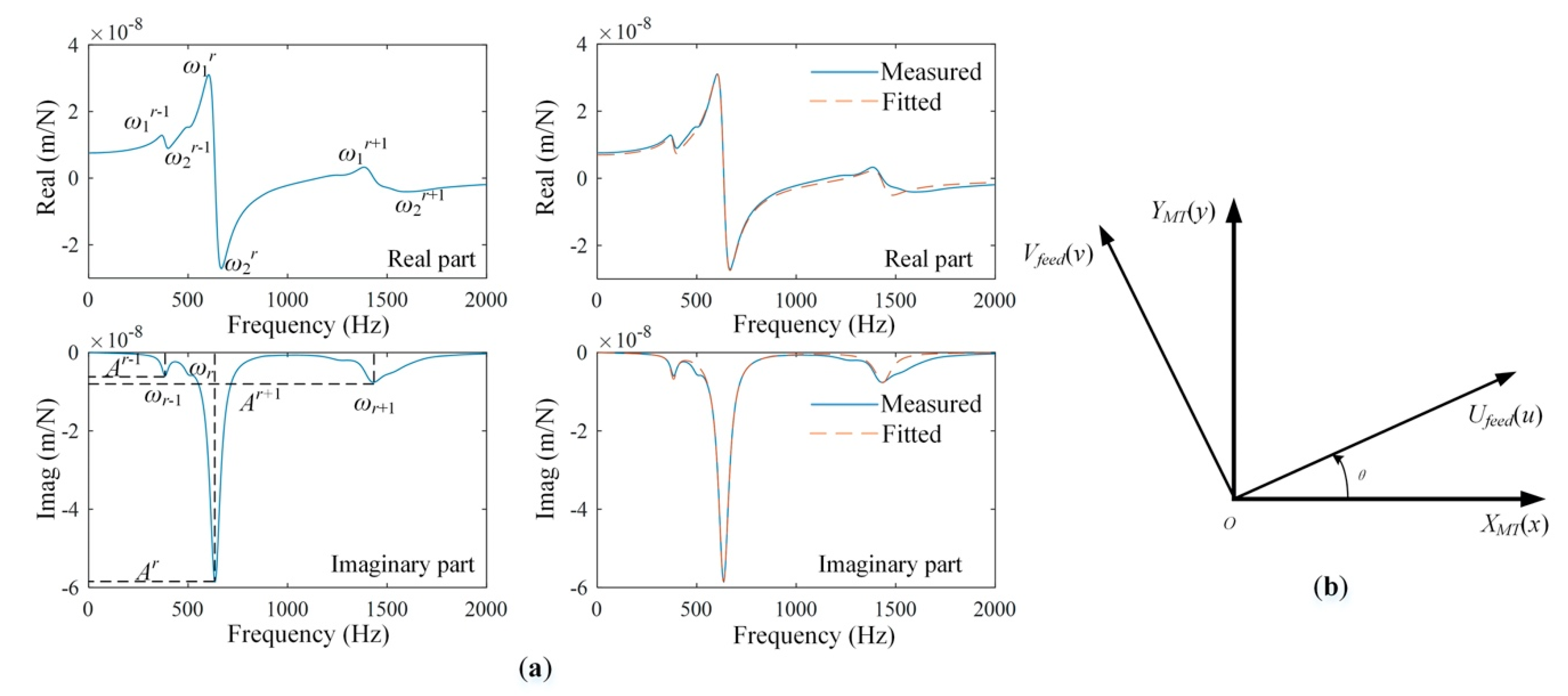
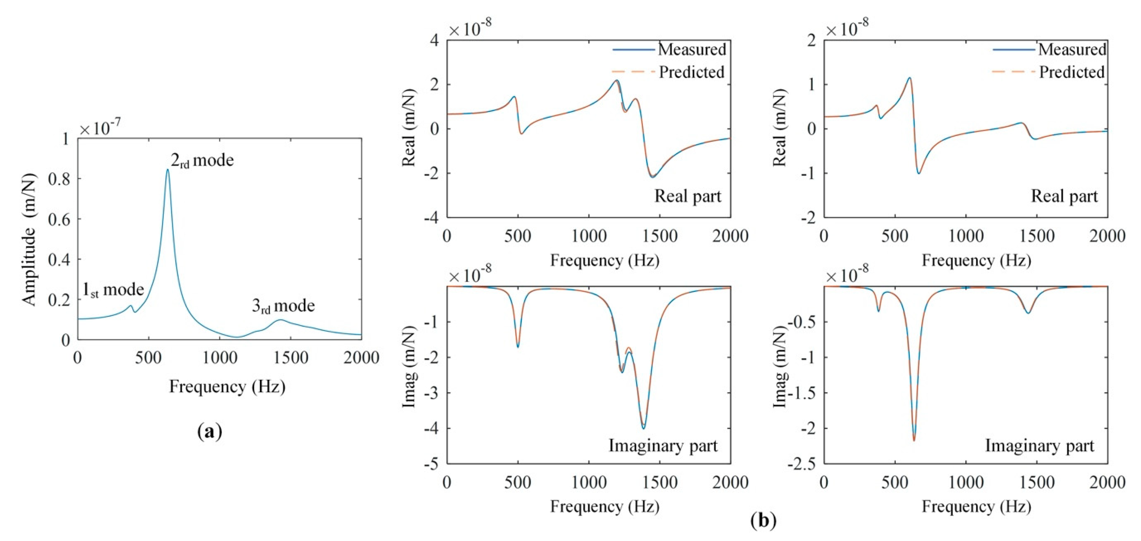
Accordingly, once a frequency response function curve is obtained through impact testing or virtual simulation, the modal parameters for each mode can be identified according Equations (4) and (5). The real and imaginary parts of a measured FRF curve are taken as an instance to describe the identification process. The ω1r, ω2r and Ar for each mode are labeled in Figure 2a and used to identify related modal parameters. The identified modal parameters are used to reorganize the measured FRF and well consistence is observed in Figure 2a.
Generally, the horizontal (x) and normal (y) axes are used to define a machine tool coordinate system (XMT and YMT) shown in Figure 2b, and the x and y directional tool point FRFs in the machine tool coordinate system are measured to analyze vibrations in related directions. The direct and cross FRFs at the tool point in x and y directions compose the frequency response function matrix Gxy described in Equation (6). However, in real machining process, the feed direction is not always consistent with the x and y axes defined in machine tool coordinate system (XMT and YMT). Therefore, based on the machine tool coordinate system, a rotation angle θ and the feeding directions (u and v) are defined to establish a feed direction coordinate system (Ufeed and Vfeed) as shown in Figure 2b.
According to the relationship between the machine tool and feed direction coordinate systems, the frequency response function matrix Gxy in machine tool coordinate system is modified by a transformation matrix R described in Equation (6) to obtain the frequency response function matrix Guv in feed direction coordinate system [13,21]. Therefore, if the position-dependent matrix Gxy is measured or simulated, it can be further used to calculate the position and feed direction-dependent matrix Guv with Equation (6).
G x y ( i ω ) = [ H x x H x y H y x H y y ] G u v ( i ω ) = [ H u u H u v H v u H v v ] = R 1 G x y ( i ω ) R = [ cos θ sin θ sin θ cos θ ] 1 G x y ( i ω ) [ cos θ sin θ sin θ cos θ ]

2.2. BP Neural Network and PSO Algorithm

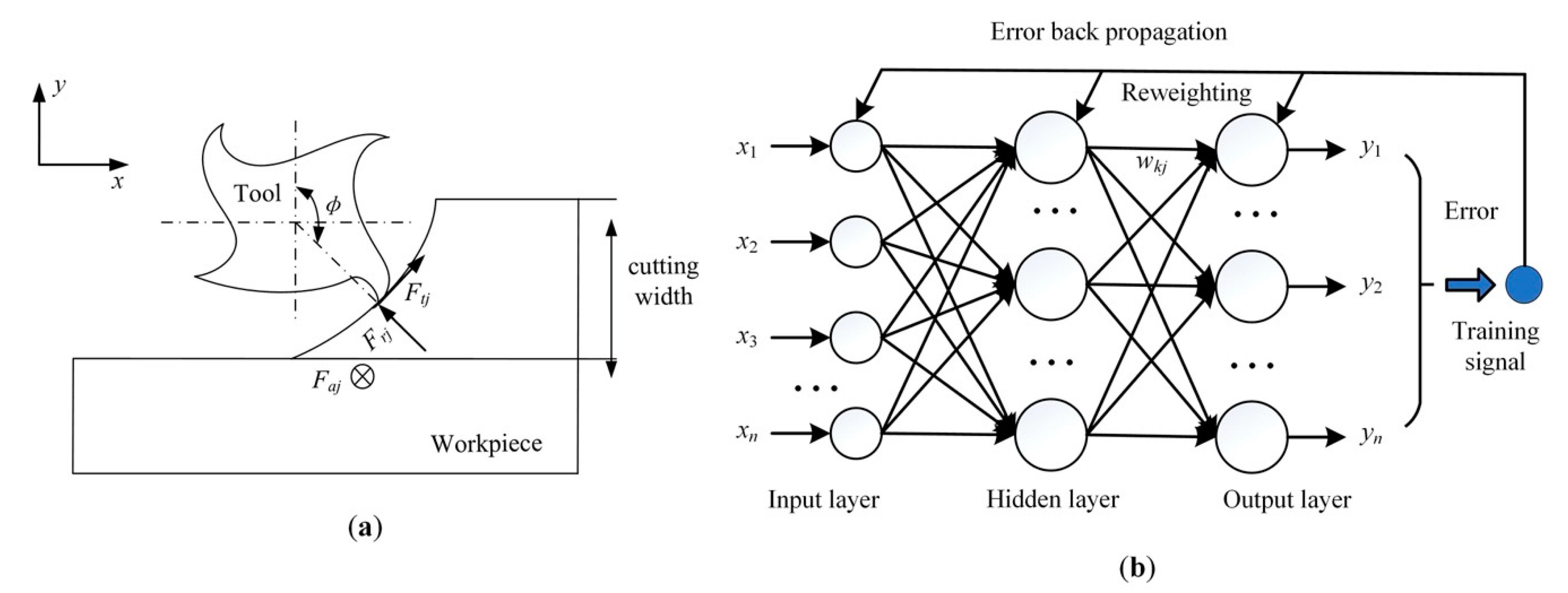
A two degree of freedom (DOF) dynamic model shown in Figure 3a is usually established to describe the milling process. In addition, the milling stability is analyzed based on a modal model of the machine and the following characteristic equation [22,23].
det ( [ I ] + Λ [ G 0 ( i ω c ) ] ) = 0 Λ = ( Λ R + Λ I i ) = 1 4 π N t K t a p ( 1 e i ω c T )
where ΛR and ΛI are the real and imaginary parts of the complex eigenvalue Λ, Nt is the tool tooth number, Kt is the tangential cutting force coefficient, ap is the axial cutting depth, ωc is the chatter frequency and T is the tooth passing period determined by the spindle speed n. The G0(c) is the directional matrix can be written as Equation (8).
G 0 ( i ω c ) = [ A ] G u v ( i ω c )
Then, with Equations (7) and (8), the limiting axial cutting depth considering the feed direction aplim-feed and the related spindle speed n can be analytically calculated using Equation (9).
a p lim f e e d = 2 π Λ R f e e d N t K t [ 1 + ( Λ I f e e d Λ R f e e d ) 2 ]   n = 60 ω c N t [ ( 2 k + 1 ) π 2 tan 1 ( Λ I f e e d / Λ R f e e d ) ]
According to Equations (7) to (9), the prerequisite to determine the milling stability within the machine tool work volume is obtaining the position and feed direction-dependent Guv. Since the matrix Guv is composed by the tool point FRFs, its variations can be represented by the variations of the corresponding FRFs. Considering that the FRFs are organized by the modal parameters as described in the aforementioned Section 2.1, variations of the tool point FRFs can be represented by the variations of modal parameters, and further ascribed to the position and feed direction changes. Therefore, a mathematic model needs to be established to predict the modal parameters at any combination of machining position and feed direction.

2.2.1. BP Neural Network

Since the BP neural network can theoretically approximate any nonlinear continuous function with reasonable topological structure and appropriate structure parameters, it is selected to establish the mathematic model for predicting the position and feed direction-dependent modal parameters [24]. Figure 3b shows a three layer BP neural network, and it makes use of error gradient descent algorithm to minimize the mean square error between the actual output value and the output value predicted by network.
As shown in Figure 3b, each layer is composed by a single or multiple neurons, and the neurons in adjacent layers are connected by the linking weights. The input layer contains the input variable X = [x1, x2,…,xm], and its neurons number equals the number of input variables. The output layer contains the output variable vector Y = [y1, y2,…,yt], and its neuron number equals the number of output variables. Since this paper aims to obtain the modal parameter at any position and feed direction, the displacements of the moving parts in x, y and z directions and the feed angle θ described in Figure 2b are taken as the inputs of the BP neural network, and the modal parameters are taken as the outputs of the BP neural network. The neurons number in the hidden layer usually determined according to the empirical equation:
l = m + t + a
where m and t are the number of neurons in the input and the output layer respectively, and a is an arbitrary integer number between 1 and 10.
For the neuron in hidden or output layer, its output can be calculated by the following Equation (11).
O i k = f ( j = 1 m w k j O i 1 j + ψ i k )
where Oik is the output of the kth neuron in ith layer, f(·) is the excitation function, wkj is the linking weight between the jth neuron in i − 1th layer and the kth neuron in ith layer, Ψik is the threshold of the kth neuron in ith layer. The linking weight is modified based on the error function descried by the actual and predicted output values in Equation (12).
Δ w k j = η E w k j E ( X ) = q = 1 t ( y a q ( x ) y p q ( x ) ) 2
where Δw is the linking weight adjustment, η is the constant between 0 and 1 reflecting the learning rate of the BP neural network, and yaq and ypq are the qth actual and predicted output value respectively.
Therefore, if the basic parameters for establishing a BP neural network are determined, such as the neuron number for each layer, the linking weight between each pair of neurons, the threshold value of each neuron, learning rate for the back training algorithm and so on, the BP neural network can be trained to approximate the mathematic relationship between the input and output values.

2.2.2. Particle Swarm Optimization Algorithm

BP neural network has the advantage in approximating the nonlinear relationship between the inputs and outputs, but it shows slow training speed and is easy to fall into the local minimum in the training process. To overcome these shortcomings, the particle swarm optimization algorithm and the genetic algorithm (GA) have been first selected to determine the structure parameters of the BP neural network, and the BP neural network trained with the aid of PSO algorithm has shown higher prediction accuracy. Thus, the particle swarm optimization algorithm which has the advantages of fast convergence, strong robustness and global search ability is finally selected in this paper to help training the BP neural network [25,26].
In the D-dimensional search space, m particles form a population. For each particle, it has two attributes including the position and velocity. For the ith particle, its position vector can be expressed as Xi = (xi1, xi2,…,xiD). During the searching process, each current particle position is a candidate solution to the corresponding optimization problem, and the fitness function is determined to judge the historical optimal position of each particle and the historical optimal position of the population. Each current individual optimal position and the global optimal position are further used to determine the corresponding velocity vector of each particle. For the ith particle, the determined velocity vector Vi = (vi1, vi2,…,viD) is used to modify the current particle position to close to the historical optimal one. Then, the new position for each particle is obtained to continue the next iteration. During the iteration, the position and velocity of each particle are repeatedly updated using the following Equation (13). The iteration terminates until the best global fitness value or the total iteration number meets the termination condition.
v i d k + 1 = ω v i d k + c 1 r 1 ( p i d x i d k ) + c 2 r 2 ( p g d x i d k ) x i d k + 1 = x i d k + v i d k + 1 i = 1 , 2 , , m ;   d = 1 , 2 , , D
where k is the current iteration number, ω is the inertia weight, c1 and c2 are the acceleration factors, r1 and r2 are the random numbers between 0 and 1.
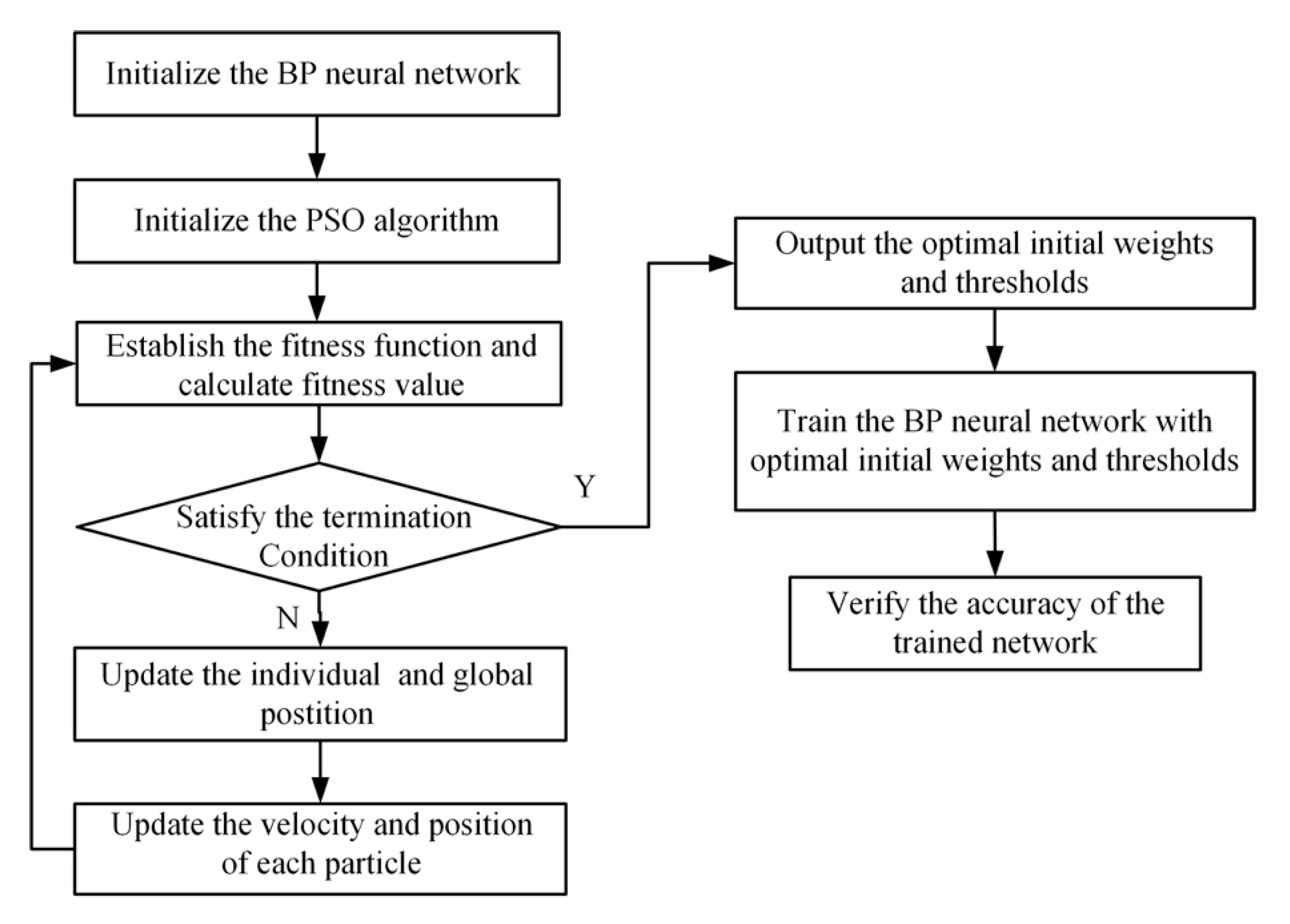
In order to establish the BP neural network with the aid of PSO algorithm, the weights and thresholds are taken as the particles. Then positions and velocities of the particles are updated iteratively to realize the optimal positions. The application flow chart of the combined BP neural network and PSO algorithm for predicting the position and feed direction-dependent modal parameters is shown in Figure 4, and the related procedures are summarized as follows.
Step 1: Initialize the BP neural network. Define the neuron numbers of the input layer, hidden layer and output layer according to Section 2.2.1, and normalize the input and output sample data between −1 and 1. Other basic parameters should also be determined, such as the learning rate, excitation function, training goal and so on.
Step 2: Initialize required parameters of the PSO algorithm. First, the particle dimension D is determined by the total number of the weights and thresholds using Equation (14).
D = N i n p u t × N h 1 + i = 1 N h t N h i + N h m × N o u t p u t + i = 1 m N h i + N o u t p u t
where Ninput and Noutput are the neuron numbers in the input and output layers, Nht is the total number of hidden layers, and Nhi is the neuron number of the ith hidden layer. Then, the population size, iteration number, inertia weight, initial positions and velocities, acceleration factors, and rand numbers are initialized. Moreover, the lower and upper boundaries of these positions and velocities are also defined. The error function described in Equation (12) is taken as the fitness function.
Step 3: Obtain the optimal initial weights and thresholds of the BP neural network. During each iteration of the PSO algorithm, the individual and global optimal positions are updated and recoded by comparing the so far calculated particle fitness values, and the corresponding individual and global optimal fitness values are also updated and recoded. When the iteration terminates, the global optimal position is taken as the optimal initial weights and thresholds to train the BP neural network according to Section 2.2.1. In addition, the accuracy of the trained BP neural network is verified by the testing sample including the information of the input and output variables.

3. Case Study

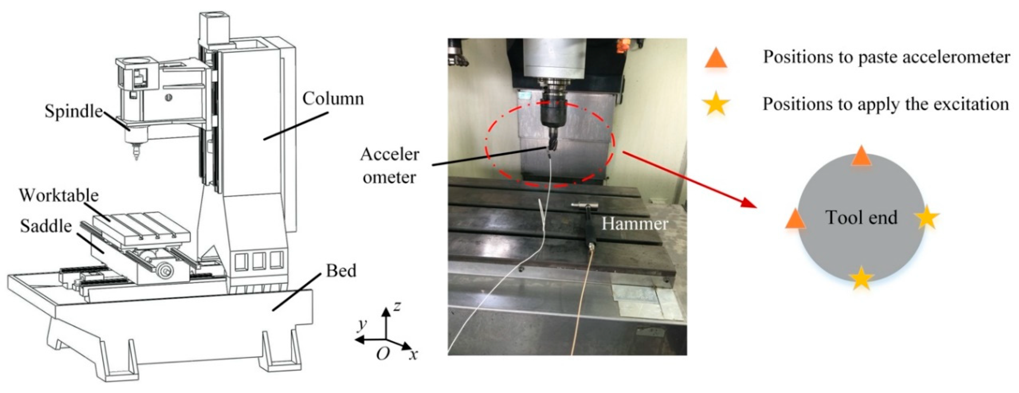
In this section, the proposed BP-PSO method for predicting the position and feed direction-dependent tool point FRFs was applied to a real three-axis vertical machining center shown in Figure 5, the worktable, saddle and spindle system of which move along the x, y, and z directions respectively. The movement ranges of the worktable, saddle, and spindle system are 0–550 mm, 0–400 mm and 0–400 mm respectively, and the corresponding displacements of the three axes are combined to represent the machining position.

3.1. Impact Testing Based on Orthogonal Experiment Design

To establish the BP neural network for predicting the tool point FRFs within the machine tool work volume, the commonly used orthogonal experimental design is first introduced to determine some representative sample machining positions and feed directions. The orthogonal experimental design has the characteristics of uniform distribution and good comparability, and it can benefit obtaining the typical position and feed direction-dependent tool point FRFs with fewer modal experiments [27]. Then, the displacements in x, y and z directions and the feed direction angle θ are taken as the factors, and eight levels for each factor are determined within its variation range. The corresponding factors and levels are listed in Table 1, and an orthogonal table L64(84) is used to determine 64 experiment schemes shown in Table 2.
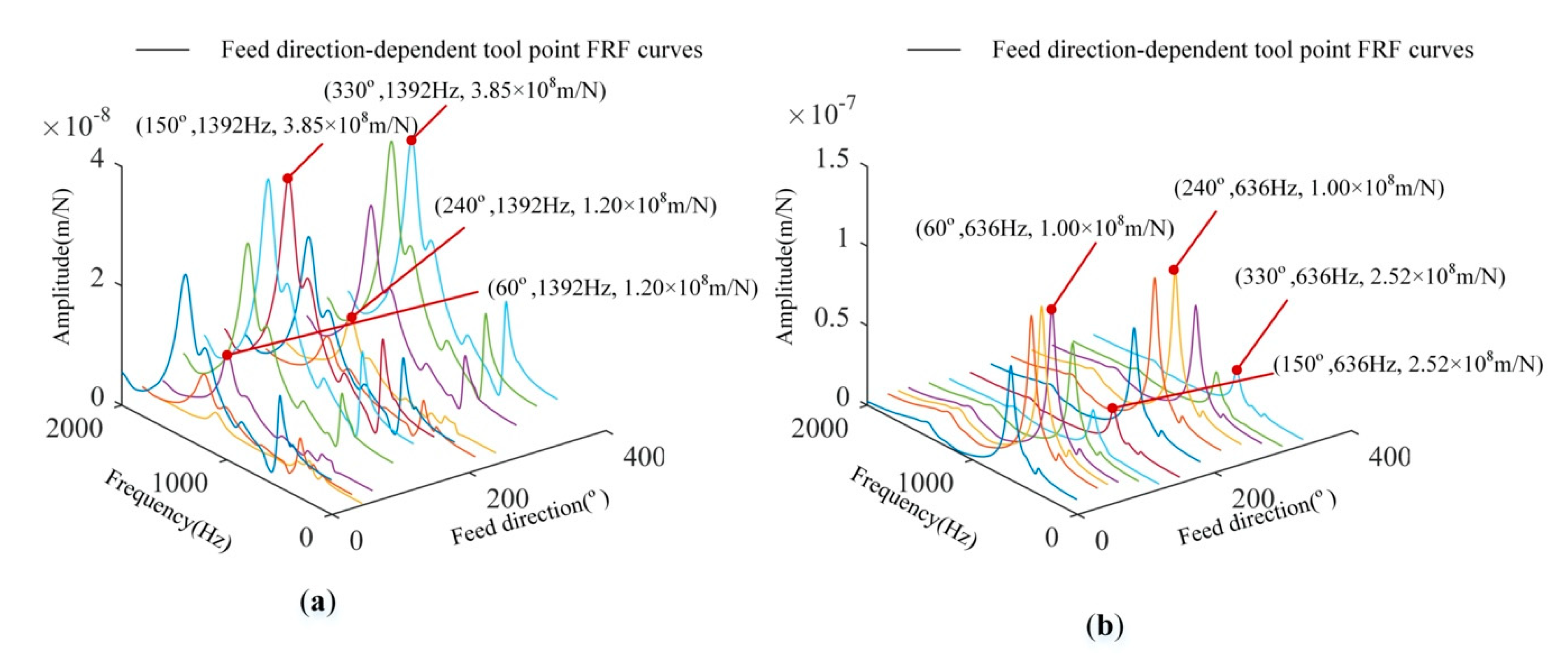
The first four columns of Table 2 represent the typical combinations of machining position and feed direction. At each combination, the worktable, saddle, and spindle system are driven to achieve the machining position, and the impact testing was performed at the tool point of each machining position. During the experiment, the impact hammer with the type PCB 086D05, sensibility 0.23 mv/N and weight 0.32 Kg exerted the excitations and recorded the force signals at the tool point in x and y directions, and the accelerometer with the type PCB-ICP, sensibility 99.6 mv/g and weight 4.0 g was pasted to the tool point to measure the acceleration response signals as shown in Figure 5 [28]. Then, the x and y directional tool point frequency response functions at these typical machining positions were obtained, which were further used to calculate the tool point FRFs considering the position and feed direction simultaneously by Equation (6). For instance, at one fixed machining position, the tool point FRFs for different u and v directions are plotted in Figure 6, and these FRFs show an origin-symmetric phenomenon. For example, in Figure 6a, when the natural frequency is 1392 Hz, the corresponding amplitudes for feed direction angles θ = 60° and θ = 240° are 1.20 × 10⁻⁸ m/N and for feed direction angles θ = 150° and θ = 330 ° are 3.85 × 10⁻⁸ m/N; in Figure 6b, when the natural frequency is 636 Hz, the corresponding amplitudes for feed direction angles θ = 60° and θ = 240° are 1.00 × 10⁻⁷ m/N and for the feed direction angles θ = 150° and θ = 330° are 2.52 × 10⁻⁸ m/N. Thus, effects of the feed direction variations on tool point FRFs can only consider the feed direction angle within the range [0°, 180°].

3.2. BP-PSO Method for Modal Parameters Prediction

With the obtained machining position and feed direction-dependent tool point FRFs in Section 3.1, corresponding modal parameters can be identified according to Equations (4) and (5). Analyzing these tool point FRF curves, three obvious modes for each curve can be observed, and then the natural frequencies, modal stiffnesses and modal damping ratios for the three modes were identified. One FRF in v direction is taken as an example in Figure 7a, and the identified modal parameters are listed in Table 3. Considering the u and v directions, the BP neural network should be established to predict the modal parameters of six modes. Predicting 18 modal parameters simultaneously will result in over-complicated structure and slow convergence speed. Therefore, six BP neural networks were established, and each neural network is used to predict the natural frequency, modal stiffness, and modal damping ratio of each mode. Then, the modeling process of a single BP neural network with the aid of PSO algorithm is described to give an illustration.
Taking the prediction of the second modal parameters of the tool point FRF in u direction as an instance, the input layer has 4 neurons, which represent the displacements of x, y and z directions and the feed direction angle θ; the output layer has 3 neurons, including the natural frequency ω, modal stiffness K and modal damping ratio ζ; one hidden layer is defined, and 3 neurons are determined according to Equation (10). Then, in the PSO algorithm, 100 particles are defined to compose one population, and each particle has 27 dimensions calculated according to Equation (14) and represents the initial linking weights and thresholds of the BP neural network; the fitness function is the mean squared errors between the real and predicted modal parameters; the minimum and maximum velocity are −0.5 and 0.5; the inertia weight variation range is defined as [0.4, 1.2], and the inertia weight is first defined as 1.2 and decreases with the iteration number linearly; the initial velocity vector of each particle was defined randomly, and the acceleration constants were 1.45.
According to Section 3.1, 64 combinations of three directional displacements and feed direction angle (x, y, z, θ) in Table 2 were defined as the input sample, and the corresponding 64 combinations of the modal parameters were taken as the output sample. Moreover, 58 combinations were selected randomly to be the training sample, and the other 6 combinations were determined as the testing sample. Then, the BP neural network was trained based on the PSO algorithm and the training sample. Using the testing sample to verify the prediction accuracy of the trained BP neural network, comparisons of the original and predicted modal parameters values for the testing sample are described in Table 4. Relatively small errors are observed, validating the accuracy of the trained BP neural network, which can be used to predict the position and feed direction-dependent modal parameters.
After the six BP neural networks were established and trained, the predicted 18 modal parameters can be further used to reorganize related position and feed direction-dependent tool point FRFs. Figure 7b is an example of the measured and predicted FRFs along u and v directions at one position, and good consistencies are observed. Therefore, the predicted position and feed direction-dependent tool point FRFs can be used to analyze the milling stability within the whole machine tool work volume.

4. Chatter Stability Analysis Considering Uncertain Position and Feed Direction

Main purpose of the milling stability prediction is selecting appropriate machining parameters to avoid the chatter vibration. Since the milling stability depends on the tool point FRFs which is a function of the machining positions and feed direction, the milling stability will vary in the whole machine tool work volume. Therefore, this section describes the position and feed direction-dependent milling stability simulation for downing milling the workpiece whose material is the commonly used ASTM 1045 steel with tool diameter 20mm and tooth number Nt = 4, tangential cutting force coefficient Kt = 1799 MPa and radial cutting force coefficient Kr = 760 MPa.
First, the left-most, middle and right-most positions of each direction are defined, and the feed direction-dependent milling stabilities related to the three positions were researched based on the Equations (7) to (9) and the established BP neural networks in Section 3. When the position of one moving part varies along one direction, no movements of the other two directions were defined. Taking the spindle speed 8400 rpm as an instance, the calculated axial limiting cutting depth aplim_feed values are plotted in Figure 8.
Figure 8a–c describe the aplim_feed value changing with the feed directions when the worktable, saddle and spindle system are at three positions along x, y and z directions respectively, and origin-symmetric distributions of aplim_feed values for each position are observed. In Figure 8a, when the feed direction angle varies from 0° to 360° at the three positions, the maximum and minimum aplim_feed values are 7.20 mm and 6.42 mm respectively, and the variation rate is 12.15%. In Figure 8b, the maximum and minimum aplim_feed values are 5.66 mm and 5.24 mm respectively, and the variation rate is 8.02%. In Figure 8c, the maximum and minimum aplim_feed values are 9.08 mm and 6.02 mm respectively, and the variation rate is 50.83%. Comparing three figures, Figure 8a,b show that aplim_feed values are mainly affected by the feeding directions, and the machining position variations in x and z directions show slight effects on the aplim_feed values; however, in Figure 8c, not only the feed direction variations but also the machining position variations have significant effects on the aplim_feed values. Thus, the machining position and feed direction should be considered when designing the process plan.
Furthermore, since the limiting axial cutting depth is affected by the tool passing period T which depends on the spindle speed n shown in Equation (7), the spindle speed was taken as a factor and its eight levels were determined and listed in Table 1; then, the first five columns of Table 2 were used to perform the milling stability analysis, and the calculated axial limiting cutting depth aplim_feed values are shown in Table 2. Thus, the range analysis and variance analysis described as follows were adopted to comprehensively study the effects of the machining position (x, y, z), feed directions θ and spindle speed n on the milling stability.
In the range analysis, the range R was calculated according to Equation (15), which were used to investigate the effect degree of each factor on the axial limiting cutting depth aplim_feed and determine the optimal level of each factor. A factor with higher range value indicates that it shows a greater effect on the aplim_feed [29].
R j = max ( k i j )     min ( k i j )
where Rj is the range value of the jth factor, kij is the sum of the aplim_feed values calculated using the ith level of the jth factor, i = 1, 2, …, m, j = 1, 2, …, n, and m and n are the level and factor numbers of the orthogonal table respectively.
In the variance analysis, the F-test was used to determine the effect degree of each factor on the axial limiting cutting depth aplim_feed, and the parameters needed to perform the F-test were calculated according to Equation (16) [30].
{ T = p = 1 N u m p x p , C T = T 2 / N u m p , Q T = p = 1 N u m p x p 2 , r = N u m p / m S S j = 1 r i = 1 m k i j 2 C T , S S T = Q T C T , S S e = S S T j = 1 n S S j d f T = N u m i j 1 , d f j = m 1 , d f e = d f T j = 1 n d f j S j = S S j / d f j , S e = S S e / d f e , F j = S j / S e  
where xp is the aplim_feed value calculated using the pth scheme designed in the orthogonal table, Nump is the total number of designed schemes, SSj is the sum of squared deviation of the jth factor, dfT is the total degree of freedom, dfj is the degree of freedom for the jth factor, Sj is the variance of the jth factor, and Fj is the F value of the jth factor. The significance level of each factor is determined by comparing the obtained F value with the standard F value (Fα(dfj, dfe)). When the significant level α is given, the standard value Fα(dfj, dfe) can be attained from the F-table in accordance with the degree of freedom [30]. If the F value is higher than the standard Fα value, the factor is regarded as significant. And in addition, the factor with a higher F value means that it has more evident impact on the aplim_feed.
Therefore, the information in Table 2 were used to perform the range analysis and variance analysis with the Equations (15) and (16). Comparing the kij value of each factor listed in Table 5, the level with a higher kij value is regarded as the optimal level of the related factor. Thus, the 4th, 4th, 1st, 6th, 8th levels of the factor x, y, z, θ and n are determined as the optimal combination to have a bigger aplim_feed, and specific values of the subscripts are listed in Table 1. For the variance analysis, the calculated SST is 1029.10, SSe is 83.31, dfT is 63, dfe is 28, and other corresponding parameters are listed in Table 5. In this current research, the significant level α is defined as 0.05, and the obtained standard F values Fα are listed in Table 5. Comparing the F and Fα values of each factor listed in Table 5, the F values of the spindle speed n, z directional displacement, feed direction angle θ and x directional displacement are bigger than the F0.05(7, 28) = 2.359, which indicates that these four factors have significant effects on aplim_feed with a confidence level of 95%. Further comparing the F values of the five factors, the influence degree of the machining position (x, y, z), feed directions θ and spindle speed n on axial limiting cutting depth aplim_feed is n > z > θ > x > y. Analyzing the R and F values in Table 5, the spindle speed shows the dominant effects on the aplim_feed, the displacement in z direction and the feed direction angle θ have similarly significant effects on the aplim_feed, the displacement in x direction shows less evident influence on the aplim_feed, and the displacement in y direction has no evident effect on the aplim_feed. Accordingly, when designing the tool path, an optimal combination of z directional position and feed direction needs to be determined, and the movements in x and y directions should be first taken into consideration.

5. Conclusions

Considering the machining position and feed direction have significant effects on the tool point FRFs and thus on the milling stability, this paper proposes a method for predicting the machining position and feed direction-dependent tool point FRFs based on the modal theory, matrix transformation, BP neural network and PSO algorithm. The feasibility of the proposed method was verified by case studies on a real vertical machining center.
(1)
The displacements of the worktable, saddle and spindle system along the x, y and z directions represents the machining position, and the feed direction is represented by the rotation angle θ around the machine tool coordinate system. 8 levels of each factor were determined within its variation range, and then an orthogonal table with 64 schemes was designed. For each scheme, the machine tool was driven to the related spatial structure to measure the x and y directional tool point FRFs, and the matrix transformation method was used to calculate the related FRFs in u and v directions.
(2)
Three obvious modes for each tool point FRF were observed, and the related modal parameters were identified according to modal theory. Thus, considering the u and v directions, 18 modal parameters should be predicted for one machining position and feed direction combination. To avoid the complex training process and improve the convergence speed, 6 BP neural networks were established for predicting the modal parameters of six modes respectively. Then these BP neural networks were trained with the information of the randomly selected 58 schemes from the Table 2 and the optimized initial linking weights and thresholds using the PSO algorithm. The accuracies of established BP neural networks were verified by the measured modal parameters related to the combinations of machining position and feed direction included in the testing sample.
(3)
Moreover, these BP neural networks were used to research the milling stability within the machine tool work volume. Distributions of the axial limiting cutting depth within the feed direction angle range [0°, 360°] at 9 selected machining positions show that the z directional displacement and feed direction θ have significant effects on the limiting axial cutting depth. The same phenomenon was also observed from results of the range analysis and variance analysis performed according to the information in orthogonal Table 2. The optimal level for each factor was determined to obtain an optimal combination of machining position and feed direction with higher limiting axial cutting depth.
Therefore, the proposed method for predicting the machining position and feed direction-dependent FRFs can benefit an optimal process planning according to real milling conditions at the design stage. In further research, the proposed method can be extended to take more factors into consideration, such as the spindle speed and tool change, to make the FRFs prediction more fit in with the actual milling process.

Author Contributions

Funding acquisition, C.D.; investigation, Y.F. and J.S.; methodology, C.D. and Y.F.; software, Y.F. and J.S.; experiment, C.D. and Q.T.; writing—original draft preparation, C.D., Y.F. and Q.T.; writing—review and editing, C.D., Y.F. and Z.H.; supervision, C.D. All authors have read and agreed to the published version of the manuscript.

Funding

This research was funded by the National Natural Science Foundation of China under Grant no. 51705058, the China Postdoctoral Science Foundation funded project under Grant no. 2018M633314, and the Chongqing Special Postdoctoral Science Foundation under Grant no. XmT2018040.

Conflicts of Interest

The authors declare no conflict of interest.

Nomenclature

ωrrth modal natural frequency (Hz)
ξrrth modal damping ratio (%)
Mrrth modal mass (kg)
Kerrth modal stiffness respectively (×109 N/m)
Arrth amplitude of the imaginary part of tool point FRF (m/N)
XMT and YMTmachine tool coordinate system
θfeed direction angle (°)
Ufeed and Vfeedfeed direction coordinate system
Gxyposition and feed direction-dependent matrix
ΛRreal part of the complex eigenvalue Λ
ΛIimaginary part of the complex eigenvalue Λ
Nttool tooth number
Kttangential cutting force coefficient (MPa)
Krradial cutting force coefficient (MPa)
apaxial cutting depth (mm)
ωcchatter frequency (Hz)
Ttooth passing period (s)
nspindle speed (rpm)
G0(c)directional matrix
aplim-feedlimiting axial cutting depth considering the feed direction (mm)
Xinput variable vector of a BP neural network
Youtput variable vector of a BP neural network
Oikoutput of the kth neuron in ith layer of a BP neural network
f(·)excitation function of a BP neural network
wkjlinking weight between the jth neuron in i − 1th layer and the kth neuron in ith layer
Ψikthreshold of the kth neuron in ith layer
Δwlinking weight adjustment
ηlearning rate of a BP neural network
yaqqth actual output value of a BP neural network
ypqqth predicted output value of a BP neural network
Xiith position vector of a PSO algorithm
Viith velocity vector of a PSO algorithm
ωinertia weight of a PSO algorithm
cacceleration factor of a PSO algorithm
rrandom number of a PSO algorithm
Ninputneuron number of the input layer
Noutputneuron number of the output layer
Nhineuron number of the ith hidden layer
Rjrange value of the jth factor
kijsum of the aplim_feed values calculated using the ith level of the jth factor
xpaplim_feed value calculated using the pth scheme designed in the orthogonal table
Numptotal number of designed schemes in the orthogonal table
SSjsum of squared deviation of the jth factor
dfTtotal degree of freedom
dfjdegree of freedom for the jth factor
Sjvariance of the jth factor
FjF value of the jth factor
Fα(dfj, dfe)standard F value

References

  1. Munoa, J.; Beudaert, X.; Dombovari, Z.; Altintas, Y.; Budak, E.; Brecher, C.; Stepan, G. Chatter suppression techniques in metal cutting. CIRP Ann.—Manuf. Technol. 2016, 65, 785–808. [Google Scholar] [CrossRef]
  2. Paul, S.; Morales-Menendez, R. Active Control of Chatter in Milling Process using Intelligent PD/PID Control. IEEE Access. 2018, 6, 72698–72713. [Google Scholar] [CrossRef]
  3. Wan, M.; Dang, X.B.; Zhang, W.H.; Yang, Y. Optimization and improvement of stable processing condition by attaching additional masses for milling of thin-walled workpiece. Mech. Syst. Signal Process. 2018, 103, 196–215. [Google Scholar] [CrossRef]
  4. Altintas, Y.; Budak, E. Analytical prediction of stability lobes in milling. CIRP Ann. Manuf. Technol. 1995, 44, 357–362. [Google Scholar] [CrossRef]
  5. Zulaika, J.J.; Campa, F.J.; Lacalle, L.N.L.D. An integrated process-machine approach for designing productive and lightweight milling machines. Int. J. Mach. Tools Manuf. 2011, 51, 591–604. [Google Scholar] [CrossRef]
  6. Özşahin, O.; Budak, E.; Özgüven, H.N. Identification of bearing dynamics under operational conditions for chatter stability prediction in high speed machining operations. Precis. Eng. 2015, 42, 53–65. [Google Scholar] [CrossRef]
  7. Mejri, S.; Gagnol, V.; Le, T.P.; Sabourin, L.; Ray, P. Dynamic characterization of machining robot and stability analysis. Int. J. Adv. Manuf. Technol. 2016, 82, 351–359. [Google Scholar] [CrossRef]
  8. Law, M.; Phani, A.S.; Altintas, Y. Position-dependent multibody dynamic modeling of machine tools based on improved reduced order models. J. Manuf. Sci. Eng. 2013, 135, 2186–2199. [Google Scholar] [CrossRef]
  9. Zhang, L.; Gao, W.G.; Zhang, D.W.; Chang, W.F.; Nie, Y.X. Rapid evaluation of machine tools with position-dependent milling stability based on response surface model. Adv. Mech. Eng. 2016, 8, 1–12. [Google Scholar] [CrossRef]
  10. Hung, J.P.; Lai, Y.L.; Luo, T.Z. Analysis of the machining stability of a milling machine considering the effect of machine frame structure and spindle bearings: Experimental and finite element approaches. Int. J. Adv. Manuf. Technol. 2013, 68, 2393–2405. [Google Scholar] [CrossRef]
  11. Li, T.J.; Ding, X.H.; Cheng, K. Machine tool dynamics based on spatial statistics. J. Mech. Eng. 2015, 51, 87–94. [Google Scholar] [CrossRef]
  12. Luo, B.; Pan, D.W.; Cai, H.; Mao, X.Y.; Peng, F.Y.; Mao, K.M.; Li, B. A method to predict position-dependent structural natural frequencies of machine tool. Int. J. Mach. Tools Manuf. 2015, 92, 72–84. [Google Scholar] [CrossRef]
  13. Law, M.; Altintas, Y.; Phani, A.S. Rapid evaluation and optimization of machine tools with position-dependent stability. Int. J. Mach. Tools Manuf. 2013, 68, 81–90. [Google Scholar] [CrossRef]
  14. Tunc, L.T.; Stoddart, D. Tool path pattern and feed direction selection in robotic milling for increased chatter-free material removal rate. Int. J. Adv. Manuf. Technol. 2017, 89, 2907–2918. [Google Scholar] [CrossRef] [Green Version]
  15. Baumann, J.; Siebrecht, T.; Wiederkehr, P. Modelling the dynamic behavior of a machine tool considering the tool-position-dependent change of modal parameters in a geometric-kinematic simulation system. Procedia CIRP 2017, 62, 351–356. [Google Scholar] [CrossRef]
  16. Deng, C.Y.; Miao, J.G.; Wei, B.; Feng, Y.; Zhao, Y. Evaluation of machine tools with position-dependent milling stability based on kriging model. Int. J. Mach. Tools Manuf. 2018, 124, 33–42. [Google Scholar] [CrossRef]
  17. Liu, X.; Li, Y.G.; Chen, G.X. Multimode tool tip dynamics prediction based on transfer learning. Obotics Comput.-Integr. Manuf. 2019, 57, 146–154. [Google Scholar] [CrossRef]
  18. Chen, G.X.; Li, Y.G.; Liu, X. Pose-dependent tool tip dynamics prediction using transfer learning. Int. J. Mach. Tools Manuf. 2019, 137, 30–41. [Google Scholar] [CrossRef]
  19. Yang, Y.Q.; Liu, Q. Analysis and experimental investigation on the cutting process stability of machine tool. Int. J. Mach. Tools Manuf. 2014, 33, 101–105. [Google Scholar] [CrossRef]
  20. Schmitz, T.L.; Smith, K.S. Machining Dynamics, 1st ed.; Springer: London, UK, 2009. [Google Scholar] [CrossRef]
  21. Munoa, J.; Zetarain, M.; Bediaga, I.; Lizarralde, R. Optimization of hard material roughing by means of a stability model. In Proceedings of the 8th CIRP International Workshop on Modelling of Machining Operations, Chemnitz, Germany, 10–11 May 2005; pp. 431–438. [Google Scholar]
  22. Deng, C.Y.; Feng, Y.; Miao, J.G.; Ma, Y.; Wei, B. Multi-objective machining parameters optimization for chatter-free milling process considering material removal rate and surface location error. IEEE Access 2019, 7, 183823–183837. [Google Scholar] [CrossRef]
  23. Özşahin, O.; Budak, E.; Özgüven, H.N. In-process tool point FRF identification under operational Conditions using inverse stability solution. Int. J. Mach. Tools Manuf. 2014, 89, 64–73. [Google Scholar] [CrossRef]
  24. Hu, S.; Huang, Z.X.; Zhang, Y.M.; Lv, C.M. Reliability analysis of the chatter stability during milling using a neural network. Int. J. Aerosp. Eng. 2016, 1, 1–10. [Google Scholar] [CrossRef] [Green Version]
  25. Ren, C.H.; An, N.; Wang, J.Z.; Li, L.; Hu, B.; Shang, D. Optimal parameters selection for BP neural network based on particle swarm optimization: A case study of wind speed forecasting. Knowl. Based Syst. 2014, 56, 226–239. [Google Scholar] [CrossRef]
  26. Wang, Y.S.; Qian, H.; Zhen, D.W. Emulsifier fault diagnosis based on back propagation neural network optimized by particle swarm optimization. In Proceedings of the 2nd International Conference on Systems and Informatics (ICSAI), Shanghai, China, 15–17 November 2014. [Google Scholar] [CrossRef]
  27. Leyton, A.; Pezoa-Conte, R.; Barriga, A.; Buschmannad, A.H.; Mäki-Arvelab, P.; Mikkolabe, J.P.; Lienqueoa, M.E. Identification and efficient extraction method of phlorotannins from the brown seaweed macrocystis pyrifera using an orthogonal experimental design. Algal Res. 2016, 16, 201–208. [Google Scholar] [CrossRef]
  28. Yan, R.; Tang, X.W.; Peng, F.Y.; Li, Y.T.; Li, H. RCSA-based method for tool frequency response function identification under operational conditions without using noncontact sensor. J. Manuf. Sci. Eng. 2017, 139, 1–11. [Google Scholar] [CrossRef]
  29. Xie, Y.M.; Zhang, F.; Wang, Z.H.; Huang, R.Y.; Yang, J.F.; Hu, Y.C. Compensation of twist springback in high-strength steel based on gradient die radius. J. Mech. Eng. 2019, 55, 91–97. [Google Scholar] [CrossRef]
  30. Li, J.; Yang, F.B.; Zhang, H.G.; Wu, Z.; Tian, Y.M.; Hou, X.C.; Xu, Y.H.; Ren, J. Comparative analysis of different valve timing control methods for single-piston free piston expander-linear generator via an orthogonal experimental design. Energy 2020, 195. [Google Scholar] [CrossRef]
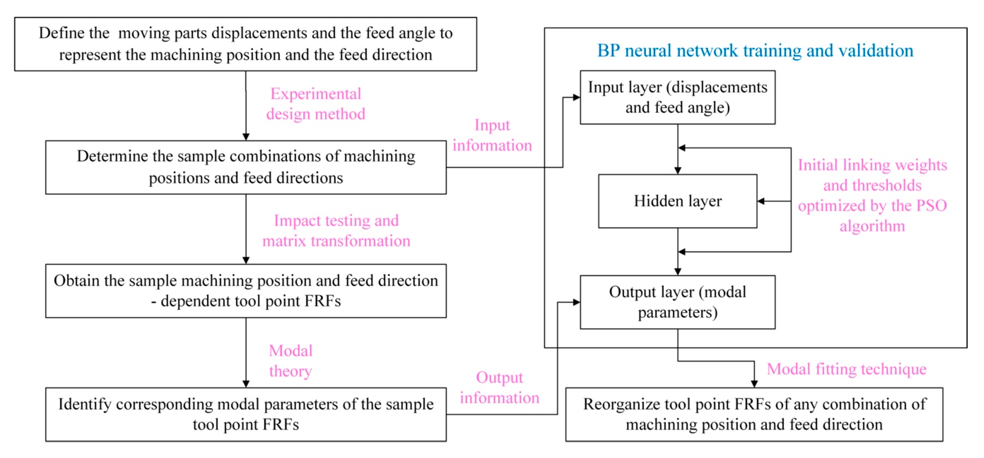
Figure 1. A flowchart for describing the whole research.
Symmetry 12 01073 g001
Figure 2. (a) Comparisons between the original and fitted FRFs; (b) The machine tool and feed direction coordinate system.
Symmetry 12 01073 g002
Figure 3. (a) A two DOF dynamic model of milling process; (b) Structure of a BP neural network with three layers.
Symmetry 12 01073 g003
Figure 4. Flow chart of the PSO-BP neural network.
Symmetry 12 01073 g004
Figure 5. The studied machine tool and the impact testing information.
Symmetry 12 01073 g005
Figure 6. (a) Tool point FRFs in different u directions; (b) Tool point FRFs in different v directions.
Symmetry 12 01073 g006
Figure 7. (a) An example tool point FRF in v direction and the identified 3 modes; (b) Comparisons of the predicted and measured FRFs of u and v directions at one position.
Symmetry 12 01073 g007
Figure 8. The feed direction-dependent limiting axial cutting depths for different machining positions. (a) aplim_feed values for three positions along x direction; (b) aplim_feed values for three positions along y direction; (c) aplim_feed values for three positions along z direction.
Symmetry 12 01073 g008
Table 1. The factors and their levels for designing the orthogonal experiment.
FactorsLevels
12345678
x/mm70140210280350420490550
y/mm50100150200250300350400
z/mm50100150200250300350400
θ22.54567.590112.5135157.5180
n/rpm200040006000800010,00012,00014,00015,000
Table 2. 64 orthogonal experiment schemes for obtaining the tool point FRFs and analyzing the machining stability.
No.xyzθnaplim-feed/mmNo.xyzθnaplim-feed/mm
1746377.5333122224.74
2386457.2734551234.14
3717267.4835342812.57
4652468.0236827344.80
5331721.6537616822.33
64416823.338287611.53
7573411.7739485246.95
8537857.2940133331.87
94325710.7411666615.1
10278521.5342234167.64
11467421.6843836215.83
12221478.8044818431.37
13414757.1245368277.17
14661356.9446144444.02
15872658.9247764511.55
16313543.8748845125.14
17854876.98495156712.75
18423866.8050476134.66
19753621.4951256743.97
20357189.2352735487.74
21647531.2153324631.19
22243259.6354638644.10
23548768.0555674288.87
24863787.1356728159.90
255265813.91571555510.08
26771844.8858584322.26
27458312.4959188886.11
28265831.9360212389.33
298815612.661683176.64
30625711.7862375367.24
31562146.6963177776.76
32111116.6064782731.35
Table 3. Identified modal parameters of one sample tool point FRF.
Mode No.123
Natural frequency ω (Hz)3846361428
Modal damping ratio ζ (%)4.175.354.20
Modal stiffness K (×109 N/m)2.020.111.23
Table 4. Comparisons between the measured and predicted modal parameters for the second mode in u direction for the six testing samples.
Sample No.Natural Frequency ω (Hz)Modal Damping Ratio ζ (%)Modal Stiffness K (×109 N/m)
MeasuredPredictedError (%)MeasuredPredictedError (%)MeasuredPredictedError (%)
1122812310.243.743.760.533.963.990.76
2123612320.323.563.652.522.622.543.05
3123212330.083.573.531.121.051.031.90
4124012340.483.713.690.542.372.283.79
5123612330.243.723.642.157.077.080.14
6122012210.083.443.323.480.8440.8500.71
Table 5. Results of range analysis and variance analysis according to the orthogonal experiment.
x/mmy/mmz/mmθn/rpmx/mm
Range analysisK155.2350.8468.8456.4924.12
K244.3551.9152.3454.8020.82
K340.2046.8439.2042.4617.71
K463.6661.3939.6340.6639.29
K556.8546.4153.6055.4667.14
K639.8848.1460.5468.2972.88
K741.9244.6239.9837.8167.32
K852.7544.7040.7138.8885.56
Range R23.4716.7729.6530.4867.85
Optimal levelsx4y4z1θ6n8
Variance analysisSSj70.1026.77111.52105.29632.10
Freedom dfj77777
Variance Sj10.013.8215.9315.0490.30
F value3.371.295.355.0630.35
Standard Fα value2.3592.3592.3592.3592.359