Article

Intuitionistic Fuzzy Three-Way Decision Model Based on the Three-Way Granular Computing Method

College of Artificial Intelligence, Beijing Normal University, Beijing 100875, China
*
Author to whom correspondence should be addressed.
Symmetry 2020, 12(7), 1068; https://doi.org/10.3390/sym12071068
Submission received: 3 June 2020 / Revised: 23 June 2020 / Accepted: 27 June 2020 / Published: 29 June 2020

Abstract

:
Three-way decisions, as a general model for uncertain information processing and decisions, mainly utilize the threshold generated by the decision cost matrix to determine the decision category of the object. However, the determination of the threshold is usually accompanied by varying degrees of subjectivity. In addition, the potential symmetrical relationship between the advantages and disadvantages of the decision cost is also a problem worthy of attention. In this study, we propose a novel intuitionistic fuzzy three-way decision (IFTWD) model based on a three-way granular computing method. First, we present the calculation methods for the possibility of membership state and non-membership state, as well as prove the related properties. Furthermore, we investigate the object information granules, i.e., the fine-grained, medium-grained, and coarse-grained objects, by combining the state probability distribution and probability distribution. Then, for decision and evaluation issues, we define the superiority-compatibility relation and inferiority-compatibility relation for IFTWD model construction. In addition, we use the superiority degree and inferiority degree instead of the original thresholds and design a new method for evaluating decision cost. Finally, we focus on the algorithm research of the proposed model and present an empirical study of agricultural ecological investment in Hubei Province to demonstrate the effectiveness of our model.

1. Introduction

Pawlak proposed the rough set theory [1], which rapidly attracted the attention of scholars and was successfully applied to machine learning [2,3], formal concept analysis [4,5,6], knowledge engineering [7,8], granular computing [9,10], etc. The rough set mainly utilizes the equivalence relation to express the classification ability of domain knowledge. In detail, the domain of discourse is divided into three disjoint subsets according to the upper and lower approximations, i.e., the positive domain, the negative domain, and the boundary domain [11]. However, such strict equivalence relations will easily cause excessive noise and redundant information in the boundary domain. From the perspective of improving the fault tolerance of the boundary, scholars have introduced various improved rough set models [12,13,14,15,16].
In particular, based on the decision-theoretic rough sets (DTRS) model [13], Yao proposed the three-way decision theory [17,18], which provided a reasonable semantic interpretation for the positive, boundary, and negative domains of the rough set. In simple terms, corresponding to these three domains, different strategies are adopted, i.e., acceptance, non-commitment, and rejection [19]. As a more general decision model and information-processing mode, three-way decision theory has received extensive attention from scholars since it was proposed. To date, the research on three-way decisions can be categorized into the following two aspects, namely, modelling and application. In terms of model construction, the traditional method is to study three-way decisions by constructing different DTRS models (such as studying the conditional probability and loss functions in DTRS) [20,21,22,23,24,25,26,27,28,29,30,31,32]. For example, to solve the problem that the traditional DTRS model cannot deal with the multi-valued set loss function, Zhao et al. [21] generalized DTRS models and investigated three-way decisions. Liang [23,24] introduced dual hesitant fuzzy sets and intuitionistic fuzzy point operators into DTRS and systematically researched the corresponding three-way decision models. In addition, experimental data in real life are not always clear and definite, and the three-way decision model should have the ability to handle uncertain and fuzzy information. Under the guidance of such ideas, the fuzzy three-way decision model [20], intuitionistic fuzzy three-way decision model [22,25], and three-way decision model of incomplete information systems [26,27] have successively been presented. Furthermore, interdisciplinary research has offered a possible way to separate the three-way decisions from the DTRS framework and form a set of independent ideological and theoretical systems. For instance, Zhang et al. [28] focused on the inclusion measures of characterizing interval sets and discussed the construction of a three-way decision model. Wang et al. [29] incorporated the psychological attitude of the decision maker into the decision-making process and constructed a three-way decision model based on cumulative prospect theory. Yang et al. [30] combined granular computing and investigated a sequential three-way decision model for multi-classification. Qi et al. [31] and Yu et al. [32] explored the relationship between three-way concept lattices and three-way decisions from the perspective of formal concept analysis. The research on the application of three-way decision theory mainly focuses on three-way clustering [33,34], three-way classification [35,36], three-way attribute reduction [37,38,39], three-way uncertainty decision [25,40,41], and three-way conflict analysis [42,43]. For instance, Xu et al. [35] focused on the semantics of three-way decisions from the perspective of a confusion matrix and investigated related clustering methods. Considering the clustering problem of high-dimensional multi-view data, Yu et al. [33] presented a three-way clustering method. By introducing the concepts of cost-sensitive and monotonic result-cost, Ma et al. [37] studied three-way attribute reduction in the two dimensions of result-cost and test-cost sensitivity. The above studies have all contributed to the development of the three-way decision theory.
The concept of granular computing was originally proposed by Zadeh [44], and it is regarded as a powerful tool for knowledge discovery and dealing with uncertain problems. Subsequently, Yao systematically investigated the framework of granular computing and presented a triarchic theory, i.e., a granular structure should include the three aspects of granularity, layer, and hierarchical structure [45,46]. Over the last several years, scholars have carried out a series of studies on granular computing. Leng et al. [47] combined granular computing and deep learning to improve the quality and efficiency of service planning when learning imbalanced data. Based on granular computing, Loia et al. [48] provided a method of constructing a time-dependent view. Lu et al. [49] adopted the idea of granular computing and studied a language model with high precision and interpretability. Yu et al. [50] incorporated the granularity of information into the decision process and discussed a granular-driven three-way decision model. Most strikingly, Yao [51] introduced the idea of three-way decisions into granular computing and proposed the three-way granular computing model, as well as gave a framework of trisecting-acting-outcome (TAO). In light of the TAO model, we mainly need to solve the following three tasks [51]: (1) divide the whole into three parts (trisecting), (2) take appropriate strategies for each of the three parts (acting), and (3) evaluate the effectiveness of the results of the first two steps (outcome). References [52,53] further elaborate the TAO model in detail and explain the concept of tri-level thinking. These studies have enriched the connotation of granular computing and provided excellent ideas and orientations for its development.
However, to the best of our knowledge, the existing work has rarely utilized the idea of three-way granular computing to study the IFTWD model. In addition, there is a lack of objective evaluation methods for the results of IFTWD. Fortunately, the framework of the TAO model enables us to address the above two problems in a flexible way. Since the TAO model is just a bare framework, it is necessary to analyse the specific problem and give concrete interpretations of trisection, strategies, and outcome [53]. Therefore, information granulation, decision stratification, and evaluation subdivision are carried out on the domain objects to achieve the materialization of the TAO model and to construct the IFTWD model. The main contributions of this paper are as follows.
(1)
The concepts of membership state possibility and non-membership state possibility are defined, and their related properties are proved. Then, according to the relationship between the state probability distribution and the probability distribution, we give an approximate division rule for the object information granularity.
(2)
By combining object information granules and dominance relation, we propose superiority-compatibility relation and inferiority-compatibility relation. Furthermore, we deduced the IFTWD model on the basis of the superiority-compatibility class and inferiority-compatibility class.
(3)
To objectively evaluate the decision-making results and analyze the potential symmetrical relationship between decision costs, we define the concepts of advantage cost and disadvantage cost, and create a secondary decision strategy for boundary domain objects.
As we stated above, the main purpose of this investigation is to construct an intuitionistic fuzzy three-way decision model through the three-way granular computing method. The rest of the structure of this paper is as follows. In Section 2, we simply review some basic knowledge of three-way decisions and intuitionistic fuzzy sets. In Section 3, we propose a method for calculating the object information granularity and then define the superiority-compatibility relation to construct the IFTWD model. Finally, a new strategy for analysing decision costs is given. In Section 4, the validity of the model proposed in this paper is verified by an example. In Section 5, the paper ends with conclusions.

2. Preliminaries

This section briefly reviews some basic concepts [1,13,17,18,41,54,55]. Throughout this paper, we assume that the domain of discourse U and attribute set A are both non-empty finite sets.

2.1. Pawlak Rough Set

Pawlak believes that knowledge can be divided by equivalence relations to form an easy-to-express formal language that helps people understand and calculate.
Definition 1.
[1] Let U be the universe of discourse; R is an equivalent relationship defined on U, and a p r = ( U , R ) is an approximate space. The division of the universe U under the equivalence relation R can be described as U / R = { [ x ] R | x U } , where [ x ] R is an equivalence class containing x. For any X U , its upper and lower approximate sets can be expressed as:
a p r ¯ R ( X ) = { x U | [ x ] R X } , a p r _ R ( X ) = { x U | [ x ] R X } .
It can be found that both the upper and lower approximations are crisp sets, and the elements in the upper approximation overlap with the equivalent classes, while the elements in the lower approximation are completely contained in the equivalent classes. Therefore, the discourse domain can be divided into three disjointed parts by upper and lower approximations, namely, the positive domain POS(X), the negative domain NEG(X), and the boundary domain BND(X) are as follows:
P O S ( X ) = a p r _ R ( X ) ,    N E G ( X ) = U a p r ¯ R ( X ) ,    B N D ( X ) = a p r ¯ R ( X ) a p r _ R ( X ) .

2.2. Three-Way Decision

Due to the strict equivalence relations, the positive and negative domains obtained by the Pawlak method are correct and meet the requirements, i.e., there is no wrong acceptance or rejection. Furthermore, in practice, the BND region often has too much redundant information. To overcome its shortcomings, Yao proposed three-way decision theories combined with DTRS and Bayesian minimum risk theory, which gave rough sets a new semantic interpretation.
Definition 2.
[13,17,18] Let Ω = { X , ¬ X } be a set representing two complementary states; i.e., element x belongs to object X or does not belong to object X. Γ = { a P , a B , a N } represents three different decisions, where a P is the acceptance decision, a B is the delay decision, and a N is the rejection decision. The decision losses caused by actions taken in different states are shown in Table 1.
In Table 1, λ P P , λ B P , and λ N P represent the cost losses of adopting a P , a B , and a N decisions when in state X. Similarly, λ P N , λ B N , and λ N N denote the decision loss under state ¬ X . Therefore, the expected loss of object x under different actions is R ( a i | [ x ] ) ( i = P , B , N ) , which can be expressed as follows:
R ( a P | [ x ] R ) = λ P P Pr ( X | [ x ] R ) + λ P N Pr ( ¬ X | [ x ] R ) , R ( a B | [ x ] R ) = λ B P Pr ( X | [ x ] R ) + λ B N Pr ( ¬ X | [ x ] R ) , R ( a N | [ x ] R ) = λ N P Pr ( X | [ x ] R ) + λ N N Pr ( ¬ X | [ x ] R ) .
where Pr ( X | [ x ] R ) and Pr ( ¬ X | [ x ] R ) represent the probabilities that the equivalence class belongs to X and ¬ X .
According to the Bayesian minimum risk decision process, we can obtain the following decision rules:
( P 1 ) If R ( a P | [ x ] R ) R ( a B | [ x ] R ) and R ( a P | [ x ] R ) R ( a N | [ x ] R ) , then x P O S ( X ) , ( N 1 ) If R ( a N | [ x ] R ) R ( a P | [ x ] R ) and R ( a N | [ x ] R ) R ( a B | [ x ] R ) , then x N E G ( X ) , ( B 1 ) If R ( a B | [ x ] R ) R ( a P | [ x ] R ) and R ( a B | [ x ] R ) R ( a N | [ x ] R ) , then x B N D ( X ) .
By a reasonable hypothesis, λ P P λ B P < λ N P and λ N N λ B N < λ P N ; if the BND domain exists, then ( λ B P λ P P ) ( λ B P λ N N ) < ( λ P N λ B N ) ( λ N P λ B P ) , and condition Pr ( X | [ x ] R ) + Pr ( ¬ X | [ x ] R ) = 1 holds. Equation (4) can be simplified as:
( P ) If Pr ( X | [ x ] R ) α , then x P O S ( X ) , ( B ) If β < Pr ( X | [ x ] R ) < α , then x B N D ( X ) , ( N ) If Pr ( X | [ x ] R ) β , then x N E G ( X ) .
Here, α and β represent:
α = λ P N λ B N ( λ P N λ B N ) + ( λ B P λ P P ) , β = λ B P λ N N ( λ B P λ N N ) + ( λ N P λ B P ) .
Through the above analysis, we can find that the three-way decision rules are closely related to the ( α , β ) thresholds. In the uncertain environment, eliminating the constraints of DTRS and constructing decision evaluation methods from other perspectives is a topic worthy of further research.

2.3. Intuitionistic Fuzzy Set and Dominance Relation

Definition 3.
[54] Let U be the universe and S ˜ = { < x , μ S ˜ ( x ) , ν S ˜ ( x ) > | x U } be an intuitionistic fuzzy set on U, where μ S ˜ ( x ) : U [ 0 , 1 ] , ν S ˜ ( x ) : U [ 0 , 1 ] and 0 μ S ˜ ( x ) + ν S ˜ ( x ) 1 . μ S ˜ ( x ) and ν S ˜ ( x ) are the membership and non-membership degrees of object x, respectively, and η S ˜ ( x ) = 1 η S ˜ ( x ) ν S ˜ ( x ) ( 0 η S ˜ ( x ) 1 ) is called the hesitancy degree or intuitionistic fuzzy index. It is easy to find that when η S ˜ ( x ) = 0 , the intuitionistic fuzzy set degenerates into a fuzzy set. For convenience, S ˜ = { < x , μ S ˜ ( x ) , ν S ˜ ( x ) > | x U } is abbreviated as S ˜ = ( μ S ˜ ( x ) , ν S ˜ ( x ) ) , and all intuitionistic fuzzy sets on U are denoted as I F ( U ) .
Definition 4.
[54] Let U be the universe; B ˜ = { < x , μ B ˜ ( x ) , ν B ˜ ( x ) > | x U } and C ˜ = { < x , μ C ˜ ( x ) , ν C ˜ ( x ) > | x U } are two intuitionistic fuzzy sets on U. Then, the basic operation is as follows:
(1).
B ˜ = C ˜ { ( μ B ˜ ( x ) = μ C ˜ ( x ) ) ( ν B ˜ ( x ) = ν C ˜ ( x ) ) | x U }
(2).
B ˜ C ˜ { ( μ B ˜ ( x ) μ C ˜ ( x ) ) ( ν B ˜ ( x ) ν C ˜ ( x ) ) | x U }
(3).
B ˜ C ˜ = { ( x , { μ B ˜ ( x ) , μ C ˜ ( x ) } , { ν B ˜ ( x ) , ν C ˜ ( x ) } ) | x U }
(4).
B ˜ C ˜ = { ( x , { μ B ˜ ( x ) , μ C ˜ ( x ) } , { ν B ˜ ( x ) , ν C ˜ ( x ) } ) | x U }
(5).
B ˜ C = { ( x , ν B ˜ ( x ) , μ B ˜ ( x ) ) | x U }
Definition 5.
[41] Let P s : x [ 0 , 1 ] and N g : x [ 0 , 1 ] , C p : x [ 0 , 1 ] and C n : x [ 0 , 1 ] be two pair sets of functions. For A I F ( U ) , the following conditions are satisfied:
(1).
P s ( μ ( x ) ) = 1 , N g ( ν ( x ) ) = 0 .
(2).
P s ( U i U U i ( μ ( x ) ) ) = i n f U i U P s ( μ U i ( x ) ) , N g ( U i U U i ( ν ( x ) ) ) = s u p U i U N g ( ν U i ( x ) ) .
Then, ( P s , N g ) represents an intuitionistic fuzzy possibility measure on U.
Definition 6.
[55] Let quaternion Ψ = ( U , A , V , f ) represent an information system, where U = { x 1 , x 2 , , x n } is the universe, A = { B 1 , B 2 , , B m } is the attribute set, V is the value domain of attribute B j , and f : U × A V is an information mapping function. The superiority and inferiority relations are expressed as follows:
Superiority relation: R B = { ( x i , x j ) U × U : f ( x i , B ) f ( x j , B ) , B A } .
Inferiority relation: R B = { ( x i , x j ) U × U : f ( x i , B ) f ( x j , B ) , B A } .
For the convenience of description, if V B j I F ( U ) , we use Ψ ˜ = ( U , A , V ˜ , f ) to represent an intuitionistic fuzzy information system, abbreviated as Ψ ˜ .

3. IFTWD Derived from the Three-Way Granular Computing Method

The TAO model is a generalized framework for three-way granular computing. To enrich its connotation, we first construct object information granules by fusing state probability functions of uncertain information features to solve the trisecting problem. Second, for the problems of acting and outcome, the concept of a superiority-compatible relation is given, and the decision results are evaluated by the superiority degree and inferiority degree. Finally, the secondary decision is made on the objects in the boundary domain, and the IFTWD model decision rules and algorithms are derived.

3.1. State Possibility and Information Granularity

Reference [41] considers the composition of intuitionistic fuzzy probability measured from a macro perspective, but from a micro perspective, if the overlap of the membership degree of elements is not large or the conflict of non-membership degree is not strong, then the useful information of used elements cannot be integrated and utilized. If attribute B ˜ A has multiple states under object x i U , the possibility in a certain state is simply referred to as the state possibility.
Definition 7.
Let the triplet Θ = { U , A , S q } be a state possibility space, where U is the universe, A is the attribute set, and S p ( S q + ( x i ) , S q ( x i ) ) is the state possibility function established between U and A. Specifically, S q + and S q indicate the membership state possibility and non-membership state possibility, respectively. For any x i U , B ˜ , C ˜ A , satisfying the following conditions:
(M1) 0 < S q B ˜ + ( μ ( x i ) , ν ( x i ) ) 1 , 0 S q B ˜ ( μ ( x i ) , ν ( x i ) ) < 1 .
(M2) S q B ˜ + ( x i ) = 1 holds, if and only if μ B ˜ ( x i ) = 1 , ν B ˜ ( x i ) = 0 ; S q B ˜ ( x i ) = 1 holds, if and only if μ B ˜ ( x i ) = 0 , ν B ˜ ( x i ) = 1 .
(M3) B ˜ A , if μ B ˜ ( x i ) is given, S q B ˜ + ( x i ) is negatively correlated with ν B ˜ ( x i ) , and S q B ˜ ( x i ) is positively correlated with ν B ˜ ( x i ) .
Then, Sq is called the state possibility function. On the basis of (M1)–(M3), if Sq satisfies:
(M4) B ˜ , C ˜ A , if μ B ˜ ( x i ) , μ C ( x i ) 0.5 and μ B ˜ ( x i ) μ C ˜ ( x i ) + η C ˜ ( x i ) hold, S q B ˜ + ( x i ) > S q C ˜ + ( x i ) .
Then, Sq is called the weakened non-membership state possibility function. Similarly, if Sq satisfies:
(M5) B ˜ , C ˜ A , if ν B ˜ ( x i ) , ν C ( x i ) 0.5 and ν B ˜ ( x i ) + η B ˜ ( x i ) ν C ˜ ( x i ) hold, S q B ˜ ( x i ) < S q C ˜ ( x i ) .
Then, Sq is called the enhanced membership state possibility function.
(M1) indicates that the state probability of any object is between 0 and 1. In addition, since probability only describes the difficulty of an event, (M2) gives the extreme value condition of state possibility, and (M3) is the monotonic condition of state possibility. Moreover, it is easy to determine that the membership range of the state possibility is between [ μ ( x i ) , μ ( x i ) + η ( x i ) ] and that the non-membership state possibility is between [ ν ( x i ) , ν ( x i ) + η ( x i ) ] , so (M4) and (M5) can be regarded as the weakening and strengthening conditions of the state possibility.
Theorem 1.
S p ( S q B ˜ + ( x i ) , S q B ˜ ( x i ) ) is the state possibility function of attribute B ˜ under object x i . For any B ˜ A , Sq can be expressed as:
S p = { S p B ˜ + ( x i ) = 1 + π 5 ln max { 1 ν B ˜ ( x i ) , η B ˜ ( x i ) + ν B ˜ ( x i ) } exp ( η B ˜ ( x i ) + ν B ˜ ( x i ) ) S p B ˜ ( x i ) = ln ( min { 1 μ B ˜ ( x i ) , η B ˜ ( x i ) + μ B ˜ ( x i ) } exp ( η B ˜ ( x i ) + μ B ˜ ( x i ) ) + 1 )
Proof. 
(M2) is easily proven by formula (7), and only (M1) and (M3) are proven below.
(M1) By Definition 3, B ˜ A , max { 1 ν B ˜ ( x i ) , η B ˜ ( x i ) + ν B ˜ ( x i ) } max { η B ˜ ( x i ) + μ B ˜ ( x i ) , η B ˜ ( x i ) + ν B ˜ ( x i ) } , i.e., max { μ B ˜ ( x i ) , ν B ˜ ( x i ) } . The following will take max = μ B ˜ ( x i ) as an example to prove. Since μ B ˜ ( x i ) + ν B ˜ ( x i ) [ 0 , 1 ] is a fixed value, we can obtain 0.5 max 1 and exp ( μ B ˜ ( x i ) + ν B ˜ ( x i ) ) 1 . Let ο B ˜ = ln μ B ˜ ( x i ) / exp ( μ B ˜ ( x i ) + ν B ˜ ( x i ) ) 0 ; when μ B ˜ ( x i ) = 1 , ο B ˜ reaches a maximum of 0, and when μ B ˜ = ν B ˜ = 0.5 , ο B ˜ reaches a minimum of 0.3. Therefore, we can obtain 0 < p B ˜ + ( x i ) 1 . Similarly, 0 S p B ˜ ( x i ) < 1 holds.
(M3) B ˜ A , when μ B ˜ ( x i ) is given and ν B ˜ ( x i ) increases, the following two cases exist.
Case 1: Since ο B ˜ is a decreasing function with respect to ν B ˜ ( x i ) , S p B ˜ + ( x i ) will decrease as ν B ˜ ( x i ) increases; i.e., they have a negative correlation.
Case 2: Let κ B ˜ = min { 1 μ B ˜ ( x i ) , η B ˜ ( x i ) + μ B ˜ ( x i ) } / exp ( μ B ˜ ( x i ) + ν B ˜ ( x i ) ) ; it is easy to determine that κ B ˜ and ν B ˜ ( x i ) change in the same direction, and the logarithmic function with e as the base monotonically increases in the domain, which leads to a positive correlation between ν B ˜ ( x i ) and ln ( ε B ˜ + 1 ) .
In summary, S p ( S q B ˜ + ( x i ) , S q B ˜ ( x i ) ) is the state possibility function.  □
Remark. 
Equation (7) considers the effects of the degree of hesitation converted into the membership state possibility and the non-membership state possibility. On the one hand, the degree of membership and non-membership represent deterministic information to a certain extent. On the other hand, due to the existence of unknown information, the degree of hesitation has the arbitrary possibility of turning into membership and non-membership. Therefore, the following points need to be considered in actual calculations:
(1)
Satisfy the weak and strong conditions of (M4) and (M5). Specifically, there is always a possibility that (1,0) satisfies the enhanced membership state and (0,1) satisfies the weakened non-membership state.
(2)
The following two state values need special consideration to make the calculation results meaningful.
Case 1: when the state value is (1,0), we only need to consider the membership state possibility.
Case 2: when the state value is (0,1), we only need to consider the non-membership state possibility.
(3)
When the state value is ( 0 , 0 ) , the conversion of hesitation degree is completely uncertain. Relative to the determined membership and non-membership degrees, the intuitionistic fuzzy index is caused by the existence of a variety of unknown information. For the sake of analysis, it is assumed that these unknown factors are independent. According to the central limit theorem, these independent unknown factors obey the Gaussian distribution (hypothetical standard Gaussian distribution), and then the transformation degree of the intuitionistic fuzzy index can be expressed as follows:
S p η ( x i ) = 1 2 π exp ( ( η ( x i ) ) 2 2 )
Lemma 1.
(1) B ˜ A , if μ B ˜ ( x 1 ) = μ B ˜ ( x 2 ) and ν B ˜ ( x 1 ) ν B ˜ ( x 2 ) , then S q B ˜ + ( x 1 ) S q B ˜ + ( x 2 )
(2) B ˜ A , if ν B ˜ ( x 1 ) = ν B ˜ ( x 2 ) and μ B ˜ ( x 1 ) μ B ˜ ( x 2 ) , then S q B ˜ ( x 1 ) S q B ˜ ( x 2 ) .
(3) B ˜ A , x i U , 0 S q B ˜ + ( x i ) + S q B ˜ ( x i ) 1 .
Proof. 
It is straightforward to prove Lemma 1 by use of Definition 7 and Theorem 1. □
Lemma 2.
B ˜ A , when μ B ˜ ( x i ) = 0 , the change in ν B ˜ ( x i ) will not cause a change in the S q B ˜ + ( x i ) value.
Proof. 
When μ B ˜ ( x i ) = 0 , the possibility of a membership state is completely determined by the hesitation degree, and the amount of membership information contained in the hesitation degree is uncertain. According to Equation (7), ν B ˜ ( x i ) + π B ˜ ( x i ) is a certain value regardless of how ν B ˜ ( x i ) changes. Therefore, a change in ν B ˜ ( x i ) does not cause a change in the value of S q B ˜ + ( x i ) . Analogically, we can obtain that when ν B ˜ ( x i ) = 0 , the change in μ B ˜ ( x i ) will not cause the value of S q B ˜ ( x i ) to change. □
Example 1.
Reference [56] calculated the risk levels of different audit objects in the intuitionistic fuzzy security audit evaluation system, where the universe is U = { x 1 , x 2 , x 3 , x 4 } and the attribute set is A = { B ˜ , C ˜ , D ˜ , E ˜ , F ˜ , G ˜ } , as shown in Table 2.
According to Theorem 1, we can obtain the membership state possibility and non-membership state possibility of each object under attribute set A, as shown in Figure 1. Example 1 demonstrates that the higher the possibility of the membership state of the object x i under the attribute B ˜ A is, the lower the possibility of the corresponding non-membership state. In addition, the membership state probability and the non-membership state possibility are given based on the maximum transformation condition of hesitation degree, which can only be quantitatively analysed from the degree of difficulty of a certain state. Therefore, the similarity or consistency between the probability distribution and the state probability distribution needs further analysis.
Definition 8.
Let quaternion Λ = { U , A , S p , P } be a state probability-probability space, where U is the universe of discourse, A is the attribute set, S p is the state probability function built between U and A, and P is the probability conversion function. x i U , B ˜ A , if the state value ( μ B ˜ ( x i ) , ν B ˜ ( x i ) ) of the object x i with respect to the attribute B ˜ is regarded as a two-dimensional random variable about the membership function and the non-membership function, then the relationship between the probability distribution and the state probability distribution is shown in Table 3.
P k = max { B ˜ A μ B ˜ ( x i ) μ + ν ν B ˜ ( x i ) μ + ν } , μ = max { μ B ˜ ( x i ) S q B ˜ + ( x i ) } , ν = min { ν B ˜ ( x i ) + S q B ˜ ( x i ) ν B ˜ ( x i ) S q B ˜ ( x i ) } , k = 1 , 2 , , 9 . If the value is (0,0), let P k ( 0 , 0 ) = 0 .
Definition 9.
Let ψ ˜ = ( U , A , V ˜ , f ) be an intuitionistic fuzzy information system. For any x i U , B ˜ j A , there is a state value ( μ B ˜ ( x i j ) , ν B ˜ ( x i j ) ) corresponding to f, and the matrix form is M = ( μ B ˜ ( x i j ) , ν B ˜ ( x i j ) ) n × m = ( x i j ) n × m . The expression ability of object x i in the complete set A, i.e., the information granularity G, can be expressed as follows:
{ θ η = x i U B ˜ j A P k ( min { S p η ( x i j ) } ) log 2 ( P k ( min { S p η ( x i j ) } ) ) G ( x i j ) = | min { x i U B ˜ j A S B ˜ + ( x i j ) } min { x i U B ˜ j A S B ˜ ( x i j ) } |
S B ˜ + ( x i j ) = ( S p B ˜ + ( x i j ) + θ η ) log 2 ( ( S p B ˜ + ( x i j ) + θ η ) / P k ( x i j ) ) } , S B ˜ ( x i j ) = ( S p B ˜ ( x i j ) + θ η ) log 2 ( ( S p B ˜ ( x i j ) + θ η ) / P k ( x i j ) ) } . If there is consistently more than one S p η ( x i j ) , the mean value is taken as the final result. In Equation (9), θ η ensures that the information uncertainty when the state probability is converted into a probability value remains unchanged, and G ( x i j ) provides the degree of fitting between the state probability and probability distributions after adding uncertain information, i.e., the smaller the information granularity G of an object is, the stronger its expressive power. Since probability is generally understood as the difficulty of an event, probability is understood as the frequency of an event. In the intuitionistic fuzzy system ψ ˜ , a high probability of a certain state means that it has a high probability of occurrence. Conversely, a low probability of a certain state implies that it has a low probability of occurrence. Therefore, the assumptions without loss of generality are P b i g ( x i ) S q b i g ( x i ) , S q s m a l l ( x i ) P s m a l l ( x i ) .
Combining Table 2 and Equation (9), we can obtain the approximate division of object information granularity, as shown in Table 4.
“O” and “ × ” indicate that the conditions are satisfied and not satisfied, respectively. The approximate division rules for the granularity of object information obtained from Table 4 are as follows:
(1).
If C 1 and C 2 , then x i G F .
(2).
If C 1 and ¬ C 2 , or ¬ C 1 and C 2 , then x i G M .
(3).
If ¬ C 1 and ¬ C 2 , then x i G C .
It is worth noting that the conditions C 1 and C 2 are just a trend judgement. In practice, we also need to perform quantitative analysis and calculation. In addition, to increase the noise tolerance of the C 1 and C 2 conditions, the Euclidean distance of the state probability and probability value is used as the elasticity judgement interval, which is expressed as follows:
{ D ( S q B ˜ + ( x i ) , P k ( x i ) ) = | ( S q max + ( x i ) P k ( x i ) ) 2 ( S q η ( x i ) P k ( x i ) ) 2 | D ( S q B ˜ ( x i ) , P k ( x i ) ) = ( S q min ( x i ) P k ( x i ) ) 2 + ( S q η ( x i ) P k ( x i ) ) 2
S q max + ( x i ) represents the maximum membership state possibility of object x i under attribute set A. Due to the existence of uncertain information, the difference between the Euclidean distance of S q max + ( x i ) , S q η ( x i ) and P k ( x i ) is used as the lower bound of the judgment condition P b i g ( x i ) S q b i g ( x i ) . Similarly, the sum of Euclidean distance between the S q min ( x i ) , S q η ( x i ) , and P k ( x i ) is used as the upper bound as the judgment condition S q s m a l l ( x i ) P s m a l l ( x i ) . Thus, the approximate division conditions C 1 and C 2 in Table 4 can be adjusted as:
C 1 * : P b i g ( x i ) S q b i g ( x i ) [ 0 , D ( S q max + ( x i ) , P k ( x i ) ) C 2 * : S q s m a l l ( x i ) P s m a l l ( x i ) [ 0 , D ( S q min ( x i ) , P k ( x i ) )
Example 2.
According to the relationship between the state probability distribution and the probability distribution as well as the division conditions, the information granularity of each object in Table 3 can be calculated as shown in Table 5.
The granular classification algorithm of the universe object is given below. First, the membership state possibility and non-membership state possibility of the universe object x i under attribute set A are calculated. Then, according to the relationship between the state probability distribution and the probability distribution, the information granularity value of object x i is obtained. Finally, according to the C 1 * and C 2 * judgement conditions, the information granularity of the universe object is approximately classified.
Algorithm 1 Granularity classification of objects in the universe of discourse
1: Input S = ( U , A , V ˜ , f ) , Λ = ( U , A , S p , P ) , x i U , B ˜ A
2: Initialization (1) parameters: μ = max { μ B ˜ ( x i ) S q B ˜ + ( x i ) } , ν = min { ν B ˜ ( x i ) + S q B ˜ ( x i ) ν B ˜ ( x i ) S q B ˜ ( x i ) }
3: functions: (1) S B ˜ + ( x i j ) = ( S p B ˜ + ( x i j ) + θ η ) log 2 ( ( S p B ˜ + ( x i j ) + θ η ) / P k ( x i j ) ) }
4: (2) S B ˜ ( x i j ) = ( S p B ˜ ( x i j ) + θ η ) log 2 ( ( S p B ˜ ( x i j ) + θ η ) / P k ( x i j ) ) }
5: (3) P k = max { B ˜ A μ B ˜ ( x i ) μ + ν ν B ˜ ( x i ) μ + ν }
6: Output Granularity category of each object.
7: BEGIN
8: for Calculate the possibility of membership status and non-membership status do
9:     S p B ˜ + ( x i ) = 1 + π 5 ln max { 1 ν B ˜ ( x i ) , η B ˜ ( x i ) + ν B ˜ ( x i ) } exp ( η B ˜ ( x i ) + ν B ˜ ( x i ) ) ,
S p B ˜ ( x i ) = ln ( min { 1 μ B ˜ ( x i ) , η B ˜ ( x i ) + μ B ˜ ( x i ) } exp ( η B ˜ ( x i ) + μ B ˜ ( x i ) ) + 1 )
10:     if ( μ B ˜ ( x i ) , ν B ˜ ( x i ) ) = ( 0 , 0 ) then
11:       S p η ( x i ) = 1 2 π exp ( ( η ( x i ) ) 2 2 ) . // maximum hesitation probability state value
12:    end if
13: end for
14: for Calculate the information granularity of each object do
15:      θ η = x i U B ˜ j A P k ( min { S p η ( x i j ) } ) log 2 ( P k ( min { S p η ( x i j ) } ) ) // Get the hesitation factor impact
16:    then G ( x i j ) = | min { x i U B ˜ j A S B ˜ + ( x i j ) } min { x i U B ˜ j A S B ˜ ( x i j ) } | // Get the granularity value
17:    while Calculate the relationship between the granularity value C 1 * and C 2 * do
18:          C 1 * [ 0 , D ( S q max + ( x i ) , P k ( x i ) ) , C 2 * [ 0 , D ( S q min ( x i ) , P k ( x i ) )
19:         if G ( x i ) C 1 * C 2 * then
20:             Object x i is Fine-grained: x i G F // satisfies both C 1 * and C 2 *
21:             if G ( x i ) C 1 * C 2 * then
22:              Object x i is Medium-grained: x i G M // satisfies either C 1 * or C 2 *
23:            else
24:              Object x i is Coarse-grained: x i G C // satisfies neither C 1 * nor C 2 *
25:           end if
26:        end if
27:     end while
28: end for
29: END BEGIN

3.2. Superiority-Compatibility Relation and Decision Evaluation

According to the view of three-way granular computing [51,52,53], decision and evaluation are another focus after trisecting work. Therefore, in this section, the concept of the superiority-compatibility relation and the calculation method of the superiority degree are given. Accordingly, a new decision cost evaluation strategy is proposed, and the secondary decision is made for the BND domain objects.
Definition 10.
Let Ψ ˜ = ( U , A , V ˜ , f ) be an intuitionistic fuzzy information system; then, R δ is called the superiority-compatibility relation if and only if the following condition is satisfied:
R δ = { ( x i , x j ) U × U : ( G ( x i , B ˜ ) G ( x j , B ˜ ) ) ( | [ x i ] R | | [ x j ] R | ) }
Analogously, inferiority-compatibility R ε is as follows:
R ε = { ( x i , x j ) U × U : ( G ( x i , B ˜ ) G ( x j , B ˜ ) ) ( | [ x i ] R | | [ x j ] R | ) }
Equations (12) and (13) use the superiority-compatibility relation and inferiority-compatibility relation to replace the traditional equivalence relation, and | | [ x i ] R | and | [ x i ] R | represent the number of elements in the maximum superiority-compatibility class and the maximum inferiority-compatibility class of object x i , respectively. Moreover, R is defined as an object with a membership degree that is not greater than δ = min { x i U B ˜ A { max { μ B ˜ ( x i ) , μ B ˜ ( x j ) } } , and R is defined as an object with a membership degree that is not less than ε = max { x i U B ˜ A { min { ν B ˜ ( x i ) , ν B ˜ ( x j ) } } .
Thus, the superiority-compatibility class and inferiority-compatibility class are as follows:
[ x i ] R δ = { x j U | ( x i , x j ) x i R δ x j } = { x j U : ( G ( x i , B ˜ ) G ( x j , B ˜ ) ) ( | [ x i ] R | | [ x j ] R | ) } , [ x i ] R ε = { x j U | ( x i , x j ) x i R ε x j } = { x j U : ( G ( x i , B ˜ ) G ( x j , B ˜ ) ) ( | [ x i ] R | | [ x j ] R | ) } .
Theorem 2.
(1) .
If [ x 1 ] R δ , [ x 2 ] R δ , , [ x n ] R δ are superiority-compatibility classes on ψ ˜ , then [ x l ] R δ ( 1 l n ) makes [ x l ] R δ [ x max ] R δ hold, where [ x max ] R δ represents the largest superiority-compatibility classes.
(2) .
If [ x 1 ] R ε , [ x 2 ] R ε , , [ x n ] R ε are inferiority-compatibility classes on ψ ˜ , then [ x t ] R ε ( 1 t n ) makes [ x t ] R ε [ x max ] R ε hold, where [ x max ] R ε represents the largest inferiority-compatibility classes.
Proof. 
Since the methods are similar, only (1) is demonstrated below.
(1) Let L = { { [ x 1 ] R δ } , { [ x 2 ] R δ } , , { [ x n ] R δ } } and [ x 1 ] R δ [ x 2 ] R δ [ x n ] R δ , there must be [ x 2 ] R δ = [ x 1 ] R δ { x o } such that x o superiority-compatibility with all elements in [ x 1 ] R δ . By analogy, we can obtain that [ x l ] R δ ( 1 l n ) makes [ x l ] R δ [ x max ] R δ hold.
From Equations (12)–(14), it is easy to find that the superiority-compatibility relation introduces the dominance relation in the information granularity of the object and integrates the compatibility relation of the attribute set. Therefore, X U , the superiority lower approximation R _ ( X ) and inferiority upper approximation R ¯ ( X ) can be obtained as follows:
R _ ( X ) = { x i X , [ x i ] R δ ϕ [ x i ] R ε = ϕ } , R ¯ ( X ) = { x i X , [ x i ] R δ = ϕ [ x i ] R ε ϕ } ,
It can be seen that the lower approximation R _ ( X ) is a further conditional restriction on fine-grained objects and that the upper approximation R ¯ ( X ) is a stronger judgement condition on coarse-grained objects. □
Theorem 3.
X , Y U , we have the following conclusions:
(1).
R _ ( ϕ ) = ϕ , R ¯ ( ϕ ) = ϕ .
(2).
R ¯ ( R _ ( X ) ) = ϕ , R _ ( R ¯ ( X ) ) = ϕ .
(3).
R _ ( X Y ) = R _ ( X ) R _ ( Y ) , R _ ( X ) R _ ( Y ) R _ ( X Y ) .
(4).
R ¯ ( X Y ) = R ¯ ( X ) R ¯ ( Y ) , R ¯ ( X Y ) R ¯ X ) R ¯ ( Y ) .
(5).
X Y R _ ( X ) R _ ( Y ) .
Proof. 
It is straightforward to prove Theorem 1 by use of Definition 10. □
Theorem 4.
The elements that appear most frequently in the intersection of the superiority-compatible class and the inferiority–compatible class belong to the POS domain and the NEG domain, respectively, which can be formally expressed as | [ x i ] R ε | max R _ ( U ) , | [ x i ] R δ | max R ¯ ( U ) .
Proof. 
Suppose x i P O S , according to formula (14), we can obtain [ x i ] R ε = ϕ and [ x i ] R δ ϕ . On the one hand, if x j U ( i j ) , x j is necessarily inferior-compatible with x i , i.e., x i [ x j ] R ε , x j U , i j x i [ x j ] R ε , so the assumption holds. Similarly, if x i N E G , for any x j U ( i j ) , we have x i [ x j ] R δ and x j U , i j x i [ x i ] R δ , i.e., | [ x i ] R δ | max R ¯ ( U ) .
Based on further analysis, for any X U , the lower approximate set expression ability is strong and has full advantages, while the upper approximate set expression ability is weak and completely at a disadvantage. Therefore, the POS(X) domain, BND(X) domain and NEG(X) domain can be obtained as follows:
P O S ( X ) = R _ ( X ) N E G ( X ) = R ¯ ( X ) , B N D ( X ) = U R _ ( X ) R ¯ ( X )
Corresponding to Equation (16), the division rules of the POS domain, NEG domain, and BND domain can be expressed as follows:
( P 2 ) P O S = R _ ( X ) = { x i U | [ x i ] R δ ϕ [ x i ] R ε = ϕ } ( N 2 ) N E G = R ¯ ( X ) = { x i U | [ x i ] R δ = ϕ D [ x i ] R ε ϕ } ( B 2 ) B N D = U R _ ( X ) R ¯ ( X ) = ( P O S N E G ) C
Example 3.
Combined with the granularity information obtained in Example 2, the calculation of the superiority-compatibility class, the inferiority-compatibility class, the upper approximation set, the lower approximation set, and the classification result of each object is shown in Table 6.
From Example 3, on the one hand, from the perspective of object information granularity, the partition results obtained from R δ and R ε are related to the original granularity of the object to a certain extent. For example, x 1 G F , and the final decision result is x 1 P O S . On the other hand, due to the characteristics of R δ and R ε , there is generally only one object in the POS domain and NEG domain, which is quite different from the classical three-way decision division rules. In this way, although the correctness of the POS domain and NEG domain is guaranteed, there will be too many delayed decision objects in the BND domain, so it is particularly important to make circular decisions on the BND domain objects. Moreover, in the three-way granular computing method, apart from the trisecting and decision, evaluation also plays an important role. To solve the above problems and evaluate the decision results reasonably and objectively, the following will analyse the decision result through the advantage cost and disadvantage cost of the object.
Definition 11.
Let G ς ( x i ) ( ς { F , M , C } ) be the granularity information, and [ x i ] R δ is the superiority-compatibility class; then, the advantage cost ħ ( x i ) of object x i is as follows:
ħ ( x i ) = ln ( G ( x i ) ) exp ( x i | i = 1 n [ x i ] R δ [ x j ] R δ | | j = 1 n [ x i ] R δ [ x j ] R δ | , i j , x j U )
Correspondingly, the disadvantage cost of object x i is as follows:
ƛ ( x i ) = ln ( G ( x i ) ) exp ( x i | i = 1 n [ x i ] R ε [ x j ] R ε | | j = 1 n [ x i ] R ε [ x j ] R ε | , i j , x j U )
where | | represents the cardinality of the set. It can be known that the coarser the granularity of the object x i is, the fewer disadvantaged elements contained in the corresponding superiority-compatibility class, which results in a smaller advantage cost. For the convenience of calculation, the number of elements in [ x i ] R δ and [ x i ] R ε are respectively represented by ( | [ x i ] R δ | ) T = ( | [ x 1 ] R δ | , | [ x 2 ] R δ | , , | [ x n ] R δ | ) and ( | [ x i ] R ε | ) T = ( | [ x 1 ] R ε , | [ x 2 ] R ε , , | [ x n ] R ε ) , and the superiority degree can be obtained as follows:
H ( x ) = [ ħ ( x 1 ) ħ ( x 2 )      ħ ( x n ) ] ( | [ x i ] R δ | ) ( ħ ( x 1 ) | [ x 1 ] R δ | ħ ( x 2 ) | [ x 2 ] R δ |      ħ ( x n ) | [ x n ] R δ | )
Similarly, the inferiority degree of each object in the universe is as follows:
L ( x ) = [ ƛ ( x 1 ) ƛ ( x 2 )      ƛ ( x n ) ] ( | [ x i ] R ε | ) ( ƛ ( x 1 ) | [ x 1 ] R ε | ƛ ( x 2 ) | [ x 2 ] R ε |      ƛ ( x n ) | [ x n ] R ε | )
Equations (20) and (21) can be used to calculate the difference of superiority degree and inferiority degree to judge the advantages and disadvantages of object x i . There are two main cases: H ( x i ) L ( x i ) > 0 and H ( x i ) L ( x i ) 0 . Since both H ( x i ) and L ( x i ) are positive values, x i is more advantageous when H ( x i ) L ( x i ) > 0 , and x i is inferior when H ( x i ) L ( x i ) 0 .
Theorem 5.
Objects in the POS domain have the highest superiority degree and the lowest inferiority degree, while objects in the NEG domain have the opposite situation.
Proof. 
It can be directly proven by Theorem 4 and Definition 11. □
Definition 12.
Let U = { x 1 , x 2 , , x n } be the discourse domain, and the superiority degree matrix and the inferiority degree matrix on U are H ( x ) and L ( x ) , respectively. Then, the secondary decision rules for objects in the BND domain are as follows:
( P 3 ) If   x i , x j B N D H ( x j ) L ( x j ) < H ( x i ) L ( x i ) , then x i P O S ( N 3 ) If x i , x j B N D H ( x j ) L ( x j ) > H ( x i ) L ( x i ) , then x i N E G
The secondary decision in the BND domain is a cyclic process. Each P3 and N3 rule can obtain the object with the highest superiority degree and the highest inferiority degree, respectively. Therefore, the BND domain set becomes U R _ R ¯ P 3 N 3 after one cycle, and the above process is repeated until the BND domain is empty. In addition, when there is only one object left in the BND domain, if H ( x i ) L ( x i ) 0 , x i P O S ; otherwise, x i N E G .
Based on Algorithm 1, the superiority-compatibility relation and inferiority-compatibility relation will be used to calculate the superior-compatibility class, inferior-compatibility class, and their upper and lower approximate set of the object. Then, the POS domain, NEG domain and BND domain are obtained. Finally, the decision results are evaluated according to the superiority degree and inferiority degree of the object, and a secondary decision is made for the BND domain.
Algorithm 2 Intuitionistic fuzzy three-way decision model based on three-way granular computing method
1: Input (1) S = ( U , A , V ˜ , f ) , x i , x j U , B ˜ A
2: (2) granular information: G F , G M , G C
3: Initialization relations: (1) R δ = { ( x i , x j ) U × U : ( G ( x i , B ˜ ) G ( x j , B ˜ ) ) ( | [ x i ] R | | [ x j ] R | ) }
4: R ε = { ( x i , x j ) U × U : ( G ( x i , B ˜ ) G ( x j , B ˜ ) ) ( | [ x i ] R | | [ x j ] R | ) }
5: parameters: δ = min { x i U B ˜ A { max { μ B ˜ ( x i ) , μ B ˜ ( x j ) } } , ε = max { x i U B ˜ A { min { ν B ˜ ( x i ) , ν B ˜ ( x j ) } }
6: Output (1) three-way decision result: POS, NEG and BND (2) secondary decision result
7: BEGIN
8: for Calculate the advantages-compatible and disadvantage-compatible classes of each object do
9:     [ x i ] R δ = { x j U | ( x i , x j ) x i R δ x j } , [ x i ] R ε = { x j U | ( x i , x j ) x i R ε x j }
10:   then Calculate the dominance cost and disadvantages cost of each object do
11: ħ ( x i ) = ln ( G ( x i ) ) exp ( x i | i = 1 n [ x i ] R δ [ x j ] R δ | | j = 1 n [ x i ] R δ [ x j ] R δ | ) , ƛ ( x i ) = ln ( G ( x i ) ) exp ( x i | i = 1 n [ x i ] R ε [ x j ] R ε | | j = 1 n [ x i ] R ε [ x j ] R ε | ) , i j
12: end for
13: for Get the advantages and disadvantages degree of each object do
14:      H ( x ) = ( ħ ( x 1 ) , ħ ( x 2 ) , , ħ ( x n ) ) T ( | [ x i ] R δ | ) , L ( x ) = ( ƛ ( x 1 ) , ƛ ( x 2 ) , , ƛ ( x n ) ) T ( | [ x i ] R ε | )
15:     do // Object x i in the boundary domain
16:     if x i , x j B N D H ( x j ) L ( x j ) < H ( x i ) L ( x i ) then
17:         x i P O S // having the maximum superiority degree
18:         if x i , x j B N D H ( x j ) L ( x j ) > H ( x i ) L ( x i ) then
19:             x i N E G // having the maximum inferiority degree
20:       end if
21:     end if
22:     while ( | B N D | < 1 ) // Executed if the number of BND elements is smaller than one.
23:     if H ( x i ) L ( x i ) 0 then
24:          x i P O S // case of | B N D | = 1
25:     else
26:          x i N E G
27:    end if
28: end for
29: END BEGIN

4. An Illustrative Example

In this section, IFTWD will be used for the investment of agricultural ecological areas in Hubei Province. The agroecological regions of Hubei Province can be divided into 7 categories [57]: (1) x 1 , Wuhan–Ezhou–Huanggang; (2) x 2 , Northeast of Hubei; (3) x 3 , Southeast of Hubei; (4) x 4 , Jianghan Region; (5) x 5 , North of Hubei; (6) x 6 , Northwest of Hubei; and (7) x 7 , Southwest of Hubei. In addition, the evaluation indicators can be divided into 3 categories: (1) Q 1 , ecological benefit; (2) Q 2 , economic benefit; and (3) Q 3 , social benefit. The costs of decision assessments for different agroecological regions are also different. Hence, the investment decisions of the agroecological regions of Hubei Province are consistent with three-way decisions [58]. The committee evaluates the performance of agroecological regions in the years 2004–2006 [57], and the weight ω = ( ω ( t 1 ) , ω ( t 2 ) , ω ( t 3 ) ) T is (0.2, 0.3, 0.5), where t 1 , t 2 , and t 3 represent “2004 year”, “2005 year” and “2006 year”, respectively. In the following, we will make decisions on the above problems through the IFTWD model proposed in this paper.
Step 1 Use Equations (7)–(11) to divide the grain size of different agroecological regions.
Step 2 According to Equations (16) and (17), calculate the superiority-compatibility class and inferiority-compatibility class of each agroecological region from t 1 to t 3 , and make three-way decision divisions, as shown in Table 7, Table 8 and Table 9.
Step 3 Based on Equations (18)–(21) and combined with the weights taken over the years, calculate the superiority degree and inferiority degree of each agroecological region.
Step 4 Make a secondary decision on the BND domain by Equation (22), as shown in Table 10, Table 11 and Table 12.
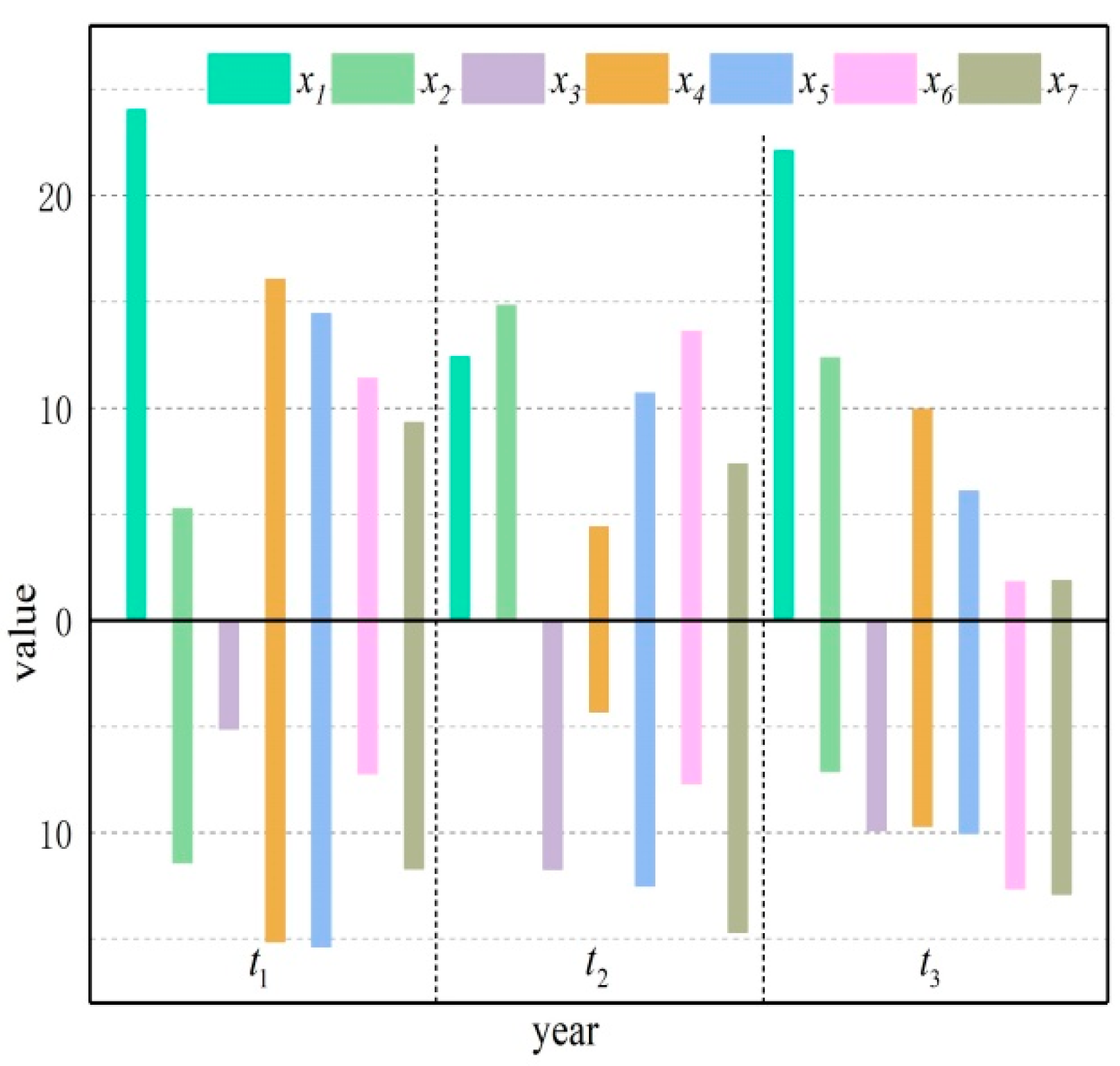
From Table 7, Table 8 and Table 9, it can be seen that the number of superiority-compatibility class elements is the largest in the POS domain, while the inferiority-compatibility class elements are the least in the NEG domain. According to Theorem 5, from t 1 to t 3 , the element with the most intersections in the superiority-compatibility class is x 3 , and the element with the most intersections in the inferiority-compatibility class is x 1 . The results are consistent with x 1 P O S and x 3 N E G . Moreover, the relationship between the superiority degree of the object and inferiority degree obtained according to R δ and R ε is shown in Figure 2, where the upper semi-axis of x represents the superiority degree and the lower semi-axis represents the inferiority degree. Taking t 1 as an example, element x 1 in the POS domain is completely in an advantageous position, and element x 3 in the NEG domain is completely in an inferior position. The superiority degree and inferiority degree of other elements are not balanced in t 1 - t 3 , which requires further analysis. From Table 10, Table 11 and Table 12 show the secondary decision evaluation of the BND domain.
To obtain the comprehensive evaluation results of the committee, the total number of decisions of different agroecological regions within t 1 - t 3 is compared, as shown in Figure 3.
In Figure 3, object x 1 has the highest acceptance rate, x 7 has a rejection rate of 70%, and the remaining delayed decision parts are also converted to reject decisions after the secondary decision. Similarly, object x 4 is transformed into an accept decision, and objects x 3 and x 5 are transformed into a reject decision after the second decision. Combined with Table 10, Table 11 and Table 12, the final decision result is shown in Table 13.
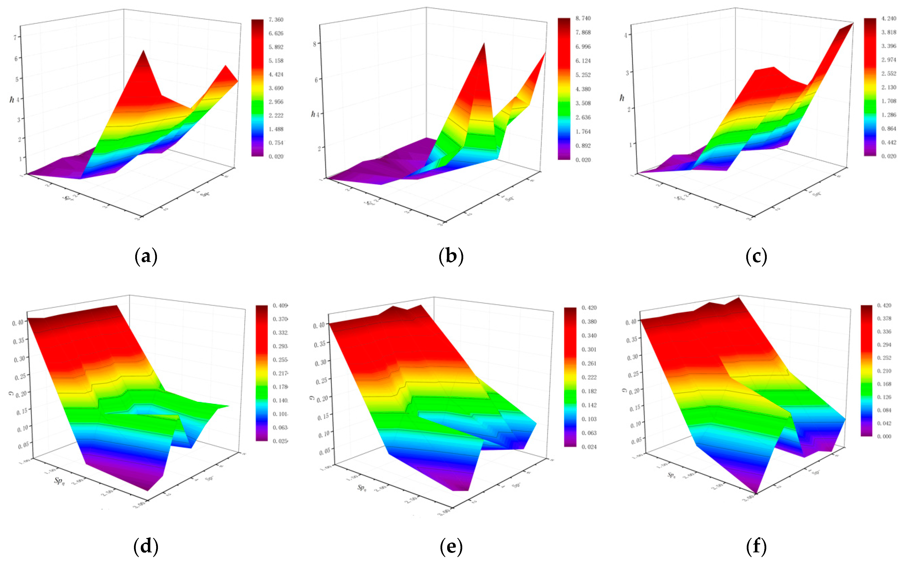
The final decision result of our model is that x 1 , x 2 , and x 4 regions can be invested, and x 3 , x 5 , x 6 , and x 7 regions cannot be directly invested. If we can only invest in one agroecological region in the POS domain, we can choose x 1 according to the relationship between superiority degree and inferiority degree, which is consistent with the results given in reference [57]. Although reference [58] did not further analyse the BND domain, based on the results of the POS domain and NEG domain, we believe that x 1 and x 4 are suitable for investment immediately and that x 7 is not suitable for investment. The only difference is in the decision division of the object x 2 . There are two possible reasons for our analysis: one is that reference [58] uses hypothetical conditional probability, which may cause our final results to be different, and the other is the effect of the state probability, as shown in Figure 4.
State possibility and advantage cost
Figure 4 shows the effect of state probability on advantage cost and information granularity by taking Q 1 as an example. We can find that the state possibility affects the formation of information granularity and indirectly affects the calculation of advantage cost. In addition, Figure 2 also shows that the change from t 1 to t 3 of object x 2 is unstable. All of these factors may cause inconsistency in the final decision of x 2 .

5. Conclusions

In this paper, we propose an IFTWD model based on the granular computing method. First, we construct the object information granularity by the relationship between the state probability distribution and the probability distribution. Second, to solve the problem of action and evaluation, a superiority-compatibility relation and inferiority-compatibility relation are proposed, and the decisions are divided. Finally, the calculation methods of superiority degree and inferiority degree are given and used for the secondary decision. This study extends the TAO model by using information granulation, decision stratification, and evaluation subdivision to analyse the uncertainty problem and construct a corresponding IFTWD model, which provides new ideas for the study of three-way granular computing and the three-way decision model under uncertain conditions. The next step will focus on the flexible properties and operator construction of three-way granular computing on intuitionistic fuzzy multiscale problems and the corresponding three-way decision model.

Author Contributions

X.X. initiated the research and wrote the paper, J.S. supervised the research work and provided helpful suggestions, and W.P. participated in some of these search work. All authors have read and agreed to the published version of the manuscript.

Funding

This research received no external funding.

Acknowledgments

This work is supported by the National Natural Science Foundation of China under Grant No. 61877004 and BNU Interdisciplinary Research Foundation for the First-Year Doctoral Candidates No. BNUXKJC1925.

Conflicts of Interest

The authors declare no conflict of interest.

References

  1. Pawlak, Z. Rough sets. Int. J. Comput. Inf. Sci. 1982, 11, 341–356. [Google Scholar] [CrossRef]
  2. Liu, K.Y.; Yang, X.B.; Yu, H.L.; Mi, J.S.; Wang, P.X.; Chen, X.J. Rough set based semi-supervised feature selection via ensemble selector. Knowl. Based Syst. 2019, 165, 282–296. [Google Scholar] [CrossRef]
  3. Jia, X.Y.; Li, W.W.; Shang, L. A multiphase cost-sensitive learning method based on the multiclass three-way decision-theoretic rough set model. Inf. Sci. 2019, 485, 248–262. [Google Scholar] [CrossRef]
  4. Greco, G.; Jipsen, P.; Manoorkar, K.; Palmigiano, A.; Tzimoulis, A. Logics for Rough Concept Analysis; ICLA 2019, Lecture Notes in Computer Science; Springer: Berlin/Heidelberg, Germany, 2019; pp. 144–159. [Google Scholar]
  5. Shao, M.W.; Guo, L.; Wang, C.Z. Connections between two-universe rough sets and formal concepts. Int. J. Mach. Learn. Cybern. 2018, 9, 1869–1877. [Google Scholar] [CrossRef]
  6. Wang, F.G.; Wang, N.B.; Cai, S.B.; Zhang, W.L. A similarity measure in formal concept analysis containing general semantic information and domain information. IEEE Access. 2020, 8, 75303–75312. [Google Scholar] [CrossRef]
  7. Yang, J.; Wang, G.Y.; Zhang, Q.H. Knowledge Distance Measure for the Multi-granularity Rough Approximations of a Fuzzy Concept. IEEE Trans. Fuzzy Syst. 2020, 28, 706–717. [Google Scholar] [CrossRef]
  8. Santra, D.; Basu, S.K.; Mandal, J.K.; Goswami, S. Rough set based lattice structure for knowledge representation in medical expert systems: Low back pain management case study. Expert Syst. Appl. 2020, 145, 113084. [Google Scholar] [CrossRef] [Green Version]
  9. Luqman, A.; Akram, M.; Koam, A.N.A. An m-Polar fuzzy hypergraph model of granular computing. Symmetry 2019, 11, 483. [Google Scholar] [CrossRef] [Green Version]
  10. Singh, P.; Huang, Y.P. A four-way decision-making approach using interval-valued fuzzy sets, rough set and granular computing: A new approach in data classification and decision-making. Granul. Comput. 2019, 1–13. [Google Scholar] [CrossRef]
  11. Pawlak, Z. Rough Sets: Theoretical Aspects of Resoning about Data; Kluwer Academic: Boston, MA, USA, 1991. [Google Scholar]
  12. Zhan, J.M.; Sun, B.Z.; Alcantud, J.C.R. Covering based multigranulation (I,T)-fuzzy rough set models and applications in multi-attribute group decision-making. Inf. Sci. 2019, 476, 290–318. [Google Scholar] [CrossRef]
  13. Yao, Y.Y.; Wong, S.K.M.; Lingras, P. A Decisions-Theoretic Rough Set Model. In 5th International Symposium of Methodologies for Intelligent Systems Held 25–27 October; North-Holland: New York, NY, USA, 1990; pp. 17–25. [Google Scholar]
  14. Li, M.M.; Chen, M.H.; Xu, W.H. Double-quantitative multigranulation decision-theoretic rough fuzzy set model. Int. J. Mach. Learn. Cybern. 2019, 10, 3225–3244. [Google Scholar] [CrossRef]
  15. Yu, J.H.; Li, Y.Q.; Chen, M.H.; Zhang, B.; Xu, W.H. Decision-theoretic rough set in lattice-valued decision information system. J. Intell. Fuzzy Syst. 2019, 36, 3289–3301. [Google Scholar] [CrossRef]
  16. Diker, M. Textures and fuzzy unit operations in rough set theory: An approach to fuzzy rough set models. Fuzzy Sets Syst. 2018, 336, 27–53. [Google Scholar] [CrossRef]
  17. Yao, Y.Y. Three-Way Decision: An Interpretation of Rules in Rough Set Theory. In Proceedings of the 4th International Conference on Rough Sets and Knowledge Technology, Gold Coast, Australia, 14–16 July 2009; pp. 642–649. [Google Scholar]
  18. Yao, Y.Y. Three-way decisions with probabilistic rough sets. Inf. Sci. 2010, 180, 341–353. [Google Scholar] [CrossRef] [Green Version]
  19. Yao, Y.Y. An Outline of a Theory of Three-Way Decisions. In Proceedings of the International Conference on Rough Sets and Current Trends in Computing, Chengdu, China, 17–20 August 2012; Volume 7413, pp. 1–17. [Google Scholar]
  20. Zhai, J.H.; Zhang, S.F. Three-way decisions model based on rough fuzzy set. J. Intell. Fuzzy Syst. 2018, 34, 2051–2059. [Google Scholar] [CrossRef]
  21. Zhao, X.R.; Hu, B.Q. Three-way decisions with decision-theoretic rough sets in multiset-valued information tables. Inf. Sci. 2020, 507, 684–699. [Google Scholar] [CrossRef]
  22. Yang, X.P.; Tan, A.H. Three-Way Decisions Based on Intuitionistic Fuzzy Sets. In Proceedings of the International Joint Conference on Rough Sets, Olsztyn, Poland, 3–7 July 2017; Springer: Cham, Switzerland, 2017; pp. 290–299. [Google Scholar]
  23. Liang, D.C.; Xu, Z.S.; Liu, D. Three-way decisions based on decision-theoretic rough sets with dual hesitant fuzzy information. Inf. Sci. 2017, 396, 127–143. [Google Scholar] [CrossRef]
  24. Liang, D.C.; Xu, Z.S.; Liu, D. Three-way decisions with intuitionistic fuzzy decision-theoretic rough sets based on point operators. Inf. Sci. 2017, 375, 183–201. [Google Scholar] [CrossRef]
  25. Gao, Y.; Li, D.S.; Zhong, H. A novel target threat assessment method based on three-way decisions under intuitionistic fuzzy multi-attribute decision making environment. Eng. Appl. Artif. Intell. 2020, 87, 103276. [Google Scholar] [CrossRef]
  26. Yang, X.P.; Li, T.J.; Tan, A.H. Three-way decisions in fuzzy incomplete information systems. Int. J. Mach. Learn. Cybern. 2020, 11, 664–674. [Google Scholar] [CrossRef]
  27. Liu, D.; Liang, D.C.; Wang, C.C. A novel three-way decision model based on incomplete information system. Knowl. Based Syst. 2016, 91, 32–45. [Google Scholar] [CrossRef]
  28. Zhang, H.Y.; Yang, S.Y.; Ma, J.M. Ranking interval sets based on inclusion measures and applications to three-way decisions. Knowl. Based Syst. 2016, 91, 62–70. [Google Scholar] [CrossRef]
  29. Wang, T.X.; Li, H.X.; Zhang, L.B.; Zhou, X.Z.; Huang, B. A Three-Way Decision Model Based on Cumulative Prospect Theory. Inf. Sci. 2020, 519, 74–92. [Google Scholar] [CrossRef]
  30. Yang, X.; Li, T.R.; Fujita, H.; Liu, D. A sequential three-way approach to multi-class decision. Int. J. Approx. Reason. 2019, 104, 108–125. [Google Scholar] [CrossRef]
  31. Qi, J.J.; Wei, L.; Yao, Y.Y. Three-Way Formal Concept Analysis. In Proceedings of the International Conference on Rough Sets and Knowledge Technology, Shanghai, China, 24–26 October 2014; Spring: Berlin/Heidelberg, Germany, 2014; pp. 732–741. [Google Scholar]
  32. Yu, H.Y.; Li, Q.G.; Cai, M.J. Characteristics of three-way concept lattices and three-way rough concept lattices. Knowl. Based Syst. 2018, 146, 181–189. [Google Scholar] [CrossRef]
  33. Yu, H.; Wang, X.C.; Wang, G.Y.; Zeng, X.H. An active three-way clustering method via low-rank matrices for multi-view data. Inf. Sci. 2020, 507, 823–839. [Google Scholar] [CrossRef]
  34. Wang, P.X.; Yao, Y.Y. CE3: A three-way clustering method based on mathematical morphology. Knowl. Based Syst. 2018, 155, 54–65. [Google Scholar] [CrossRef]
  35. Xu, J.F.; Zhang, Y.J.; Miao, D.Q. Three-way confusion matrix for classification: A measure driven view. Inf. Sci. 2020, 507, 772–794. [Google Scholar] [CrossRef]
  36. Zhang, Y.B.; Miao, D.Q.; Wang, J.Q.; Zhang, Z.F. A cost-sensitive three-way combination technique for ensemble learning in sentiment classification. Int. J. Approx. Reason. 2019, 105, 85–97. [Google Scholar] [CrossRef]
  37. Ma, X.A.; Zhao, X.R. Cost-sensitive three-way class-specific attribute reduction. Int. J. Approx. Reason. 2019, 105, 153–174. [Google Scholar] [CrossRef]
  38. Zhang, X.Y.; Yang, J.L.; Tang, L.Y. Three-way class-specific attribute reducts from the information viewpoint. Inf. Sci. 2020, 507, 840–872. [Google Scholar] [CrossRef]
  39. Fang, Y.; Min, F. Cost-sensitive approximate attribute reduction with three-way decisions. Int. J. Approx. Reason. 2019, 104, 148–165. [Google Scholar] [CrossRef]
  40. Liang, D.C.; Wang, M.W.; Xu, Z.S.; Liu, D. Risk appetite dual hesitant fuzzy three-way decisions with TODIM. Inf. Sci. 2020, 507, 585–605. [Google Scholar] [CrossRef]
  41. Xue, Z.A.; Xin, X.W.; Yuan, Y.L.; Xue, T.Y. Intuitionistic fuzzy possibility measure-based three-way decisions for incomplete data. J. Intell. Fuzzy Syst. 2018, 35, 5657–5666. [Google Scholar] [CrossRef]
  42. Yao, Y.Y. Three-way conflict analysis: Reformulations and extensions of the Pawlak model. Knowl. Based Syst. 2019, 180, 26–37. [Google Scholar] [CrossRef]
  43. Sun, B.Z.; Chen, X.T.; Zhang, L.Y.; Ma, W.M. Three-way decision making approach to conflict analysis and resolution using probabilistic rough set over two universes. Inf. Sci. 2020, 507, 809–822. [Google Scholar] [CrossRef]
  44. Zadeh, L.A. Toward a theory of fuzzy information granulation and its centrality in human reasoning and fuzzy logic. Fuzzy Sets Syst. 1997, 90, 111–127. [Google Scholar] [CrossRef]
  45. Yao, Y.Y. A Unied Framework of Granular Computing. Handbook of Granular Computing; John Wiley & Sons: Hoboken, NJ, USA, 2008; pp. 401–410. [Google Scholar]
  46. Yao, Y.Y. A triarchic theory of granular computing. Granul. Comput. 2016, 1, 145–157. [Google Scholar] [CrossRef] [Green Version]
  47. Leng, J.W.; Chen, Q.X.; Mao, N.; Jiang, P.Y. Combining granular computing technique with deep learning for service planning under social manufacturing contexts. Knowl. Based Syst. 2018, 143, 295–306. [Google Scholar] [CrossRef]
  48. Loia, V.; Orciuoli, F.; Pedrycz, W. Towards a granular computing approach based on formal concept analysis for discovering periodicities in data. Knowl. Based Syst. 2018, 146, 1–11. [Google Scholar] [CrossRef]
  49. Lu, W.; Zhou, W.; Shan, D.; Zhang, L.Y.; Yang, J.H.; Liu, X.D. The linguistic modeling of interval-valued time series: A perspective of granular computing. Inf. Sci. 2019, 478, 476–498. [Google Scholar] [CrossRef]
  50. Fang, Y.; Gao, C.; Yao, Y.Y. Granularity-driven sequential three-way decisions: A cost-sensitive approach to classification. Inf. Sci. 2020, 507, 644–664. [Google Scholar] [CrossRef]
  51. Yao, Y.Y. Three-way decision and granular computing. Int. J. Approx. Reason. 2018, 103, 107–123. [Google Scholar] [CrossRef]
  52. Yao, Y.Y. Three-way granular computing, rough sets, and formal concept analysis. Int. J. Approx. Reason. 2020, 116, 106–125. [Google Scholar] [CrossRef]
  53. Yao, Y.Y. Tri-level thinking: Models of three-way decision. Int. J. Mach. Learn. Cybern. 2019, 1–13. [Google Scholar] [CrossRef]
  54. Atanassov, K.T. Intuitionistic fuzzy sets. Fuzzy Sets Syst. 1986, 20, 87–96. [Google Scholar] [CrossRef]
  55. Greco, S.; Matarazzo, B.; Slowinski, R. Rough approximation by dominance relations. Int. J. Intell. Syst. 2002, 17, 153–171. [Google Scholar] [CrossRef]
  56. Liu, J.B.; Zhou, X.Z.; Huang, B.; Li, H.X. A Three-Way Decision Model Based on Intuitionistic Fuzzy Decision Systems. In Proceedings of the International Joint Conference on Rough Sets, Olsztyn, Poland, 3–7 July 2017; Springer: Cham, Switzerland, 2017; pp. 249–263. [Google Scholar]
  57. Xu, Z.S.; Yager, R.R. Dynamic intuitionistic fuzzy multi-attribute decision making. Int. J. Approx. Reason. 2008, 48, 246–262. [Google Scholar] [CrossRef] [Green Version]
  58. Liang, D.C.; Liu, D. Deriving three-way decisions from intuitionistic fuzzy decision-theoretic rough sets. Inf. Sci. 2015, 300, 28–48. [Google Scholar] [CrossRef]
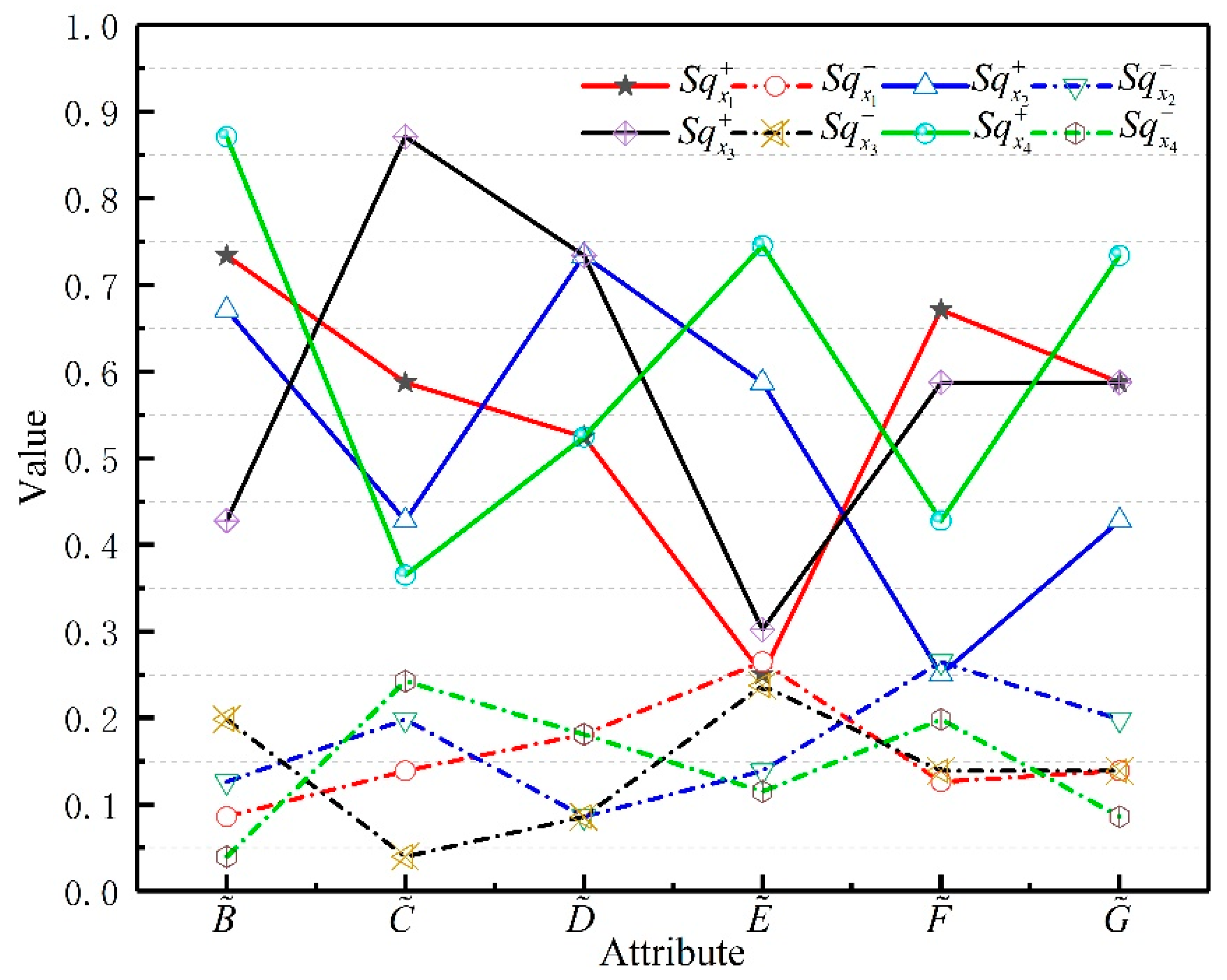
Figure 1. Membership state possibility and non-membership state possibility.
Symmetry 12 01068 g001
Figure 2. Advantages and disadvantages of each agroecological region between t1t3.
Symmetry 12 01068 g002
Figure 3. Acceptance rate, rejection rate and delay rate in the secondary decision.
Symmetry 12 01068 g003
Figure 4. 3D vector illustration of indicator Q 1 . (a) ( t 1 : S q + , S q , ħ ) , (b) ( t 2 : S q + , S q , ħ ) , (c) ( t 3 : S q + , S q , ħ ) . State possibilities and information granularity, (d) ( t 1 : S q η , S q , G ) , (e) ( t 2 : S q η , S q , G ) , (f) ( t 3 : S q η , S q , G ) .
Symmetry 12 01068 g004
Table 1. Cost function matrix.
ActionCost Function
X ¬ X
a P λ P P λ P N
a B λ B P λ B N
a N λ N P λ N N
Table 2. Intuitionistic fuzzy decision system based on security audit risk assessment.
B ˜ C ˜ D ˜ E ˜ F ˜ G ˜
x 1 (0.8, 0.2)(0.7, 0.3)(0.6, 0.3)(0.5, 0.5)(0.7, 0.2)(0.7, 0.3)
x 2 (0.7, 0.2)(0.6, 0.4)(0.8, 0.2)(0.7, 0.3)(0.5, 0.5)(0.6, 0.4)
x 3 (0.6, 0.4)(0.9, 0.1)(0.8, 0.2)(0.4, 0.6)(0.7, 0.3)(0.7, 0.3)
x 4 (0.9, 0.1)(0.4, 0.2)(0.6, 0.3)(0.7, 0.1)(0.6, 0.4)(0.8, 0.2)
Table 3. Relationship between state probability distribution and probability distribution.
Comparison and Classification of ValuesProbability Distributions
ν B ˜ ( x i ) > S q B ˜ ( x i ) P 1 ( μ B ˜ ( x i ) , ν B ˜ ( x i ) ) = { x i U | ( S q B ˜ + ( x i ) > μ B ˜ ( x i ) ) ( ν B ˜ ( x i ) > S q B ˜ ( x i ) ) }
S q B ˜ + ( x i ) > μ B ˜ ( x i ) ν B ˜ ( x i ) = S q B ˜ ( x i ) P 2 ( μ B ˜ ( x i ) , ν B ˜ ( x i ) ) = { x i U | ( S q B ˜ + ( x i ) > μ B ˜ ( x i ) ) ( ν B ˜ ( x i ) = S q B ˜ ( x i ) ) }
ν B ˜ ( x i ) < S q B ˜ ( x i ) P 3 ( μ B ˜ ( x i ) , ν B ˜ ( x i ) ) = { x i U | ( S q B ˜ + ( x i ) > μ B ˜ ( x i ) ) ( ν B ˜ ( x i ) < S q B ˜ ( x i ) ) }
ν B ˜ ( x i ) > S q B ˜ ( x i ) P 4 ( μ B ˜ ( x i ) , ν B ˜ ( x i ) ) = { x i U | ( S q B ˜ + ( x i ) = μ B ˜ ( x i ) ) ( ν B ˜ ( x i ) > S q B ˜ ( x i ) ) }
S q B ˜ + ( x i ) = μ B ˜ ( x i ) ν B ˜ ( x i ) = S q B ˜ ( x i ) P 5 ( μ B ˜ ( x i ) , ν B ˜ ( x i ) ) = { x i U | ( S q B ˜ + ( x i ) = μ B ˜ ( x i ) ) ( ν B ˜ ( x i ) = S q B ˜ ( x i ) ) }
ν B ˜ ( x i ) < S q B ˜ ( x i ) P 6 ( μ B ˜ ( x i ) , ν B ˜ ( x i ) ) = { x i U | ( S q B ˜ + ( x i ) = μ B ˜ ( x i ) ) ( ν B ˜ ( x i ) < S q B ˜ ( x i ) ) }
ν B ˜ ( x i ) > S q B ˜ ( x i ) P 8 ( μ B ˜ ( x i ) , ν B ˜ ( x i ) ) = { x i U | ( S q B ˜ + ( x i ) < μ B ˜ ( x i ) ) ( ν B ˜ ( x i ) = S q B ˜ ( x i ) ) }
S q B ˜ + ( x i ) < μ B ˜ ( x i ) ν B ˜ ( x i ) = S q B ˜ ( x i ) P 7 ( μ B ˜ ( x i ) , ν B ˜ ( x i ) ) = { x i U | ( S q B ˜ + ( x i ) < μ B ˜ ( x i ) ) ( ν B ˜ ( x i ) > S q B ˜ ( x i ) ) }
ν B ˜ ( x i ) < S q B ˜ ( x i ) P 9 ( μ B ˜ ( x i ) , ν B ˜ ( x i ) ) = { x i U | ( S q B ˜ + ( x i ) < μ B ˜ ( x i ) ) ( ν B ˜ ( x i ) < S q B ˜ ( x i ) ) }
Table 4. Approximate division of information granularity based on state probability.
C 1 : P b i g ( x i ) S q b i g ( x i ) C 2 : S q s m a l l ( x i ) P s m a l l ( x i )
Fine-grained: G F OO
Medium-grained: G M O( × ) × (O)
Coarse-grained: G C × ×
Table 5. Information granularity of each domain object in Table 2.
μ ν P ( x i ) D ( S q max + , P ) D ( S q min , P ) G ( x i )
x 1 0.860.270.240.520.16 G F
x 2 0.860.270.270.480.13 G M
x 3 0.920.140.270.620.13 G M
x 4 0.920.140.220.670.18 G M
Table 6. Information related to each object classification.
[ x i ] R δ [ x i ] R ε R _ ( x i ) R ¯ ( X ) Classification
x 1 { x 2 , x 3 , x 4 } { ϕ } { x 1 } { ϕ } P O S
x 2 { x 4 } { x 1 , x 3 } { ϕ } { ϕ } B N D
x 3 { x 2 , x 4 } { x 1 } { ϕ } { ϕ } B N D
x 4 { ϕ } { x 1 , x 3 } { ϕ } { x 4 } N E G
Table 7. Division results of the agroecological region in t 1 .
[ x i ] R δ [ x i ] R ε P ( x i ) P G ( x i ) Classification
x 1 { x 2 , x 3 , x 4 , x 5 , x 6 , x 7 } { ϕ } 0.07 G F POS
x 2 { x 3 } { x 1 , x 4 , x 5 , x 6 , x 7 } 0.15 G M BND
x 3 { ϕ } { x 1 , x 4 , x 5 } 0.2 G M NEG
x 4 { x 2 , x 3 , x 5 , x 7 } { x 1 , x 5 } 0.08 G F BND
x 5 { x 2 , x 3 , x 7 } { x 1 , x 4 } 0.1 G F BND
x 6 { x 2 , x 3 , x 7 } { x 1 } 0.15 G C BND
x 7 { x 2 , x 3 } { x 1 , x 4 , x 5 , x 6 } 0.25 G M BND
Table 8. Division results of the agroecological region in t 2 .
[ x i ] R δ [ x i ] R ε P ( x i ) G ( x i ) Classification
x 1 { x 3 , x 5 , x 6 , x 7 } { ϕ } 0.08 G F POS
x 2 { x 3 , x 5 , x 6 , x 7 } { ϕ } 0.09 G F POS
x 3 { ϕ } { x 1 , x 2 , x 4 , x 5 , x 6 , x 7 } 0.14 G M NEG
x 4 { x 3 , x 7 } { x 1 } 0.11 G F BND
x 5 { x 3 , x 7 } { x 1 , x 2 , x 6 } 0.16 G M BND
x 6 { x 3 , x 5 , x 7 } { x 1 , x 2 } 0.22 G M BND
x 7 { x 3 } { x 1 , x 2 , x 4 , x 5 , x 6 } 0.20 G M BND
Table 9. Division results of the agroecological region in t 3 .
[ x i ] R δ [ x i ] R ε P ( x i ) G ( x i ) Classification
x 1 { x 2 , x 3 , x 4 , x 5 , x 6 , x 7 } { ϕ } 0.06 G F POS
x 2 { x 3 , x 5 , x 6 , x 7 } { x 1 } 0.08 G F BND
x 3 { ϕ } { x 1 , x 2 , x 4 , x 5 , x 6 , x 7 } 0.17 G M NEG
x 4 { x 3 , x 5 , x 6 , x 7 } { x 1 , x 2 } 0.09 G F BND
x 5 { x 3 , x 5 , x 6 , x 7 } { x 1 , x 2 , x 4 } 0.14 G M BND
x 6 { x 7 } { x 1 , x 2 , x 4 , x 5 , x 7 } 0.24 G M BND
x 7 { x 6 } { x 1 , x 2 , x 4 , x 5 , x 6 } 0.22 G M BND
Table 10. Agroecological region secondary decision in t 1 .
InitializationFirst CycleSecond CycleFinal Result
POS { x 1 } { x 1 , x 6 } { x 1 , x 4 , x 6 } { x 1 , x 4 , x 6 }
BND { x 2 , x 4 , x 5 , x 6 , x 7 } { x 4 , x 5 , x 7 } { x 5 } { ϕ }
NEG { x 3 } { x 2 , x 3 } { x 2 , x 3 , x 7 } { x 2 , x 3 , x 5 , x 7 }
Table 11. Agroecological region secondary decision in t 2
InitializationFirst CycleSecond CycleFinal Result
POS { x 2 } { x 1 , x 2 } { x 1 , x 2 , x 6 } { x 1 , x 2 , x 4 , x 6 }
BND { x 1 , x 4 , x 5 , x 6 , x 7 } { x 4 , x 5 , x 6 } { x 4 } { ϕ }
NEG { x 3 } { x 3 , x 7 } { x 3 , x 5 , x 7 } { x 3 , x 5 , x 7 }
Table 12. Agroecological region secondary decision in t 3 .
InitializationFirst CycleSecond CycleFinal Result
POS { x 1 } { x 1 , x 2 } { x 1 , x 2 , x 4 } { x 1 , x 2 , x 4 }
BND { x 2 , x 3 , x 4 , x 5 , x 6 } { x 3 , x 4 , x 5 } { x 5 } { ϕ }
NEG { x 7 } { x 6 , x 7 } { x 3 , x 6 , x 7 } { x 3 , x 5 , x 6 , x 7 }
Table 13. Final decision result.
Region x 1 x 2 x 3 x 4 x 5 x 6 x 7
DecisionPOSPOSNEGPOSNEGNEGNEG