Abstract
A vital role in the dynamics of physical systems is played by symmetries. In fact, these studies require the solution for systems of equations on abstract spaces including on the finite-dimensional Euclidean, Hilbert, or Banach spaces. Methods of iterative nature are commonly used to determinate the solution. In this article, such methods of higher convergence order are studied. In particular, we develop a two-step iterative method to solve large scale systems that does not require finding an inverse operator. Instead of the operator’s inverting, it uses a two-step Schultz approximation. The convergence is investigated using Lipschitz condition on the first-order derivatives. The cubic order of convergence is established and the results of the numerical experiment are given to determine the real benefits of the proposed method.
Keywords:
nonlinear equation; iterative method; approximation of inverse operator; local convergence; order of convergence; Lipschitz condition MSC:
65H10; 65J15; 47H17
1. Introduction
In this article, F denotes an operator acting on a Banach space X with values inside a Banach space Y and is convex. To find the approximate solution p of
we often utilize the method [1,2,3,4,5]
due to Newton or its differential or difference modifications. Iterative methods are used since p can be found in closed form only in special cases. That is the first benefit of using iterative methods. However, at each iteration, it is necessary to find one or more inverse operators. This is one setback for using Newton-type methods [1,2,3,4,5]. Since it is not always easy to do, we bypass this obstacle by finding approximations for inversion using only multiplications of linear operators. This is one major benefit. There is the novelty of our paper, since we contribute in this direction.
Methods with approximation of inverse operator are based on different ideas. Some ideas intend to construct approximations to the solution of a nonlinear Equation (1), and others to construct approximations to the inverse operator. There are two approaches to approximate an inverse operator: successive approximation (SA) and parallel (synchronous and asynchronous) approximations. In methods with the successive approximation, the calculations in separate branches are performed alternately. In methods with the parallel approximation requiring the computation of an inverse of a linear operator, the computations in separate branches of the method are performed in parallel. Such methods are effective for numerically solving Equation (1) in the parallel processor system with common memory [6,7,8].
Many authors have investigated methods with SA of inverse operator. For example, the local convergence of modifications of Newton and Steffensen methods are studied in [9]. In [10,11,12], the authors studied the semilocal convergence (SLC) for Ulm method [9]
and its difference analog
Here, E is the identity operator in X and stands for the first-order divided difference for operator [13]. Moreover, and are initial approximations for a solution and an inverse operator , respectively. Furthermore, the closer and are to p, the better Equation (4) performs. However, there are no preconditioners. An investigation of the accelerated Newton method and a two-parametric secant-type method with SA of the inverse operator is performed in [14,15] (see also [16,17,18]). It is worth noting that Ulm type methods provide the same order of convergence as Newton’s or Steffensen’s but without using inverses which are very expensive to compute in general. In certain cases, even the ratio of convergence may be smaller (see the numerical section).
A method with synchronous inverse approximation
and a method with the asynchronous approximation were considered by A. Rooze [6,7]. Some modifications of a method by Gauss–Newton with SA of the inverse operator to solve a nonlinear least squares problems were proposed by Iakymchuk, Shakhno [8].
In 1983, the authors built third-, fifth-, and sixth-order methods with approximation of inverse operator for solving operator Equations [19]. In particular, the third-order method has the form
where is a real parameter.
To increase the order of convergence, efficiency and applicability of the aforementioned Ulm-type method, by replacing the divided differences by Fréchet derivatives in Equation (6), we develop the method
This method is a two-step modification of Newton method [2,20]:
It is easy to see that the method in Equation (7) coincides with the third-order iterative process
which was proposed by Esquerro, Hernández [21]. They only investigated the semilocal convergence (SLC) of the method in Equation (9). Obviously, the methods in Equations (7) and (9) can be considered as methods SA for inverse operator.
We examine conditions for local convergence (LC) of the method in Equation (7) including its convergence order. We note that LC results are very important, since they demonstrate the degree of difficulty in selecting starters that guarantee convergence to p.
Another novelty of the developed method in Equation (7) lies in the fact that the inverse at each step is not calculated compared to other methods; the method is suitable to solve large scale systems; and it has better rate and convergence order than other methods using related information (see also benefits reported in Section 3. Indeed, there are significant developments in the study of Ulm-type methods. Moreover, these ideas can be used to expand the applicability of other methods along the same lines.
Section 2 contains the LC study of method in Equation (7). Large scale systems are solved in Section 3, where X and Y are specialized to be finite-dimensional Euclidean spaces. The study of solving large scale systems is of extreme importance, since most problems from diverse disciplines reduce to solving such systems [1,2,3,4,5,6,7,8,9,10,11,12,13,14,15,16,17,18,19,20,21,22].
2. LC study for the Method in Equation (7)
The following theorem establishes the conditions under which the iterative process in Equation (7) is convergent.
Theorem 1.
Assume that:
Proof.
The proof is performed by mathematical induction.
It follows from
that , and the estimate in Equation (14) is true for . Suppose that and the estimate in Equation (14) is satisfied for . It follows that , since is provided by Equation (13). Taking into account Equation (10) and the definition , we get
We obtain from the first equality of Equation (7) and the Taylor’s formula
In addition, , and whence it follows .
We obtain from the second equality of Equation (7) and the Taylor’s formula
Hence, we have, given the conditions in Equations (10)–(12) and the estimates in Equations (15), (17), and (18),
Thus, , since .
On the other hand, based on the third formula of Equation (7)
In accordance with the fourth equality of Equation (7),
From this relationships, based on the conditions in Equations (11) and (12) and estimates in Equations (20) and (21), we get in turn
That is, Equation (14) is fulfilled for an iteration . The induction is complete.
Moreover, it follows from the estimate in Equation (14) for the convergence of sequences and . ☐
Next, a uniqueness result follows.
Proposition 1.
Suppose: Equation (1) has a solution , where is convex and
Set and .
Then, p uniquely solves (1) on S.
Proof.
Consider for with , operator . Using Equation (23), we obtain
thus T is invertible. Hence, follows from
☐
The method in Equation (7) has a higher convergence rate than the Newton and Steffensen method. Moreover, in contrast, it does not require an inverse operator. Furthermore, the convergence order of method in Equation (7) is larger than for methods with the successive approximation in Equations (3) and (4).
3. Numerical Experiments
We used large scale test problems from Luksan [22] for the numerical study of the methods. Calculations were performed in Octave 5.1.0. Stopping iterative processes occurred under the condition
The initial approximations were calculated by the rules , . We compared methods by the number of iterations required to obtain an approximate solution. Table 1 shows the results for .

Table 1.
The number of iterations for different values of s.
Example 1.
Trigonometric-exponential function.
Example 2.
Consider tridiagonal function due to Broyden.
Example 3.
Counter current reactor problem.
The comparison by the number of iterations was performed to confirm the theoretical results about the higher convergence order of the studied method in Equation (7) than for the Ulm method in Equation (3). Obtained results also show that the methods with the approximation of inverse operator are somewhat inferior to the corresponding methods with the calculation of the inverse operator. However, the benefit of these methods is that they can be used when finding the inverse operator is impossible or difficult.
The graphs show the values of error at each iteration (see Figure 1). These are results for for Example 1, for Example 2, and for Example 3. We draw graphs using a logarithmic scale for both of the axes.
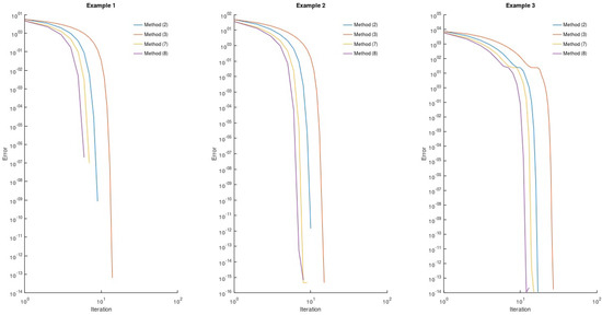
Figure 1.
The error at each iteration.
We see from the results on graphs that the errors of the methods with the approximation of inverse operator in Equations (3) and (7) decrease more slowly than for the basic methods in Equations (2) and (8), respectively. Moreover, obtained numerical results confirm that the methods in Equations (7) and (8) have a higher convergence rate than those in Equations (2) and (3).
4. Conclusions
The LC of method in Equation (7) with approximation of inverse operator for solving large scaled systems of equations is studied. The cubic order and radius of convergence of this method are determined. Numerical results are presented which demonstrate the computational benefits of the method.
Author Contributions
Conceptualization, S.S.; Investigation, I.K.A., S.S., and H.Y.; and Editing, I.K.A. All authors have read and agreed to the published version of the manuscript.
Funding
This research received no external funding.
Conflicts of Interest
The authors declare no conflict of interest.
References
- Argyros, I.K. Convergence and Applications of Newton-Type Iterations; Springer: New York, NY, USA, 2008; 506p. [Google Scholar]
- Amat, S.; Busquier, S.; Plaza, S. Review of some iterative root–finding methods from a dynamical point of view. Ser. A Math. Sci. 2004, 10, 3–35. [Google Scholar]
- Amat, S.; Busquier, S.; Plaza, S. Dynamics of King’s and Jarratt iterations. Aequ. Math. 2005, 69, 212–223. [Google Scholar] [CrossRef]
- Kantorovich, L.V.; Akilov, G.P. Functional Analysis; Nauka: Moscow, Russia, 1977; 744p. [Google Scholar]
- Magrenan, A.A. Different anomalies in a Jarratt family of root-finding methods. Appl. Math. Comput. 2014, 233, 29–38. [Google Scholar]
- Rooze, A.F. An iterative method for solving nonlinear equations using parallel inverse operator approximation. Izv. Acad. Nauk Est. SSR Fiz. Mat. 1982, 31, 32–37. (In Russian) [Google Scholar]
- Rooze, A.F. An asynchronous iteration method of solving non-linear equations using parallel approximation of an inverse operator. USSR Comput. Math. Math. Phys. 1986, 26, 188–191. (In Russian) [Google Scholar] [CrossRef]
- Iakymchuk, R.; Shakhno, S. Methods with successive and parallel approximations of inverse operator for the nonlinear least squares problem. Proc. Appl. Math. Mech. 2015, 15, 569–570. [Google Scholar] [CrossRef][Green Version]
- Ulm, S. On iterative methods with successive approximation of the inverse operator. Izv. Acad. Nauk Est. SSR Fiz. Mat. 1967, 16, 403–411. (In Russian) [Google Scholar]
- Argyros, I.K. On Ulm’s method for Fréchet differentiable operators. J. Appl. Math. Comput. 2005, 31, 97–111. [Google Scholar] [CrossRef]
- Argyros, I.K. On Ulm’s method using divided differences of order one. Numer. Algorithms 2009, 52, 295–320. [Google Scholar] [CrossRef]
- Burmeister, W. Inversionfreie Verfahren zur Lösung nichtlinearer Operatorgleichungen. ZAMM 1972, 52, 101–110. [Google Scholar] [CrossRef]
- Ulm, S. On generalized divided differences. Izv. Acad. Nauk. Est. SSR Fiz. Mat. 1967, 16, 13–26. (In Russian) [Google Scholar]
- Shakhno, S.M. Convergence of one iterative method with successive approximation of inverse operator. Visnyk Lviv. Univ. Ser. Mech. Math. 1989, 31, 62–66. (In Ukrainian) [Google Scholar]
- Shakhno, S.M.; Yarmola, H.P. Two-step secant type method with approximation of the inverse operator. Carpathian Math. Publ. 2013, 5, 150–155. (In Ukrainian) [Google Scholar] [CrossRef][Green Version]
- Vaarmann, O. On some iterative methods with successive approximation of the inverse operator. I. Izv. Acad. Nauk Est. SSR Fiz. Mat. 1968, 17, 379–387. (In Russian) [Google Scholar]
- Verzhbitskiy, V.M. Iterative methods with successive approximation of inverse operators. Izv. IMI UdGU 2006, 2, 129–138. (In Russian) [Google Scholar]
- Vaarmann, O. On some iterative methods with successive approximation of the inverse operator. II. Izv. Acad. Nauk Est. SSR Fiz. Mat. 1969, 18, 14–21. (In Russian) [Google Scholar]
- Vasilyev, F.P.; Khromova, L.M. On high-order methods for solving operator equations. Dokl. Nauk SSSR 1983, 270, 28–31. (In Russian) [Google Scholar]
- Esquerro, J.A.; Hernández, M.A.; Salanova, M.A. A discretization scheme for some conservative problems. J. Comp. Appl. Math. 2000, 115, 181–192. [Google Scholar] [CrossRef]
- Esquerro, J.A.; Hernández, M.A. An Ulm-type method with R-order of convergence three. Nonlinear Anal. Real World Appl. 2012, 12, 14–26. [Google Scholar] [CrossRef]
- Luksan, L. Inexact trust region method for large sparse systems of nonlinear equations. J. Optim. Theory Appl. 1994, 81, 569–590. [Google Scholar] [CrossRef][Green Version]
© 2020 by the authors. Licensee MDPI, Basel, Switzerland. This article is an open access article distributed under the terms and conditions of the Creative Commons Attribution (CC BY) license (http://creativecommons.org/licenses/by/4.0/).