On the Integration of Stiff ODEs Using Block Backward Differentiation Formulas of Order Six

Abstract

In this research, a six-order, fully implicit Block Backward Differentiation Formula with two off-step points (BBDFO(6)), for the integration of first-order ordinary differential equations (ODEs) that exhibit stiffness, is proposed. The order, consistency and stability properties of the method are discussed, and the method is found to be zero stable and consistent. Hence, the method is convergent. The numerical comparisons with the existing methods of a similar type are given to demonstrate the accuracy of the derived method.

1. Introduction

In this paper, we consider the numerical solution of the first order initial value problem (IVP) of ordinary differential equations (ODEs) in the form of

$$y^{\prime }\left(x\right)=f\left(x,y\right), y\left(a\right)=\mu , x\in \left[a,b\right]$$

(1)

where $y^T=\left(y_1\left(x\right),y_2\left(x\right),\dots ,y_d\left(x\right)\right),f^T=\left(f_1\left(x\right),f_2\left(x\right),\dots ,f_d\left(x\right)\right)$ and ${\mu }^T=\left({\mu }_1\left(x\right),{\mu }_2\left(x\right),\dots ,{\mu }_d\left(x\right)\right).$ Equation (1) is said to be linear if $f\left(x,y\right)=A\left(x\right)y+\mathsf{\Phi }\left(x\right),$ where $A\left(x\right)$ is a constant $d\times d$ matrix and $\mathsf{\Phi }\left(x\right)$ is a d-dimensional vector assumed to be continuously differentiable, and if it satisfies the Lipschitz conditions as given in [1], which guarantees the existence and uniqueness of the solution of Equation (1).

The development of numerical methods for the solution of Equation (1) is influenced by the types of ODEs, such as linear or non-linear ODEs, or stiff or non-stiff ODEs. Note that using the wrong type of method for a model can produce slow and/or inaccurate results. Generally, the problems in the form of Equation (1) can be classified into two types. The first type is non-stiff ODEs, for which all of the components evolve simultaneously and on comparable time-scales. Non-stiff problems are often solved by using explicit methods with some error control. The second type is stiff ODEs. The first appearance of the term “stiff” is in the paper by [2] on the problems in chemical kinetics. There are various definitions of stiffness given in the literature since there is no universally accepted definition. The problem in Equation (1) is said to be describing the stiff problem if:

• It contains widely varying time scales, i.e., some components of the solution decay much more rapidly than others [3];
• The step size is dictated by the stability requirements rather than the accuracy requirements [3];
• Explicit methods do not work, or work only extremely slowly [4];
• All of its eigenvalues have negative real parts, and the stiffness ratio (the ratio of the magnitudes of the real parts of the largest and smallest eigenvalues) is large [3];
• No solution component is unstable (no eigenvalue of the Jacobian matrix has a real part which is at all large and positive) and at least some components are very stable (at least one eigenvalue has a real part which is large and negative) [5].

For this article, we consider the definition of stiffness to be that given by [6] which stated that the linear system of Equation (1) is said to be stiff if,

(i)

$Re\left({\lambda }_i\right)<0,i=1,2,\dots ,d$ and

(ii)

$\underset{i}{\max }\left|Re\left({\lambda }_i\right)\right|\gg \underset{i}{\min }\left|Re\left({\lambda }_i\right)\right|,$ where ${\lambda }_i$ are the eigenvalues of A and the ratio $S=\underset{i}{\max }\left|Re\left({\lambda }_i\right)\right|/\underset{i}{\min }\left|Re\left({\lambda }_i\right)\right|$ is called the stiffness ratio as a measure of stiffness.

The consideration of stability properties is particularly important when developing methods for solving stiff ODEs, and implicit methods which possess an A-stable region are preferred. Several numerical methods of various types have been proposed for the integration of both types of problems in Equation (1). Among the most popular and widely used methods for the solution of the stiff systems in Equation (1) are the Backward Differentiation Formulas (BDFs) proposed by [7]. In MATLAB, Gear’s methods are implemented in the stiff solver ode15s.

For many years, the development of more advanced and efficient methods for the solution of ordinary differential equations (ODEs) has been an active research area. Most of the developments have been based on block methods. These block methods generate multiple solutions simultaneously and in single iterations. As noted by [8,9,10,11,12,13,14,15,16,17,18], these methods are effective for solving the problems in Equation (1). The block methods not only reduce the computational time but also require a smaller number of function evaluations per step. These block methods include the variable order Adams methods, the Runge–Kutta methods and Backward Differentiation Formulas. Inspired by Gear’s method, [11,12,13,14,15,16,17,18] developed Block Backward Differentiation Formulas (BBDFs) which are proven to be efficient in solving stiff ODEs. For a detailed study on the theory and development of BBDFs, one can refer to [19]. Recently, the method that incorporated a BBDF proposed by [11] has been modified and extended, and it is now an improved method due to its enhancements in reducing the total number of integration steps and computational time, and in providing better accuracy of the approximation—see [12,20]. Therefore, in this paper, we formulate a new method called the Block Backward Differentiation Formula with two off-step points (BBDFO(6)) which is extended from the BBDF method developed by [14] by adding off-step points. These block methods with off-steps were studied by [21]. A closely related method with off-step points was described by [22,23,24]. A similar approach is adapted from [25,26] in adjusting the selection of the most suitable off-step points. We extend the theory to [11] and establish new coefficients of stability which is an improvement on the work of [21]. We shall restrict our discussion to solving stiff ODEs.

This paper is organized as follows: in Section 2, we present the derivation of the coefficients of the new method; Section 3 includes the order, zero stability, and region of stability of the proposed method. In Section 4, numerical tests are performed on the first-order differential equation problems possessing stiffness and are compared to related works. Finally, the conclusions are presented in Section 5.

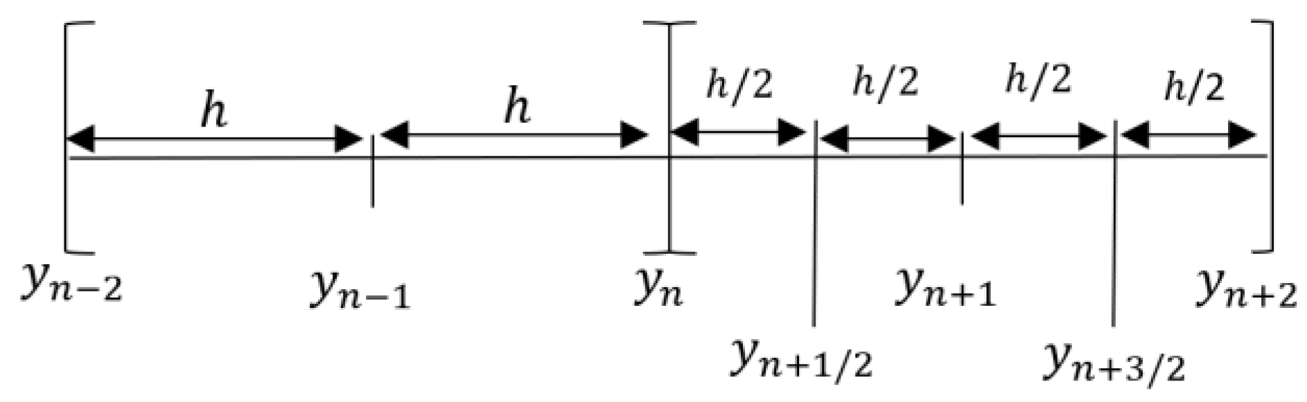
2. Derivation of BBDF with Off-Step Points, BBDFO

In this section, a detailed discussion of the derivation of the proposed method for the solution of Equation (1) will be presented. We considered the three points $y_{n-2}, y_{n-1,} y_n$ of equal step size h given by $h=x_{n+1}-x_n$ as the starting values and the two off-step points as $y_{n+1/2}$ and $y_{n+3/2}$ with half the step size, as illustrated in Figure 1.

In a 2-point block method (refer to Figure 1), the interval $\left[a,b\right]$ is divided into a series of blocks. In this case, the values at the points $y_{n-2}, y_{n-1,} y_n$ in the previous block are used to compute the solution of Equation (1) at $x_{n+1}$ and $x_{n+2}$ simultaneously. The class of methods we aim to consider is the general $k-$ step linear multistep method (LMM) in the form

$${\displaystyle \sum }_{j=0}^k{\alpha }_j{y}_{n+j}=h{\displaystyle \sum }_{j=0}^k{\beta }_j{f}_{n+j}$$

(2)

where $h$ is the step size, ${\alpha }_k=1, {\alpha }_{j }$ and ${\beta }_j$ are unknown constants which are uniquely determined and $k$ is the step number. Note that $y_{n+j}$ is the numerical solution for the exact solution $y\left(x_{n+j}\right)$, $f_{n+j}=f\left(x_{n+j}\right)$ and $n$ is the grid index.

In order to construct the new method, we need to extend the LMM in Equation (2) by introducing the off-step points. The extension of an LMM which involves $f\left(x,y\right)$ evaluated at an off-step point $\left(x_{n+r},y_{n+r}\right), 0<r<k, r\notin \left\{0,1,\dots ,k\right\}.$ that takes the following general form

$${\displaystyle \sum }_{j=0}^2{\alpha }_{j,i}{y}_{n+j-2}+{\displaystyle \sum }_{j=0}^3{\alpha }_{j+3,i}{y}_{n+\left(j+1\right)/2}=h{\beta }_i{f}_{n+i}$$

(3)

Equation (3) is expanded to generate the block method.

Therefore, the approximation at the point $x_{n+1}$ is given as follows

$${\alpha }_{0,i}{y}_{n-2}+{\alpha }_{1,i}{y}_{n-1}+{\alpha }_{2,i}{y}_n+{\alpha }_{3,i}{y}_{n+1/2}+{\alpha }_{4,i}{y}_{n+1}+{\alpha }_{5,i}{y}_{n+3/2}+{\alpha }_{6,i}{y}_{n+2}-h{\beta }_i{f}_{n+i}=0$$

(4)

To obtain the first formula for $y_{n+1/2}$, we substitute $i=1/2$ into Equation (4), and then, to remove the arbitrariness of the coefficients, we normalize the value of ${\alpha }_{3,1/2}=1$, which yields

$${\alpha }_{0,1/2}{y}_{n-2}+{\alpha }_{1,1/2}{y}_{n-1}+{\alpha }_{2,1/2}{y}_n+y_{n+1/2}+{\alpha }_{4,1/2}{y}_{n+1}+{\alpha }_{5,1/2}{y}_{n+3/2}+{\alpha }_{6,1/2}{y}_{n+2}-h{\beta }_{1/2}{f}_{n+1/2}=0$$

(5)

Equation (5) can also be interpreted as an exact relation between the approximated values of the equation by replacing the equation as follows

$$\begin{array}{c}{\alpha }_{0,1/2}y\left(x_n-2h\right)+{\alpha }_{1,1/2}y\left(x_n-h\right)+{\alpha }_{2,1/2}y\left(x_n\right)+y\left(x_n+\frac{1}{2}h\right)+{\alpha }_{4,1/2}y\left(x_n+h\right)\\ +{\alpha }_{5,1/2}y\left(x_n+\frac{3}{2}h\right)\\ +{\alpha }_{6,1/2}y\left(x_n+2h\right)-h{\beta }_{1/2}{y}^{\prime }\left(x_n+\frac{1}{2}h\right)=0\end{array}$$

(6)

The expansions of $y\left(x_n-2h\right),$ $y\left(x_n-h\right),$ $y\left(x_n\right),$ $y\left(x_n+\frac{1}{2}h\right),y\left(x_n+h\right),$ $y\left(x_n+\frac{3}{2}h\right),$ $y\left(x_n+2h\right)$ and $y^{\prime }\left(x_n+\frac{1}{2}h\right)$ using Taylor’s series about $x_n$ in Equation (6) are given below

$$\begin{array}{c}y\left(x_n-2h\right)=\left[y\left(x_n\right)-2y^{\prime }\left(x_n\right)+\frac{2^2}{2!}{y}^{″}\left(x_n\right)-\frac{2^3}{3!}{y}^{‴}\left(x_n\right)+\dots \right],\\ y\left(x_n-h\right)=\left[y\left(x_n\right)-y^{\prime }\left(x_n\right)+\frac{1^2}{2!}{y}^{″}\left(x_n\right)-\frac{1^3}{3!}{y}^{‴}\left(x_n\right)+\dots \right],\\ y\left(x_n\right)=\left[y\left(x_n\right)\right],\\ y\left(x_n+\frac{1}{2}h\right)=\left[y\left(x_n\right)+\frac{1}{2}{y}^{\prime }\left(x_n\right)+\frac{{\left(1/2\right)}^2}{2!}{y}^{″}\left(x_n\right)+\frac{{\left(1/2\right)}^3}{3!}{y}^{‴}\left(x_n\right)+\dots \right],\\ y\left(x_n+h\right)=\left[y\left(x_n\right)+y^{\prime }\left(x_n\right)+\frac{1^2}{2!}{y}^{″}\left(x_n\right)+\frac{1^3}{3!}{y}^{‴}\left(x_n\right)+\dots \right],\\ y\left(x_n+\frac{3}{2}h\right)=\left[y\left(x_n\right)+\frac{3}{2}{y}^{\prime }\left(x_n\right)+\frac{{\left(3/2\right)}^2}{2!}{y}^{″}\left(x_n\right)+\frac{{\left(3/2\right)}^3}{3!}{y}^{‴}\left(x_n\right)+\dots \right],\\ y\left(x_n+2h\right)=\left[y\left(x_n\right)+2y^{\prime }\left(x_n\right)+\frac{2^2}{2!}{y}^{″}\left(x_n\right)+\frac{2^3}{3!}{y}^{‴}\left(x_n\right)+\dots \right],\\ y^{\prime }\left(x_n+\frac{1}{2}h\right)=\left[y^{\prime }\left(x_n\right)+\frac{1}{2}{y}^{″}\left(x_n\right)+\frac{{\left(1/2\right)}^2}{2!}{y}^{‴}\left(x_n\right)+\frac{{\left(1/2\right)}^3}{3!}{y}^{\left(4\right)}\left(x_n\right)+\dots \right]\end{array}$$

(7)

By substituting Equation (7) into Equation (6), we obtain

$$\begin{array}{c}\begin{array}{ccc}\begin{array}{cc}& {\alpha }_{0,1/2}[y\left(x_n\right)-2y^{\prime }\left(x_n\right)+\frac{2^2}{2!}{y}^{″}\left(x_n\right)-\frac{2^3}{3!}{y}^{‴}\left(x_n\right)+\dots \left]+{\alpha }_{1,1/2}\right[y\left(x_n\right)-y^{\prime }\left(x_n\right)\end{array}& & \end{array}\\ \begin{array}{c}\begin{array}{cc}+& \frac{1^2}{2!}{y}^{″}\left(x_n\right)-\frac{1^3}{3!}{y}^{‴}\left(x_n\right)+\dots \left]+{\alpha }_{2,1/2}\right[y\left(x_n\right)]+[y\left(x_n\right)+\frac{1}{2}{y}^{\prime }\left(x_n\right)+\frac{{\left(1/2\right)}^2}{2!}{y}^{″}\left(x_n\right)\end{array}\end{array}\\ \begin{array}{c}\begin{array}{cc}+& \frac{{\left(1/2\right)}^3}{3!}{y}^{‴}\left(x_n\right)+\dots \left]+{\alpha }_{4,1/2}\right[y\left(x_n\right)+y^{\prime }\left(x_n\right)+\frac{1^2}{2!}{y}^{″}\left(x_n\right)+\frac{1^3}{3!}{y}^{‴}\left(x_n\right)+\dots ]\end{array}\end{array}\\ \begin{array}{c}\begin{array}{cc}+& {\alpha }_{5,1/2}[y\left(x_n\right)+\frac{3}{2}{y}^{\prime }\left(x_n\right)+\frac{{\left(3/2\right)}^2}{2!}{y}^{″}\left(x_n\right)+\frac{{\left(3/2\right)}^3}{3!}{y}^{‴}\left(x_n\right)+\dots \left]+{\alpha }_{6,1/2}\right[y\left(x_n\right)\end{array}\end{array}\\ \begin{array}{c}\begin{array}{cc}+& 2y^{\prime }\left(x_n\right)+\frac{2^2}{2!}{y}^{″}\left(x_n\right)+\frac{2^3}{3!}{y}^{‴}\left(x_n\right)+\dots \left]-h{\beta }_{1/2}\right[y^{\prime }\left(x_n\right)+\frac{1}{2}{y}^{″}\left(x_n\right)\end{array}\end{array}\\ \begin{array}{c}\begin{array}{cc}+& \frac{{\left(1/2\right)}^2}{2!}{y}^{‴}\left(x_n\right)+\frac{{\left(1/2\right)}^3}{3!}{y}^{\left(4\right)}\left(x_n\right)+\dots ]\\ & \end{array}=0\end{array}\end{array}$$

(8)

Next, we collect all the coefficients of $y\left(x_n\right),y^{\prime }\left(x_n\right),y^{″}\left(x_n\right),\dots$ in Equation (8) by factorizing. Then, $C_{p,i}$ is defined as the collected coefficients where $p=1, 2, 3, \dots$ and, as mentioned before, $i=1/2$, which yields

$$C_{0,1/2}y\left(x_n\right)+C_{1,1/2}h{y}^{\prime }\left(x_n\right)+C_{2,1/2}{h}^2{y}^{″}\left(x_n\right)+C_{3,1/2}{h}^3{y}^{‴}\left(x_n\right)\dots =0$$

(9)

where

$$\begin{array}{c}{C}_{0,1/2}={\alpha }_{0,1/2}+{\alpha }_{1,1/2}+{\alpha }_{2,1/2}+1+{\alpha }_{4,1/2}+{\alpha }_{5,1/2}+{\alpha }_{6,1/2}=0\\ C_{1,1/2}=-2{\alpha }_{0,1/2}-{\alpha }_{1,1/2}+\frac{1}{2}+{\alpha }_{4,1/2}+\frac{3}{2}{\alpha }_{5,1/2}+2{\alpha }_{6,1/2}-{\beta }_{,1/2}=0\\ C_{2,1/2}=\frac{{\left(2\right)}^2}{2!}{\alpha }_{0,1/2}+\frac{{\left(1\right)}^2}{2!}{\alpha }_{1,1/2}+\frac{{\left(1\right)}^2}{2!}+\frac{{\left(1\right)}^2}{2!}{\alpha }_{4,1/2}+\frac{{\left(3/2\right)}^2}{2!}{\alpha }_{5,1/2}+\frac{{\left(2\right)}^2}{2!}{\alpha }_{6,1/2}-\frac{{\left(1/2\right)}^1}{1!}{\beta }_{1/2}=0\\ C_{3,1/2}=-\frac{{\left(2\right)}^3}{3!}{\alpha }_{0,1/2}-\frac{{\left(1\right)}^3}{3!}{\alpha }_{1,1/2}+\frac{{\left(1/2\right)}^3}{3!}+\frac{{\left(1\right)}^3}{3!}{\alpha }_{4,1/2}+\frac{{\left(3/2\right)}^3}{3!}{\alpha }_{5,1/2}+\frac{{\left(2\right)}^3}{3!}{\alpha }_{6,1/2}-\frac{{\left(1/2\right)}^2}{2!}{\beta }_{1/2}=0\\ C_{4,1/2}=\frac{{\left(2\right)}^4}{4!}{\alpha }_{0,1/2}+\frac{{\left(1\right)}^4}{4!}{\alpha }_{1,1/2}+\frac{{\left(1/2\right)}^4}{4!}+\frac{{\left(1\right)}^4}{4!}{\alpha }_{4,1/2}+\frac{{\left(3/2\right)}^4}{4!}{\alpha }_{5,1/2}+\frac{{\left(2\right)}^4}{4!}{\alpha }_{6,1/2}-\frac{{\left(1/2\right)}^3}{3!}{\beta }_{1/2}=0\\ C_{5,1/2}=-\frac{{\left(2\right)}^5}{5!}{\alpha }_{0,1/2}-\frac{{\left(1\right)}^5}{5!}{\alpha }_{1,1/2}+\frac{{\left(1/2\right)}^5}{5!}+\frac{{\left(1\right)}^5}{5!}{\alpha }_{4,1/2}+\frac{{\left(3/2\right)}^5}{5!}{\alpha }_{5,1/2}+\frac{{\left(2\right)}^5}{5!}{\alpha }_{6,1/2}-\frac{{\left(1/2\right)}^4}{4!}{\beta }_{1/2}=0\\ C_{6,1/2}=\frac{{\left(2\right)}^6}{6!}{\alpha }_{0,1/2}+\frac{{\left(1\right)}^6}{6!}{\alpha }_{1,1/2}+\frac{{\left(1/2\right)}^6}{6!}+\frac{{\left(1\right)}^6}{6!}{\alpha }_{4,1/2}+\frac{{\left(3/2\right)}^6}{6!}{\alpha }_{5,1/2}+\frac{{\left(2\right)}^6}{6!}{\alpha }_{6,1/2}-\frac{{\left(1/2\right)}^5}{5!}{\beta }_{1/2}=0\end{array}$$

(10)

By solving Equation (9) simultaneously, the coefficients of the method are obtained.

$${\alpha }_{0,1/2}=\frac{1}{224}, {\alpha }_{1,1/2}=-\frac{5}{72}, {\alpha }_{2,1/2}=\frac{25}{16}, {\alpha }_{4,1/2}=-\frac{25}{8}, {\alpha }_{5,1/2}=\frac{5}{7}, {\alpha }_{6,1/2}=-\frac{25}{288} \mathrm{and} {\beta }_{1/2}=-\frac{5}{3}$$

By substituting all the values of ${\alpha }_s^{\prime }$ and ${\beta }_s^{\prime }$ obtained into Equation (5), we get

$$\frac{1}{224}{y}_{n-2}-\frac{5}{72}{y}_{n-1}+\frac{25}{16}{y}_n+y_{n+1/2}-\frac{25}{8}{y}_{n+1}+\frac{5}{7}{y}_{n+3/2}-\frac{25}{288}{y}_{n+2}+\frac{5}{3}h{f}_{n+1/2}=0$$

(11)

We rearrange Equation (11) to form the solution value of $y_{n+1/2}$,

$$y_{n+1/2}=-\frac{1}{224}{y}_{n-2}+\frac{5}{72}{y}_{n-1}-\frac{25}{16}{y}_n+\frac{25}{8}{y}_{n+1}-\frac{5}{7}{y}_{n+3/2}+\frac{25}{288}{y}_{n+2}-\frac{5}{3}h{f}_{n+1/2}.$$

Similarly, the procedures are repeated to obtain the next solution values by substituting $i=1$ and ${\alpha }_{4,1}=1$ for $y_{n+1}, i=3/2$ and ${\alpha }_{5,1}=1$ for $y_{n+3/2}$ and $i=2$ and ${\alpha }_{6,1}=1$ for $y_{n+2}$.

Hence, the BBDFO formulas are given by

$$\begin{array}{c}{y}_{n+1/2}=\frac{25}{288}{y}_{n+2}-\frac{5}{7}{y}_{n+3/2}+\frac{25}{8}{y}_{n+1}-\frac{25}{16}{y}_n+\frac{5}{72}{y}_{n-1}-\frac{1}{224}{y}_{n-2}-\frac{5}{3}h{f}_{n+1/2}\\ y_{n+1}=\frac{1}{10}{y}_{n+2}-\frac{192}{175}{y}_{n+3/2}+\frac{64}{25}{y}_{n+1/2}-\frac{3}{5}{y}_n+\frac{1}{25}{y}_{n-1}-\frac{1}{350}{y}_{n-2}+\frac{6}{5}h{f}_{n+1}\\ y_{n+3/2}=-\frac{1225}{7904}{y}_{n+2}+\frac{3675}{1976}{y}_{n+1}-\frac{245}{247}{y}_{n+1/2}+\frac{1225}{3952}{y}_n-\frac{49}{1976}{y}_{n-1}+\frac{15}{7904}{y}_{n-2}+\frac{105}{247}h{f}_{n+3/2}\\ y_{n+2}=\frac{1536}{665}{y}_{n+3/2}-\frac{48}{19}{y}_{n+1}+\frac{512}{285}{y}_{n+1/2}-\frac{12}{19}{y}_n+\frac{16}{285}{y}_{n-1}-\frac{3}{665}{y}_{n-2}+\frac{4}{19}h{f}_{n+2}\end{array}$$

(12)

In the following sections, the order, zero stability, region of stability and convergence of the new BBDFO method will be discussed.

3. Order, Convergence and Stability of the Method

This section is concerned with the order, convergence and stability of the proposed method. The following definitions, as stated in [6], give the meanings of order, consistency, zero stable and A-stability by relating them to the definition of convergence.

Definition 3.1.

(Convergence)

The necessary sufficient conditions for a linear multistep method to be convergent are that it must be consistent and zero-stable.

Definition 3.2.

(Order)

Linear multistep methods associated with the linear difference operator are said to be order $p$ if $C_1=C_2=\dots =C_p=0$ and $C_{p+1}\ne 0$.

Definition 3.3.

(Consistent)

The linear multistep method Equation (2) is said to be consistent if it has order $p\ge 1$.

Definition 3.4.

(Zero stable)

The linear multistep method Equation (2) is said to be zero stable if no root of the first characteristics of the polynomial has a modulus greater than one, and if every root with modulus one is simple.

Definition 3.5.

(A-stable)

If a method is stable for all $\lambda$ in the left-half plane $\left(Re\left(\lambda \right)\le 0\right)$, then the method is said to be A-stable. This means the stability region covers the entire negative left-half plane.

3.1. Order of the Method

The formula in Equation (12) can be rewritten as follows

$$\begin{array}{c}{y}_{n+1/2}-\frac{25}{288}{y}_{n+2}-\frac{5}{72}{y}_{n-1}+\frac{25}{16}{y}_n-\frac{25}{8}{y}_{n+1}+\frac{5}{7}{y}_{n+3/2}+\frac{1}{224}{y}_{n-2}=-\frac{5}{3}h{f}_{n+1/2}\\ y_{n+1}-\frac{1}{10}{y}_{n+2}+\frac{192}{175}{y}_{n+3/2}-\frac{64}{25}{y}_{n+1/2}+\frac{3}{5}{y}_n-\frac{1}{25}{y}_{n-1}+\frac{1}{350}{y}_{n-2}=\frac{6}{5}h{f}_{n+1}\\ y_{n+3/2}+\frac{1225}{7904}{y}_{n+2}-\frac{3675}{1976}{y}_{n+1}+\frac{245}{247}{y}_{n+1/2}-\frac{1225}{3952}{y}_n+\frac{49}{1976}{y}_{n-1}-\frac{15}{7904}{y}_{n-2}=\frac{105}{247}h{f}_{n+3/2}\\ y_{n+2}-\frac{1536}{665}{y}_{n+3/2}+\frac{48}{19}{y}_{n+1}-\frac{512}{285}{y}_{n+1/2}+\frac{12}{19}{y}_n-\frac{16}{285}{y}_{n-1}+\frac{3}{665}{y}_{n-2}=\frac{4}{19}h{f}_{n+2}\end{array}$$

(13)

We expressed Equation (13) by the following matrix form

$$\begin{array}{c}\left[\begin{array}{cccc}0& 0& 0& 1/224\\ 0& 0& 0& 1/350\\ 0& 0& 0& -15/7904\\ 0& 0& 0& 3/665\end{array}\right]\left[\begin{array}{c}{y}_{n-7/2}\\ y_{n-3}\\ y_{n-5/2}\\ y_{n-2}\end{array}\right]+\left[\begin{array}{cccc}0& -5/72& 0& 25/16\\ 0& -1/25& 0& 3/5\\ 0& 49/1976& 0& -1225/3952\\ 0& -16/285& 0& 12/19\end{array}\right]\left[\begin{array}{c}{y}_{n-3/2}\\ y_{n-1}\\ y_{n-1/2}\\ y_n\end{array}\right]\\ +\left[\begin{array}{cccc}1& -25/8& 5/7& -25/228\\ -64/25& 1& 192/175& -1/10\\ 245/247& -3675/1976& 1& 1225/7904\\ -512/285& 48/19& -1536/665& 1\end{array}\right]\left[\begin{array}{c}{y}_{n+1/2}\\ y_{n+1}\\ y_{n+3/2}\\ y_{n+2}\end{array}\right]\\ \begin{array}{c}=\left[\begin{array}{cccc}-5/3& 0& 0& 0\\ 0& 6/5& 0& 0\\ 0& 0& 105/247& 0\\ 0& 0& 0& 4/19\end{array}\right]\left[\begin{array}{c}h{f}_{n+1/2}\\ h{f}_{n+1}\\ h{f}_{n+3/2}\\ h{f}_{n+2}\end{array}\right].\end{array}\end{array}$$

Let

$$\begin{array}{c}{\alpha }_0=\left[\begin{array}{c}0\\ 0\\ 0\\ 0\end{array}\right],{\alpha }_1=\left[\begin{array}{c}0\\ 0\\ 0\\ 0\end{array}\right],{\alpha }_2=\left[\begin{array}{c}0\\ 0\\ 0\\ 0\end{array}\right],{\alpha }_3=\left[\begin{array}{c}1/224\\ 1/350\\ -15/7904\\ 3/665\end{array}\right],\\ {\alpha }_4=\left[\begin{array}{c}0\\ 0\\ 0\\ 0\end{array}\right],{\alpha }_5=\left[\begin{array}{c}-5/72\\ -1/25\\ 49/1976\\ -16/285\end{array}\right],{\alpha }_6=\left[\begin{array}{c}0\\ 0\\ 0\\ 0\end{array}\right],{\alpha }_7=\left[\begin{array}{c}25/16\\ 3/5\\ -1225/3952\\ 12/19\end{array}\right],\\ {\alpha }_8=\left[\begin{array}{c}1\\ -64/25\\ 245/247\\ -512/285\end{array}\right],{\alpha }_9=\left[\begin{array}{c}-25/8\\ 1\\ -3675/1976\\ 48/19\end{array}\right],{\alpha }_{10}=\left[\begin{array}{c}5/7\\ 192/175\\ 1\\ 1536/665\end{array}\right],{\alpha }_{11}=\left[\begin{array}{c}-25/288\\ -1/10\\ -1225/7904\\ 1\end{array}\right],\\ {\beta }_8=\left[\begin{array}{c}-5/3\\ 0\\ 0\\ 0\end{array}\right],{\beta }_9=\left[\begin{array}{c}0\\ 6/5\\ 0\\ 0\end{array}\right],{\beta }_{10}=\left[\begin{array}{c}0\\ 0\\ 105/247\\ 0\end{array}\right],{\beta }_{11}=\left[\begin{array}{c}0\\ 0\\ 0\\ 4/19\end{array}\right].\end{array}$$

By letting the collected terms of $y\left(x\right), y^{\prime }\left(x\right),y^{″}\left(x\right)$ in Equation (16) as $C_{p }$ where $p=0,1,2\dots ,$ we can determine the order of the method and the error constant of the method.

CThe associated linear difference operator, the order and error constants for the method in Equation (12), can be defined by extending the corresponding definitions for a linear multistep method.

$$ℒ\left[y\left(x\right);h\right]={\displaystyle \sum }_{j=0}^{11}\left[{\alpha }_{j}y\left(x+jh/2\right)-h{\beta }_j{y}^{\prime }\left(x+jh/2\right)\right]$$

(14)

Expanding on Equation (14) with Taylor’s series of expansions of $y\left(x+jh/2\right)$ and $y^{\prime }\left(x+jh/2\right)$ about $x,$ the terms can be collected to obtain

$$\begin{array}{c}L\left[y\left(x\right);h\right]={\displaystyle \sum }_{j=0}^{11}{\alpha }_j\left[y\left(x\right)+\frac{jh/2}{1!}{y}^{\prime }\left(x\right)+\frac{j{h}^2/2}{2!}{y}^{″}\left(x\right)+\frac{j{h}^3/2}{3!}{y}^{‴}\left(x\right)+\dots \right]\\ -{\displaystyle \sum }_{j=0}^{11}h{\beta }_j\left[y^{\prime }\left(x\right)+\frac{jh/2}{1!}{y}^{″}\left(x\right)+\frac{j{h}^2/2}{2!}{y}^{‴}\left(x\right)+\frac{j{h}^3/2}{3!}{y}^{\left(4\right)}\left(x\right)+\dots \right]\\ ={\displaystyle \sum }_{j=0}^{11}\left[{\alpha }_{j}y\left(x\right)\right]+\frac{1}{2}{\displaystyle \sum }_{j=0}^{11}\left[j{\alpha }_{j}y\left(x\right)-2{\beta }_j\right]h{y}^{\prime }\left(x\right)+\frac{1}{4}{\displaystyle \sum }_{j=0}^{11}\left[\frac{1}{2!}{j}^2{\alpha }_j-2j{\beta }_j\right]h^2{y}^{″}\left(x\right)\\ +\frac{1}{8}{\displaystyle \sum }_{j=0}^{11}\left[\frac{1}{3!}{j}^3{\alpha }_j-\frac{2}{2!}{j}^2{\beta }_j\right]h^3{y}^{‴}\left(x\right)+\dots \end{array}$$

(15)

We have

$$\begin{array}{l}{C}_0={\displaystyle {\displaystyle \sum }_{j=0}^{11}}{\alpha }_j=0\\ C_1={\displaystyle {\displaystyle \sum }_{j=0}^{11}}\left(j{\alpha }_j\right)-2{\displaystyle {\displaystyle \sum }_{j=0}^{11}}{\beta }_j=0\\ C_2={\displaystyle {\displaystyle \sum }_{j=0}^{11}}\frac{\left(j^2{\alpha }_j\right)}{2!}-2{\displaystyle {\displaystyle \sum }_{j=0}^{11}}\left(j{\beta }_j\right)=0\\ ⋮\\ C_6={\displaystyle {\displaystyle \sum }_{j=0}^{11}}\frac{\left(j^6{\alpha }_j\right)}{6!}-2{\displaystyle {\displaystyle \sum }_{j=0}^{11}}\frac{\left(j^5{\beta }_j\right)}{5!}=0\\ C_7={\displaystyle {\displaystyle \sum }_{j=0}^{11}}\frac{\left(j^7{\alpha }_j\right)}{7!}-2{\displaystyle {\displaystyle \sum }_{j=0}^{11}}\frac{\left(j^6{\beta }_j\right)}{6!}=\left[\begin{array}{c}\begin{array}{c}\begin{array}{c}-19280011/9072\\ 12256367/3150\end{array}\\ 3411415/1872\end{array}\\ -1204057/855\end{array}\right]\ne \left[\begin{array}{c}0\\ 0\\ 0\\ 0\end{array}\right].\end{array}$$

(16)

This yields the error constant

$$C_7=\left[\begin{array}{c}\begin{array}{c}\begin{array}{c}-19280011/9072\\ 12256367/3150\end{array}\\ 3411415/1872\end{array}\\ -1204057/855\end{array}\right]$$

which shows that the order of the method is six. Next, we examine the consistency of the method.

In accordance with Definition 3.3., the BBDFO(6) method is consistent since the order is greater than one.

3.2. Zero Stability of the Method

Next, we will discuss the zero stability of the method which is one of the criteria for the method to be convergent. The stability of the method in Equation (3) is determined using the linear test equation proposed by [27] as

$$y^{\prime }=\lambda y$$

(17)

where $\lambda$ is a complex constant with $\mathrm{Re}\left(\lambda \right)<0$. The substitution of Equation (17) into Equation (12) leads to the following

$$\begin{array}{c}{y}_{n+1/2}=\frac{25}{288}{y}_{n+2}-\frac{5}{7}{y}_{n+3/2}+\frac{25}{8}{y}_{n+1}-\frac{25}{16}{y}_n+\frac{5}{72}{y}_{n-1}-\frac{1}{224}{y}_{n-2}-\frac{5}{3}h\lambda y_{n+1/2}\\ y_{n+1}=\frac{1}{10}{y}_{n+2}-\frac{192}{175}{y}_{n+3/2}+\frac{64}{25}{y}_{n+1/2}-\frac{3}{5}{y}_n+\frac{1}{25}{y}_{n-1}-\frac{1}{350}{y}_{n-2}+\frac{6}{5}h\lambda y_{n+1}\\ y_{n+3/2}=-\frac{1225}{7904}{y}_{n+2}+\frac{3675}{1976}{y}_{n+1}-\frac{245}{247}{y}_{n+1/2}+\frac{1225}{3952}{y}_n-\frac{49}{1976}{y}_{n-1}+\frac{15}{7904}{y}_{n-2}+\frac{105}{247}h\lambda y_{n+3/2}\\ y_{n+2}=\frac{1536}{665}{y}_{n+3/2}-\frac{48}{19}{y}_{n+1}+\frac{512}{285}{y}_{n+1/2}-\frac{12}{19}{y}_n+\frac{16}{285}{y}_{n-1}-\frac{3}{665}{y}_{n-2}+\frac{4}{19}h\lambda y_{n+2}\end{array}$$

(18)

Equation (18) can be rewritten in the following matrix form

$$\begin{array}{c}\left[\begin{array}{cccc}1+\frac{5}{3}h\lambda & -25/8& 5/7& -25/228\\ -64/25& 1-\frac{6}{5}h\lambda & 192/175& -1/10\\ 245/247& -\frac{3675}{1976}& 1-\frac{105}{247}h\lambda & 1225/7904\\ -512/285& 48/19& -1536/665& 1-\frac{4}{19}h\lambda \end{array}\right]\left[\begin{array}{c}\begin{array}{l}{y}_{n+1/2}\end{array}\\ \begin{array}{l}{y}_{n+1}\end{array}\\ \begin{array}{l}{y}_{n+3/2}\end{array}\\ y_{n+2}\end{array}\right]\\ =\left[\begin{array}{cccc}0& 5/72& 0& -25/16\\ 0& 1/25& 0& -3/5\\ 0& -49/1976& 0& 1225/3952\\ 0& 16/285& 0& -12/19\end{array}\right]\left[\begin{array}{c}{y}_{n-3/2}\\ y_{n-1}\\ y_{n-1/2}\\ y_n\end{array}\right]+\left[\begin{array}{cccc}0& 0& 0& -1/224\\ 0& 0& 0& -1/350\\ 0& 0& 0& 15/7904\\ 0& 0& 0& -3/665\end{array}\right]\left[\begin{array}{c}{y}_{n-7/2}\\ y_{n-3}\\ y_{n-5/2}\\ y_{n-2}\end{array}\right],\end{array}$$

The matrices $A, B$ and $C$ are given by

$$\begin{gathered} \begin{array}{c}A=\left[\begin{array}{cccc}1+\frac{5}{3}h\lambda & -25/8& 5/7& -25/228\\ -64/25& 1-\frac{6}{5}h\lambda & 192/175& -1/10\\ 245/247& -\frac{3675}{1976}& 1-\frac{105}{247}h\lambda & 1225/7904\\ -512/285& 48/19& -1536/665& 1-\frac{4}{19}h\lambda \end{array}\right]\\ \end{array},B=\left[\begin{array}{cccc}0& 5/72& 0& -25/16\\ 0& 1/25& 0& -3/5\\ 0& -49/1976& 0& 1225/3952\\ 0& 16/285& 0& -12/19\end{array}\right] \\ C=\left[\begin{array}{cccc}0& 0& 0& -1/224\\ 0& 0& 0& -1/350\\ 0& 0& 0& 15/7904\\ 0& 0& 0& -3/665\end{array}\right] \end{gathered}$$

By inputting $H=h\lambda$, the stability polynomial $R\left(t,H\right)$ associated with the method in Equation (3) is determined by the location of the roots by solving the characteristic equation $\det \left(A{t}^2-Bt-C\right)=0$.

$$\begin{array}{c}R\left(t,H\right)=\det \left(A{t}^2-Bt-C\right)\\ =-\frac{5432344}{633555}{t}^8+\frac{199656}{23465}{t}^7+\frac{1544}{23465}{t}^6-\frac{56}{633555}{t}^5+\frac{225752}{23465}{t}^{8}H-\frac{112457}{23465}{t}^8{H}^2\\ +\frac{538504}{70395}{t}^{7}H+\frac{474}{361}{t}^8{H}^3+\frac{182023}{70395}{t}^7{H}^2-\frac{840}{4693}{t}^8{H}^4+\frac{2492}{4693}{t}^7{H}^3+\frac{664}{70395}{t}^{6}H \\ +\frac{49}{23465}{t}^6{H}^2+\frac{664}{70395}{t}^{6}H+\frac{49}{23465}{t}^6{H}^2+\frac{8}{211185}{t}^{5}H+\frac{18}{4693}{t}^6{H}^3+\frac{1}{70395}{t}^5{H}^2\end{array}$$

(19)

From the stability polynomial in Equation (19), it follows that its zero stability is determined by substituting $H=h\lambda =0$ into Equation (19), yielding

$$R\left(t,0\right)=-\frac{5432344}{633555}{t}^8+\frac{199656}{23465}{t}^7+\frac{1544}{23465}{t}^6-\frac{56}{633555}{t}^5$$

(20)

Solving $R\left(t,0\right)=0$, leads to the roots $t_1=t_2=t_3=t_4=t_5=0,t_6=0.0012,t_7=0.00719$ and $t_8=1$.

Since all the roots lie within $\left|t\right|\le 1$, we can conclude that the method for BBDFO(6) is zero stable. In the next subsection, we determine the absolute stability region for the BBDFO(6) method.

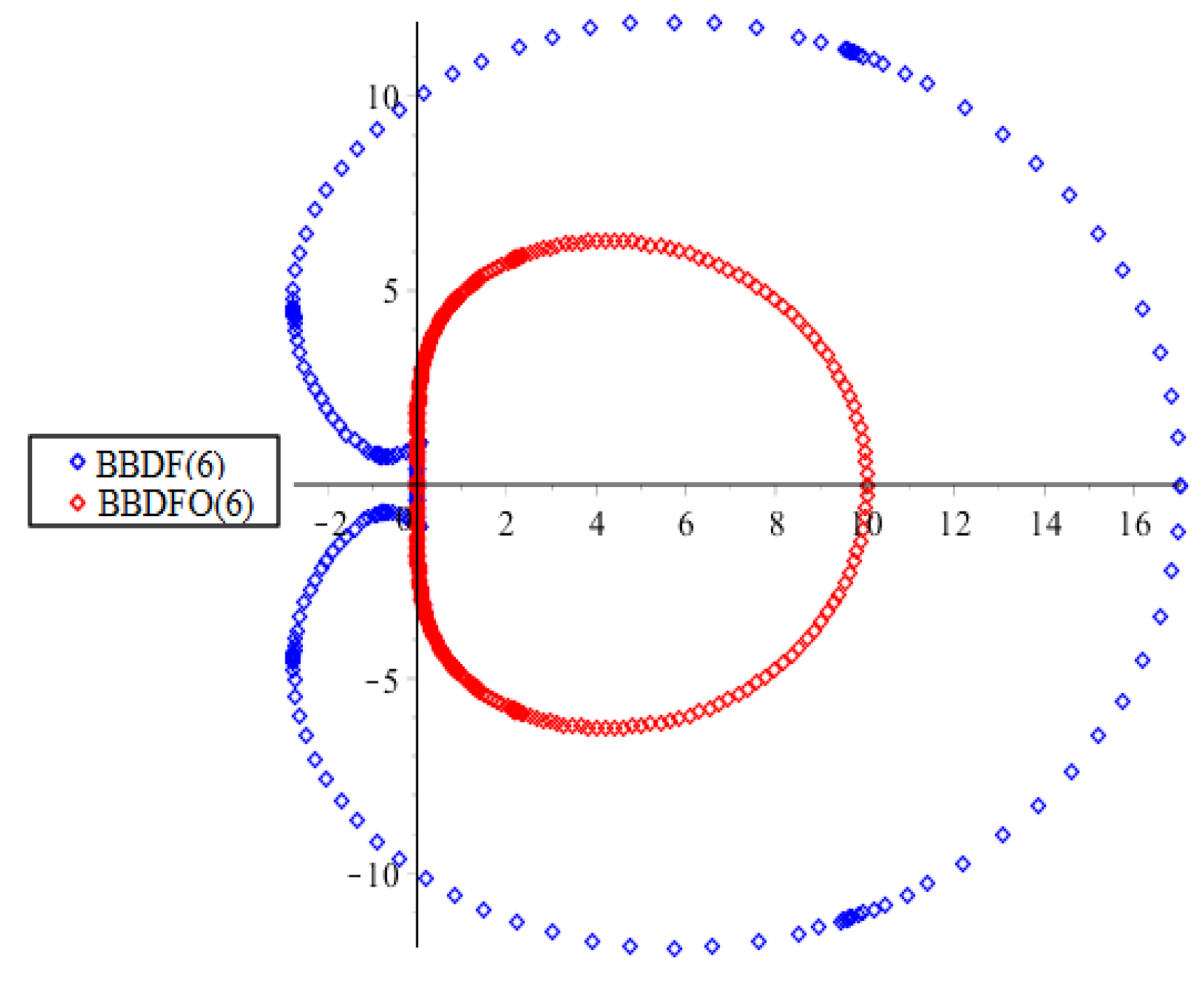
3.3. Stability Region of the Method

In this subsection, we plot the stability region of the method from the stability polynomial given in Equation (19). The boundary of the stability region is given by the set of points determined by $t=e^{i\theta }$, $0\le \theta \le 2\pi$. It is necessary to test the root condition ($\left|t\right|\le 1)$ of the stability polynomial at numerous grid points in the stability space to obtain the boundary of the stability region. The region of absolute stability for the method in Equation (12) is as shown in Figure 2.

Figure 2 shows the stability region which corresponds to the BBDFO(6) method. The stable region lies outside the closed region and it covers the entire left-half plane. From Definition 3.5, we can conclude that the BBDFO(6) method is A-stable.

3.4. Stability Comparison

The following figure shows the stability region of the new BBDFO(6) as compared to the existing stability region of the order six Block Backward Differentiation Formula without the off-step points, denoted as BBDF(6). For further discussion of the BBDF(6) method, see [28]. Figure 3 shows the region of both methods, i.e., the BBDFO(6) and the BBDF(6) in the complex $h\lambda$ plane.

Next, we compare the interval of instability of the new BBDFO(6) with the BBDF(6) by [28].

It is clear, from

Table 1. Comparison of instability interval BBDFO(6) versus BBDF(6).

Method	Interval of Instability
BBDFO(6)	(0, 10.05)
BBDF(6)	(0, 17.10)

, that the derived BBDFO(6) has a larger stability region.

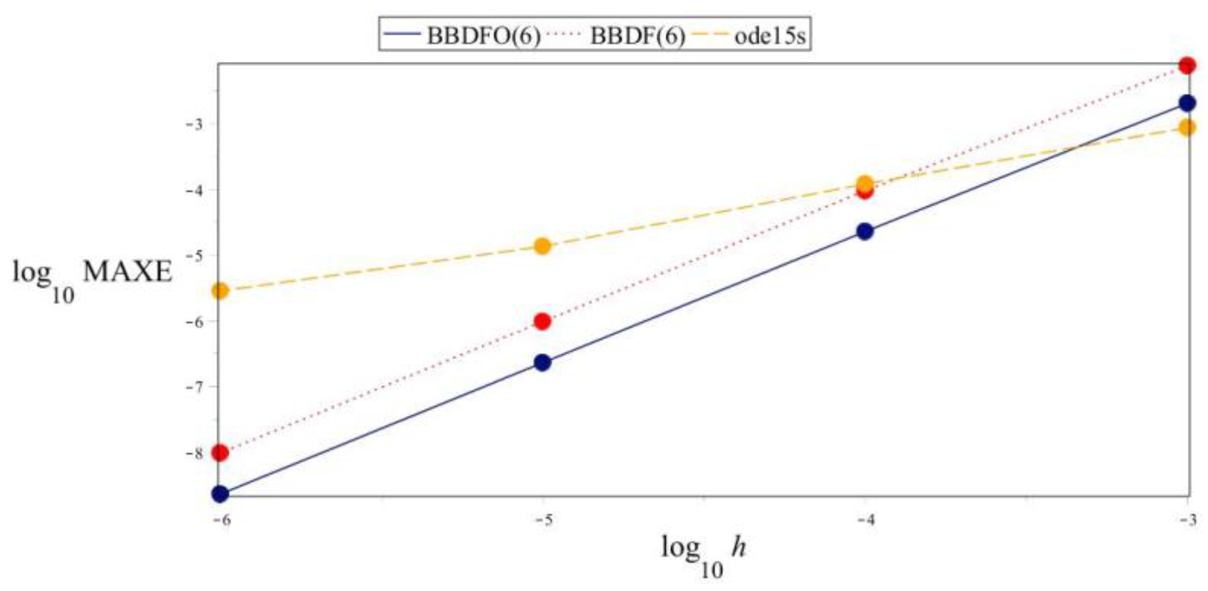
4. Numerical Results

In this section, the three problems that exhibit stiffness, given by $\lambda$, will be tested by using the proposed method with the step sizes $h={10}^{-3},{10}^{-4},{10}^{-5}$ and ${10}^{-6}.$ The efficiency of the method is compared to the exact solutions to illustrate the accuracy of the method.

Problem 1.

(See [29]).

$$\begin{gathered} y^{\prime }=-1000\left(y-1\right),y\left(0\right)=2,x\in \left[0,10\right]. \\ \lambda =-1000. \end{gathered}$$

Exact solution: $y\left(x\right)=e^{-1000x}+1$.

Problem 2.

(See [13]).

$$y^{\prime }=-y^3/2,y\left(0\right)=1,x\in \left[0,4\right].$$

Exact solution: $y\left(x\right)=1/\sqrt{1+x}.$

Problem 3.

(See [19]).

$$\begin{gathered} y_1^{\prime }=9y_1+24y_2+5\cos x-\frac{1}{3}\sin x,y_1\left(0\right)=4/3,x\in \left[0,10\right]. \\ {y}_2^{\prime }=-24y_1-51y_2-9\cos x+\frac{1}{3}\sin x,y_2\left(0\right)=2/3. \\ {\lambda }_1=-3,{\lambda }_2=-39. \end{gathered}$$

Exact solution:

$$\begin{gathered} y_1\left(x\right)=2e^{-3x}-e^{-39x}+\frac{1}{3}\cos x, \\ {y}_2\left(x\right)=-e^{-3x}+2e^{-39x}-\frac{1}{3}\cos x. \end{gathered}$$

For error calculations, the error formula is given by

$$\mathrm{MAXE}=\underset{0\le n\le NS}{\max }\left|y\left(x\right)-y_n\left(x\right)\right|$$

where $y\left(x_n\right)$ is the exact solution and $y_n$ is the computed solution.

The MATLAB solver ode15 s was chosen to compare the methods since it is the most popular code for solving stiff problems. It is a variable order solver which is based on the numerical differentiation formulas (NDFs) and optionally comes with the backward differentiation formulas (BDFs), also known as Gears’ method. The numerical results are presented in

Table 2. Numerical comparison for Problem 1.

$\mathit{h}.$	Methods	NS	MAXE
${10}^{-3}$	BBDFO(6)		2.11157($-$2)
	BBDF(6)		9.11882($-$4)
	ode15s		2.08844($-$3)
${10}^{-4}$	BBDFO(6)		5.54678($-$3)
	BBDF(6)		1.69293($-$2)
	ode15s		2.60950($-$4)
${10}^{-5}$	BBDFO(6)		7.38966($-$5)
	BBDF(6)		3.02723($-$4)
	ode15s		3.76862($-$5)
${10}^{-6}$	BBDFO(6)		7.60256($-$7)
	BBDF(6)		3.20426($-$6)
	ode15s		6.32160($-$6)

,

Table 3. Numerical comparison for Problem 2.

$\mathit{h}.$	Methods	NS	MAXE
${10}^{-3}$	BBDFO(6)		5.68483($-$7)
	BBDF(6)		2.38845($-$6)
	ode15s		9.37878($-$4)
${10}^{-4}$	BBDFO(6)		5.71640($-$9)
	BBDF(6)		2.41537($-$8)
	ode15s		1.14126($-$4)
${10}^{-5}$	BBDFO(6)		5.71960($-$11)
	BBDF(6)		2.41808($-$10)
	ode15s		1.75037($-$5)
${10}^{-6}$	BBDFO(6)		9.52614($-$11)
	BBDF(6)		7.40070($-$11)
	ode15s		2.61573($-$6)

and

Table 4. Numerical comparison for Problem 3.

$\mathit{h}.$	Methods	NS	MAXE
${10}^{-3}$	BBDFO(6)		2.04408($-$3)
	BBDF(6)		7.62867($-$3)
	ode15s		8.69860($-$4)
${10}^{-4}$	BBDFO(6)		2.28504($-$5)
	BBDF(6)		9.54280($-$5)
	ode15s		1.21447($-$4)
${10}^{-5}$	BBDFO(6)		2.31054($-$7)
	BBDF(6)		9.75695($-$7)
	ode15s		1.36101($-$5)
${10}^{-6}$	BBDFO(6)		2.31311($-$9)
	BBDF(6)		9.77861($-$9)
	ode15s		2.85643($-$6)

.

Figure 4, Figure 5 and Figure 6 are the graphs showing the accuracy of the BBDFO(6) compared with the BBDF(6) and the ode15 s at different time steps, h.

As seen in Figure 4, Figure 5 and Figure 6, the global errors produced by the BBDFO(6) are smaller global errors compared with the BBDF(6) and the ode15 s as the value of h becomes smaller.

5. Conclusions

In conclusion, a new method with off-step points, the BBDFO of order six, is introduced as the numerical solution of stiff initial-value problems. The stability analysis of the BBDFO indicates that the method is consistent and zero stable; therefore, the BBDFO(6) is convergent. The developed method is suitable to solve stiff ODEs since it possesses an A-stability property. The interval of instability for the BBDFO(6) is smaller than that of the BBDF(6) proposed by [28]. The numerical results obtained using the BBDFO(6) were compared with existing methods of a similar type and performed with the MATLAB solver ode15s. The BBDFO(6) is found to be more efficient at certain step sizes. Hence, we can conclude that the BBDFO(6) could be a compatible alternative solver for stiff ODEs.

References

1. Henrici, P. Discrete Variable Methods in Ordinary Differential Equations; John Wiley & Sons Inc.: Hoboken, NJ, USA, 1969. [Google Scholar]
2. Curtiss, C.F.; Hirschfelder, J.O. Integration of stiff equations. Proc. Natl. Acad. Sci. USA 1952, 38, 235–243. [Google Scholar] [CrossRef] [PubMed] [Green Version]
3. Lambert, J.D. Numerical Methods for Ordinary Differential Systems: The Initial Value Problem; John Wiley & Sons, Inc.: Hoboken, NJ, USA, 1991. [Google Scholar]
4. Wanner, G.; Hairer, E. Solving Ordinary Differential Equations II; Springer: Berlin/Heidelberg, Germany, 1996; p. 2. [Google Scholar]
5. Butcher, J.C. Numerical Methods for Ordinary Differential Equations; John Wiley & Sons: Hoboken, NJ, USA, 2016. [Google Scholar]
6. Lambert, J.D. Computational Methods in Ordinary Differential Equations; John Wiley & Sons: Hoboken, NJ, USA, 1973; pp. 22–23, 231–233. [Google Scholar]
7. Gear, C.W. Numerical Initial Value Problems in Ordinary Differential Equations; Prentice-Hall: Englewood Cliffs, NJ, USA, 1971; ISBN 013-626606-1. [Google Scholar]
8. Rosser, J.B. A Runge-Kutta for all seasons. Siam Rev. 1967, 9, 417–452. [Google Scholar] [CrossRef]
9. Shampine, L.F.; Watts, H.A. Block implicit one-step methods. Math. Comput. 1969, 23, 731–740. [Google Scholar] [CrossRef]
10. Majid, Z.A.; Suleiman, M.B.; Omar, Z. 3-point implicit block method for solving ordinary differential equations. Bull. Malays. Math. Sci. Soc. Second Ser. 2006, 29, 23–31. [Google Scholar]
11. Ibrahim, Z.B.; Othman, K.I.; Suleiman, M. Implicit r-point block backward differentiation formula for solving first-order stiff ODEs. Appl. Math. Comput. 2007, 186, 558–565. [Google Scholar] [CrossRef]
12. Ibrahim, Z.B.; Othman, K.I.; Suleiman, M. 2-point block predictor-corrector of backward differentiation formulas for solving second order ordinary differential equations directly. Chiang Mai J. Sci. 2012, 39, 502–510. [Google Scholar]
13. Musa, H.; Suleiman, M.B.; Senu, N. Fully implicit 3-point block extended backward differentiation formula for stiff initial value problems. Appl. Math. Sci. 2012, 6, 4211–4228. [Google Scholar]
14. Nasir, N.A.A.M.; Ibrahim, Z.B.; Othman, K.I.; Suleiman, M. Numerical solution of first order stiff ordinary differential equations using fifth order block backward differentiation formulas. Sains Malays. 2012, 41, 489–492. [Google Scholar]
15. Musa, H.; Suleiman, M.B.; Ismail, F.; Senu, N.; Ibrahim, Z.B. An improved 2–point block backward differentiation formula for solving stiff initial value problems. Aip. Conf. Proc. Am. Inst. Phys. 2013, 1522, 211–220. [Google Scholar]
16. Jator, S.N.; Agyingi, E. Block Hybrid-Step Backward Differentiation Formulas for Large Stiff Systems. Int. J. Comput. Math. 2014, 2014, 1–8. [Google Scholar] [CrossRef] [Green Version]
17. Jana Aksah, S.; Ibrahim, Z.B.; Zawawi, M.; Shah, I. Stability analysis of singly diagonally implicit block backward differentiation formulas for stiff ordinary differential equations. Mathematics 2019, 7, 211. [Google Scholar] [CrossRef] [Green Version]
18. Ola Fatunla, S. Block methods for second order ODEs. Int. J. Comput. Math. 1991, 41, 55–63. [Google Scholar] [CrossRef]
19. Ibrahim, Z.B. Block Multistep Methods for Solving Ordinary Differential Equations. Ph.D. Thesis, Universiti Putra Malaysia, Putrajaya, Malaysia, 2006. [Google Scholar]
20. Musa, H.; Suleiman, M.B.; Ismail, F.; Senu, N.; Ibrahim, Z.B. An accurate block solver for stiff IVPs. ISRN Appl. Math. 2013, 7, 61–67. [Google Scholar]
21. Abasi, N.; Suleiman, M.; Abasi, N.; Musa, H. 2-point block BDF method with off-step points for solving stiff ODEs. J. Soft Comput. Appl. 2014, 1–15. [Google Scholar] [CrossRef] [Green Version]
22. Yap, L.K.; Ismail, F. Block Methods with Off-Steps Points for Solving First Order Ordinary Differential Equations. In International Conference on Mathematical Sciences and Statistics 2013; Springer: Singapore, 2013; pp. 275–284. [Google Scholar]
23. Babangida, B.; Musa, H. Diagonally Implicit Super Class of Block Backward Differentiation Formula with Off-Step Points for Solving Stiff Initial Value Problems. J. Appl. Comput. Math. 2016, 5, 1–7. [Google Scholar]
24. Ra’ft Abdelrahim, Z.O.; Kuboye, J.O. New Hybrid Block Method with Three Off-Step Points for Solving First Order Ordinary Differential Equations. Am. J. Appl. Sci. 2016, 13, 209–212. [Google Scholar] [CrossRef]
25. Ajileye, G.; Amoo, S.A.; Ogwumu, O.D. Hybrid Block Method Algorithms for Solution of First Order Initial Value Problems in Ordinary Differential Equations. J. Appl. Comput. Math. 2019, 7, 2. [Google Scholar]
26. Agarwal, P.; Ibrahim, I.H. A new type OF hybrid multistep multiderivative formula for solving stiff IVPs. Adv. Differ. Equ. 2019, 2019, 1–14. [Google Scholar] [CrossRef] [Green Version]
27. Dahlquist, G.G. A special stability problem for linear multistep methods. BIT Numer. Math. 1963, 3, 27–43. [Google Scholar] [CrossRef]
28. Nasir, N.A.A.M. Parallel Multiblock Backward Differentiation Formulae for Solving First Order Ordinary Differential Equations. Master’s Thesis, Universiti Putra Malaysia, Putrajaya, Malaysia, 2012. [Google Scholar]
29. Othman, K.I.; Ibrahim, Z.B.; Suleiman, M.; Majid, Z. Automatic intervalwise block partitioning using Adams type method and backward differentiation formula for solving ODEs. Appl. Math. Comput. 2007, 188, 1642–1646. [Google Scholar] [CrossRef]
Figure 1. Block method with off-step points.
Symmetry 12 00952 g001
Figure 2. Stability region of the sixth order Block Backward Differentiation Formula with two off-step points (BBDFO(6)).
Symmetry 12 00952 g002
Figure 3. Comparison of the stability regions between the BBDFO(6) and the Block Backward Differentiation Formula without the off-step points (BBDF(6)).
Symmetry 12 00952 g003
Figure 4. Graph of log 10 MAXE versus log 10 h for Problem 1.
Symmetry 12 00952 g004
Figure 5. Graph of log 10 MAXE versus log 10 h for Problem 2.
Symmetry 12 00952 g005
Figure 6. Graph of log 10 MAXE versus log 10 h for Problem 3.
Symmetry 12 00952 g006