Subclasses of Starlike and Convex Functions Associated with the Limaçon Domain

Abstract

Let ${\mathcal{ST}}_L\left(s\right)$ and ${\mathcal{CV}}_L\left(s\right)$ denote the family of analytic and normalized functions f in the unit disk $\mathbb{D}:=\left\{z:\left|z\right|<1\right\}$, such that the quantity $z{f}^{\prime }\left(z\right)/f\left(z\right)$ or $1+z{f}^{″}\left(z\right)/f^{\prime }\left(z\right)$ respectively are lying in the region bounded by the limaçon ${\left[{(u-1)}^2+v^2-s^4\right]}^2=4s^2\left[{\left(u-1+s^2\right)}^2+v^2\right],$ where $0<s\le 1/\sqrt{2}$. The limaçon of Pascal is a curve that possesses properties which qualify it for the several applications in mathematics, statistics (hypothesis testing problem) but also in mechanics (fluid processing applications, known limaçon technology is employed to extract electrical power from low-grade heat, etc.). In this paper we present some results concerning the behavior of f on the classes ${\mathcal{ST}}_L\left(s\right)$ or ${\mathcal{CV}}_L\left(s\right)$. Some appropriate examples are given.

1. An Analytic Representation of a Limaçon of Pascal

A limaçon, known also as a limaçon of Pascal is a curve that in polar coordinates has the form

$$r=b+acos\theta ,$$

(1)

where $a,b$ are positive real numbers and $\theta \in \langle 0,2\pi )$. This is also called the limaçon of Pascal. The word “limaçon” comes from the Latin “limax”, meaning “snail”. Converting to Cartesian coordinates the Equation (1) becomes

$${\left(x^2+y^2-ax\right)}^2=b^2\left(x^2+y^2\right),$$

that has the following parametric form

$$\begin{array}{ccc}x\hfill & =& (b+acos\theta )cos\theta ,\\ y\hfill & =& (b+acos\theta )sin\theta .\end{array}$$

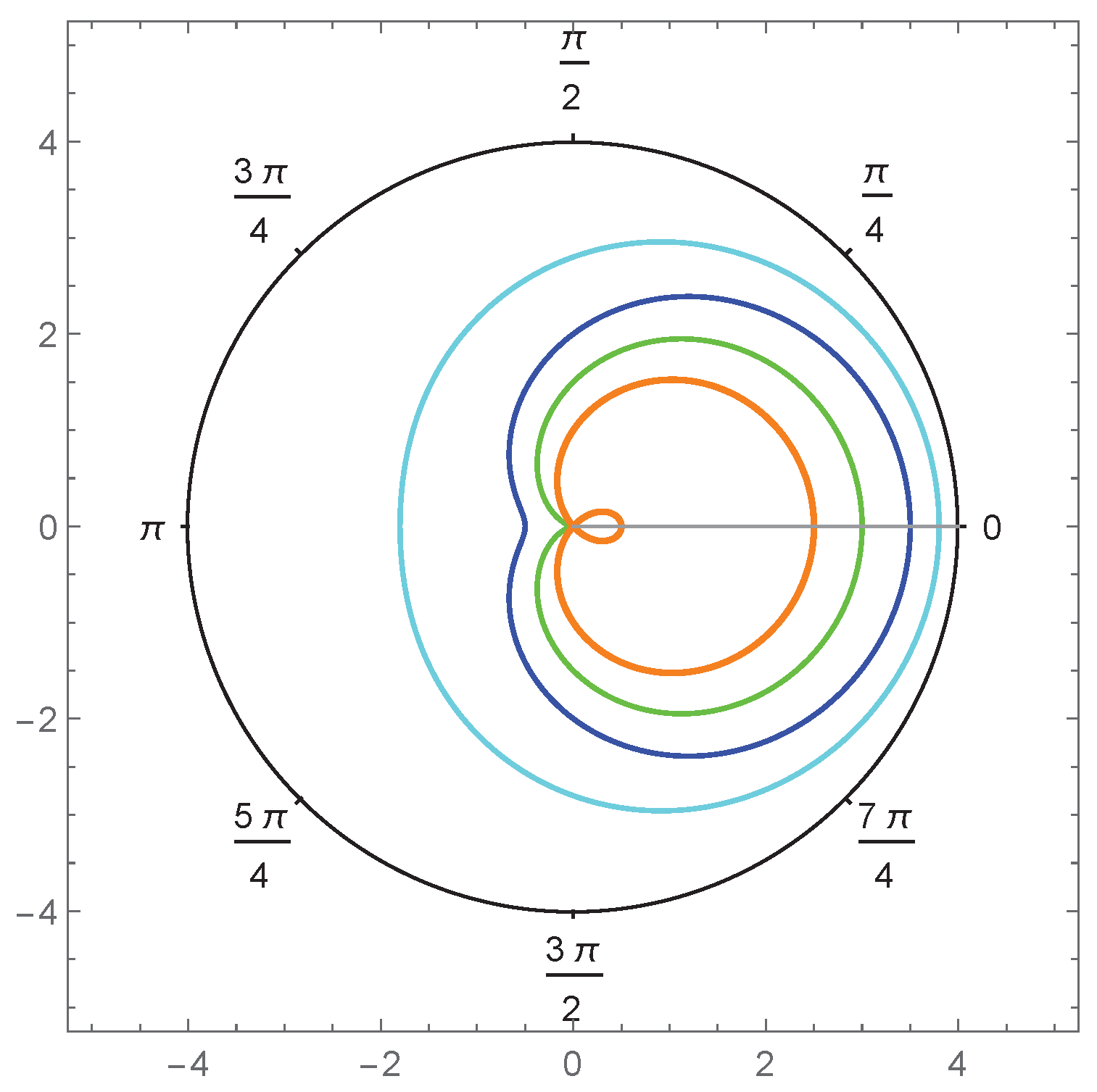
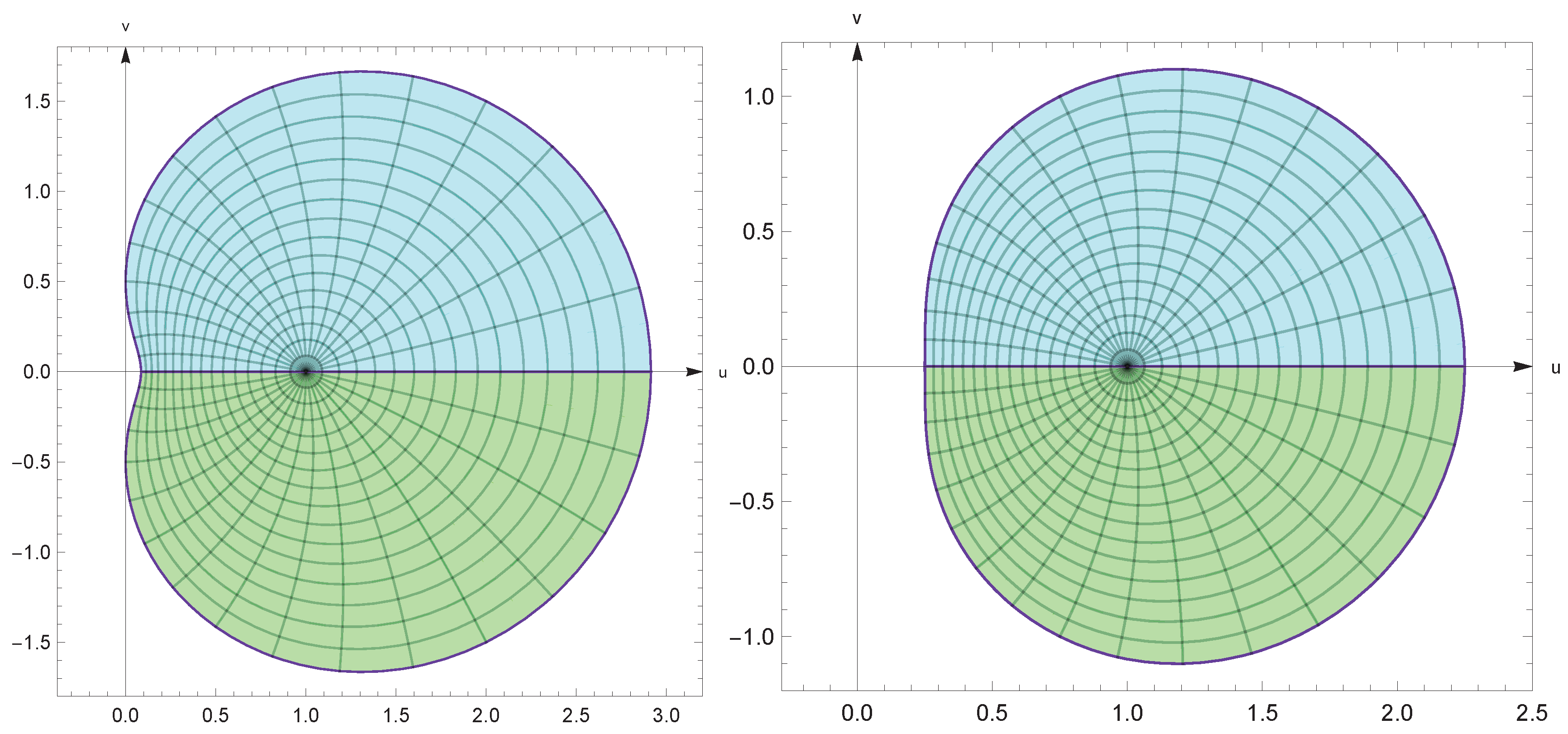
If $b\ge 2a$, a limaçon is convex, and if $2a>b>a$ has an indentation bounded by two inflection points. If $b=a$, the limaçon degenerates to a cardioid. If $b<a$, the limaçon has an inner loop, and when $b=a/2$, it is a trisectrix (but not the Maclaurin trisectrix). In Figure 1, we have plotted the limaçon $r=b+acos\theta$ for some different values of a and b.

An analytic description of a limaçon is given by

$${\mathbb{L}}_s\left(z\right)={\left(1+sz\right)}^2,$$

(2)

that maps the unit disk $\mathbb{D}=\left\{z\in \mathbb{C}:\left|z\right|<1\right\}$ of the complex plane $\mathbb{C}$, onto a domain bounded by a limaçon defined by

$$\partial \mathfrak{D}\left(s\right)=\left\{u+iv\in \mathbb{C}:{\left[{(u-1)}^2+v^2-s^4\right]}^2=4s^2\left[{\left(u-1+s^2\right)}^2+v^2\right]\right\},$$

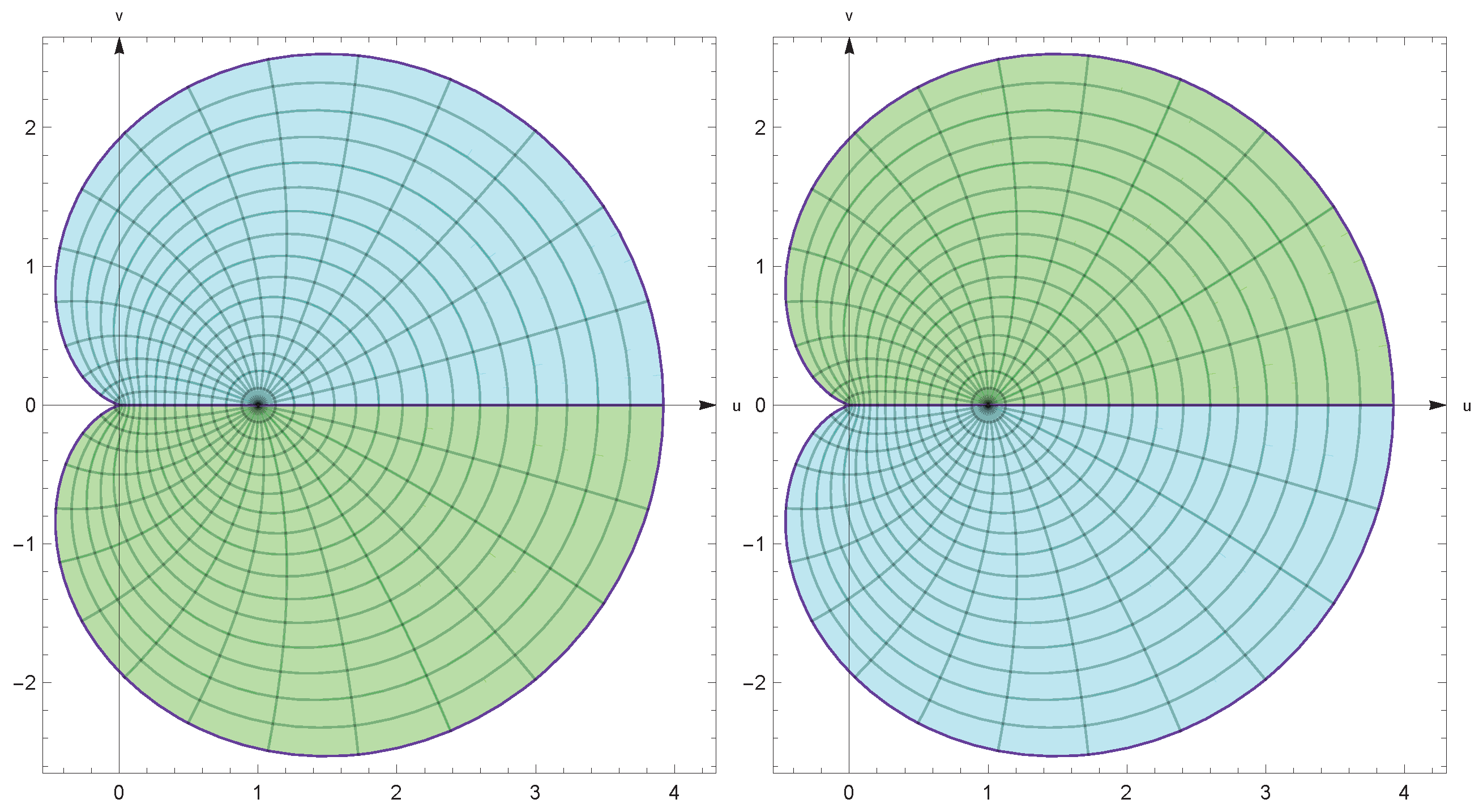
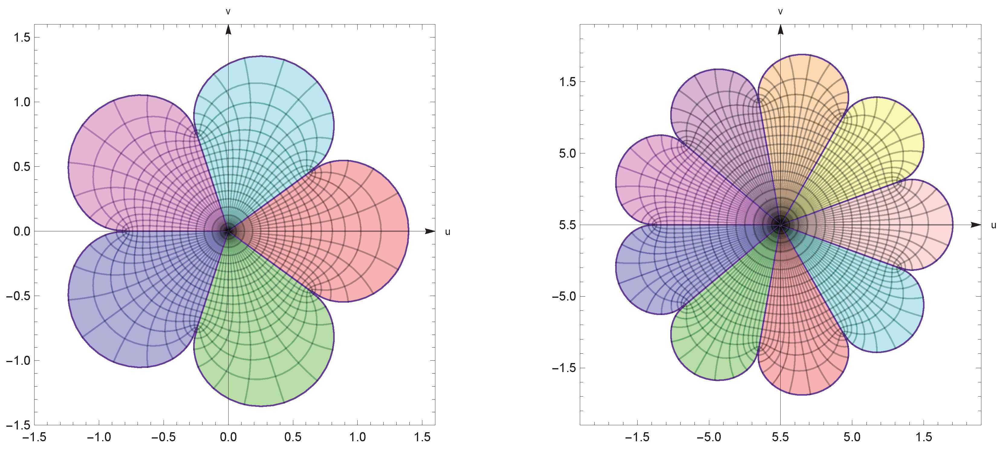
where $s\in \langle -1,1\rangle \backslash \left\{0\right\}$ (The Figure 2 shows an example of a image of $\mathbb{D}$ by the function ${\mathbb{L}}_s$ for different values of s). Indeed, setting $z=e^{i\theta }$ with $0\le \theta <2\pi$, we obtain

$$\begin{array}{c}\hfill {\mathbb{L}}_s\left(e^{i\theta }\right)={\left(1+s{e}^{i\theta }\right)}^2=(1+2scos\theta +s^{2}cos2\theta )+i(2ssin\theta +s^{2}sin2\theta )\end{array}$$

(3)

Let us denote $u=u\left(\theta \right)=\Re \left\{{\mathbb{L}}_s\left(e^{i\theta }\right)\right\}$ and $v=v\left(\theta \right)=\Im \left\{{\mathbb{L}}_s\left(e^{i\theta }\right)\right\}$. Then

$$u=1+2scos\theta +s^{2}cos2\theta ,v=2ssin\theta +s^{2}sin2\theta$$

(4)

Taking a parametrization

$$\frac{u-1+s^2}{2s}=(1+scos\theta )cos\theta ,\frac{v}{2s}=(1+scos\theta )sin\theta ,$$

we can find that the image of unit circle $\left|z\right|=1$ under ${\mathbb{L}}_s(·)$ is a curve given by

$${\left[{(u-1)}^2+v^2-s^4\right]}^2=4s^2\left[{\left(u-1+s^2\right)}^2+v^2\right],$$

that is the limaçon of Pascal. Furthermore, ${\mathbb{L}}_s$ is an analytic and does not have any poles in $\overline{\mathbb{D}}$ since $s\in [-1,1]\backslash \left\{0\right\}$.

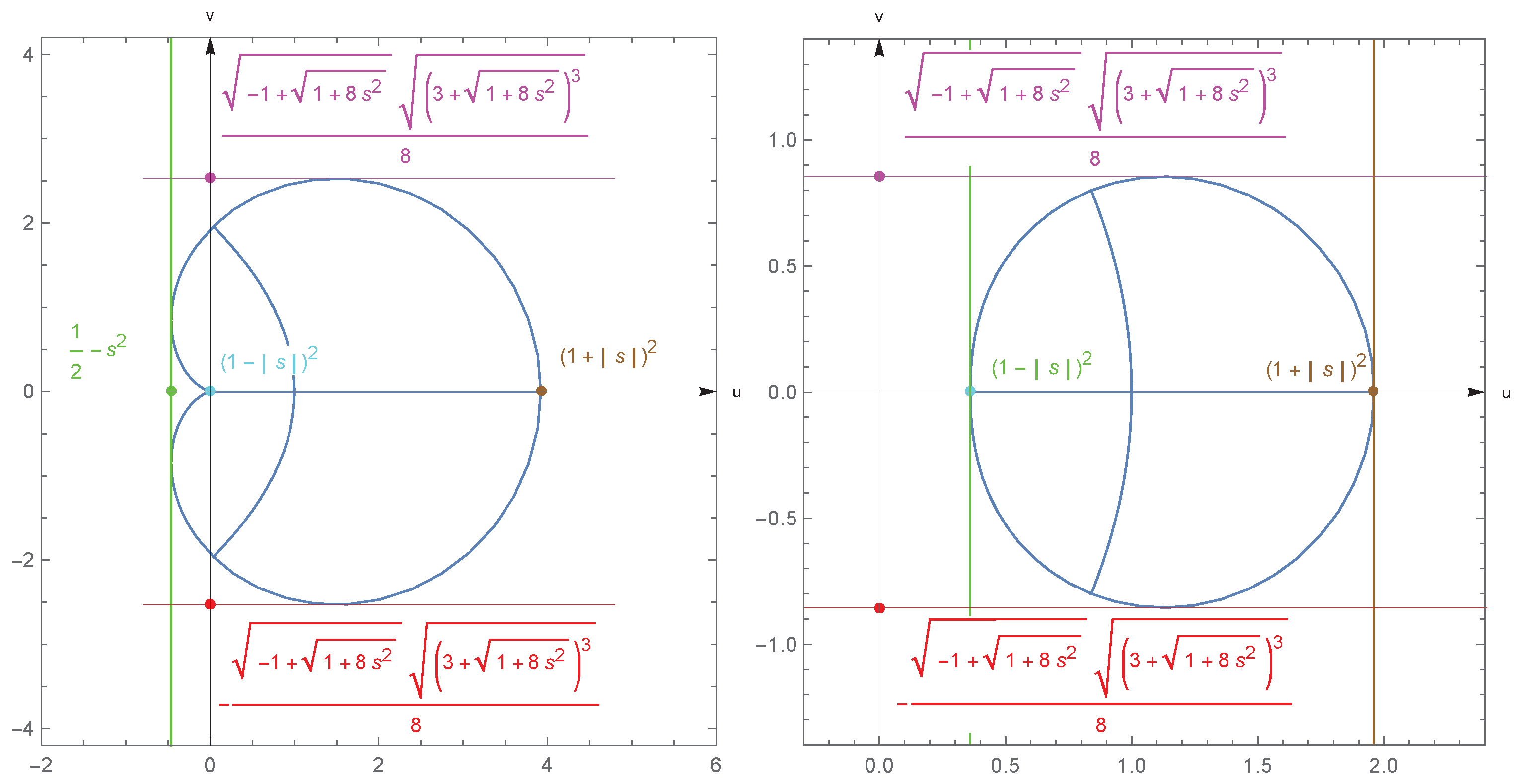
It is easy to check that the real and an imaginary part of ${\mathbb{L}}_s\left(e^{i\theta }\right)$ is bounded. Then $\Re \left\{{\mathbb{L}}_s(\mathbb{D}\right\}$ and $\Im \left\{{\mathbb{L}}_s\left(\mathbb{D}\right)\right\}$ attains its minimum and maximum on $\partial \mathbb{D}$. Indeed, by Equation (4) we have

$$\Re \left\{{\mathbb{L}}_s\left({\mathrm{e}}^{i\theta }\right)\right\}=1-s^2+2scos\theta +2s^2{cos}^2\theta =:g\left(\theta \right).$$

(5)

The extremum of $g\left(\theta \right)$ is attained at the critical points of the above function, equivalently

$$-2s(1+2scos\theta )sin\theta =0.$$

which are $\theta =0,\theta =\pi$ and the solution of equation $cos\theta =-1/\left(2s\right)$, if $\left|s\right|\ge 1/2$. Clearly, the minimum value is when $cos\theta =-1/\left(2s\right)$ and the maximum value is when $\theta =0$ or $\theta =\pi$. Thus,

$$\frac{1}{2}-s^2\le \Re \left\{{\mathbb{L}}_s\left({\mathrm{e}}^{i\theta }\right)\right\}\le {\left(1+\left|s\right|\right)}^2.$$

For $\left|s\right|>1/2$ the critical points are $\theta =0$ and $\theta =\pi$. Thus we have

$${(1-|s\left|\right)}^2\le \Re \left\{{\mathbb{L}}_s\left({\mathrm{e}}^{i\theta }\right)\right\}\le {\left(1+\left|s\right|\right)}^2.$$

In addition, from Equation (4) we have

$$\Im \left\{{\mathbb{L}}_s\left({\mathrm{e}}^{i\theta }\right)\right\}=2ssin\theta +s^{2}sin2\theta =:F\left(\theta \right).$$

Then $F^{\prime }\left(\theta \right)=2s(s{cos}^2\theta +cos\theta -s)=0$ if and only if

$$cos{\theta }_{1,2}=\frac{-1\pm \sqrt{1+8s^2}}{4s},$$

$|cos{\theta }_1|=|(-1+\sqrt{1+8s^2})/\left(4s\right)|\le 1$ for $s\in [-1,1]\backslash \left\{0\right\}$. Using an elementary computation we can find then that

$$\left|\Im \left\{{\mathbb{L}}_s\left({\mathrm{e}}^{i\theta }\right)\right\}\right|\le \frac{{\left(3+\sqrt{1+8s^2}\right)}^{3/2}{\left(-1+\sqrt{1+8s^2}\right)}^{1/2}}{8}.$$

The above discussion can be summarized as follows (cf. Figure 3).

Theorem 1.

Let ${\mathbb{L}}_s(·)$ be a function defined by Equation (6) with $s\in [-1,1]\backslash \left\{0\right\}$. Then

$$\underset{z\in \mathbb{D}}{max}\Re \left\{{\mathbb{L}}_s\left(z\right)\right\}={(1+|s\left|\right)}^2$$

$$\underset{z\in \mathbb{D}}{min}\Re \left\{{\mathbb{L}}_s\left(z\right)\right\}=m_0\left(s\right)=\left\{\begin{array}{cc}{\displaystyle \frac{1}{2}}-s^2\hfill & \mathit{for}\left|s\right|\ge {\displaystyle \frac{1}{2}},\hfill \\ {(1-|s\left|\right)}^2\hfill & \mathit{for}0<\left|s\right|\le {\displaystyle \frac{1}{2}}.\hfill \end{array}\right.$$

$$\left|\Im \left\{{\mathbb{L}}_s\left(z\right)\right\}\right|<\frac{{\left(3+\sqrt{1+8s^2}\right)}^{3/2}{\left(-1+\sqrt{1+8s^2}\right)}^{1/2}}{8}\mathit{for}z\in \mathbb{D}.$$

$${\mathbb{L}}_s\left(\mathbb{D}\right)=\mathfrak{D}\left(s\right)=\left\{u+iv:{\left[{(u-1)}^2+v^2-s^4\right]}^2<4s^2\left[{\left(u-1+s^2\right)}^2+v^2\right]\right\}.$$

2. Definitions and Preliminaries

Let $\mathcal{A}$ denote the class of functions $f\left(z\right)$ of the form:

$$f\left(z\right)=z+\sum _{n=2}^{\infty }{a}_n{z}^n\mathit{for}z\in \mathbb{D},$$

(6)

which are analytic in the open unit disk $\mathbb{D}:=\left\{z\in \mathbb{C}:\left|z\right|<1\right\}$ in the complex plane $\mathbb{C}$. The subclass of $\mathcal{A}$ consisting of all univalent functions f in $\mathbb{D}$, is denoted by $\mathcal{S}$. A functions $f\in \mathcal{S}$ is said to belong to the class $\mathcal{ST}\left(\beta \right)$, called starlike functions of order $0\le \beta <1$, if $\Re \left\{z{f}^{\prime }\left(z\right)/f\left(z\right)\right\}>\beta ,$ and is said to belong to the class $\mathcal{CV}\left(\beta \right)$, called convex functions of order $0\le \beta <1$, if $\Re \{1+z{f}^{″}\left(z\right)/f^{\prime }\left(z\right)\}>\beta$ [1].

The special cases occur for $\beta =0$, and then we get the classical classes of starlike and convex univalent functions, denoted $\mathcal{ST}:=\mathcal{ST}\left(0\right)$ and $\mathcal{CV}:=\mathcal{CV}\left(0\right)$, respectively. Let f and g be analytic in $\mathbb{D}$. Then the function f is said to subordinate to g in $\mathbb{D}$ written by $f\left(z\right)\prec g\left(z\right)$, if there exists a self-map function $\omega \left(z\right)$ which is analytic in $\mathbb{D}$ with $\omega \left(0\right)=0$ and $\left|\omega \right(z\left)\right|<1$; $\left(z\in \mathbb{D}\right)$, and such that $f\left(z\right)=g\left(\omega \right(z\left)\right)$; $\left(z\in \mathbb{D}\right)$. If g is univalent in $\mathbb{D}$, then $f\prec g$ if and only if $f\left(0\right)=g\left(0\right)$ and $f\left(\mathbb{D}\right)\subset g\left(\mathbb{D}\right)$ [2].

Let the classes $\mathcal{G}$ and $\mathcal{N}$ be defined by

$$\mathcal{G}:=\left\{f\in \mathcal{A}:\Re \left\{1+\frac{z{f}^{″}\left(z\right)}{f^{\prime }\left(z\right)}\right\}>-\frac{1}{2}\mathit{for}z\in \mathbb{D}\right\}$$

and

$$\mathcal{N}:=\left\{f\in \mathcal{A}:\Re \left\{\frac{z{f}^{\prime }\left(z\right)}{f\left(z\right)}\right\}>-\frac{1}{2}\mathit{for}z\in \mathbb{D}\right\},$$

respectively. Then, it follows from [3] $\mathcal{G}$ and $\mathcal{N}$ are the families of univalent function, convex and starlike in one direction, respectively.

Let ${\mathcal{P}}^{\ast }$ be the class of analytic univalent function $\psi$ with positive real part in $\mathbb{D}$, ${\psi }^{\prime }\left(0\right)>0$ and $\psi \left(\mathbb{D}\right)$ with respect to $\psi \left(0\right)=1$ and symmetric with respect to real axis. Ma and Minda [4] gave a unified representation of different subclasses of starlike and convex functions using subordination to some function $\psi \in {\mathcal{P}}^{\ast }$. The superordinate function $\psi$ is assumed to be univalent. In this way the classes $\mathcal{ST}\left(\psi \right)$ and $\mathcal{CV}\left(\psi \right)$ has been defined

$$\frac{z{f}^{\prime }\left(z\right)}{f\left(z\right)}\prec \psi \left(z\right),1+\frac{z{f}^{″}\left(z\right)}{f^{\prime }\left(z\right)}\prec \psi \left(z\right)\mathit{for}\psi \in {\mathcal{P}}^{\ast },z\in \mathbb{D}.$$

(7)

Specialization of the function $\psi$ leads to a number of well-known function classes. For instance, $\psi \left(z\right)=(1+z)/(1-z)$$\mathcal{ST}$ and $\mathcal{CV}$. $\psi \left(z\right)=(1+(1-2\beta \left)z\right)/(1-z)$ yields $\mathcal{ST}\left(\beta \right)$ and $\mathcal{CV}\left(\beta \right)$. For various choices of $\psi$ and a detailed discussion about classes we refer to the papers [5,6,7,8,9,9].

Definition 1

([10]). Let $\psi :{\mathbb{C}}^2\times \mathbb{D}\to \mathbb{C}$ and the function $h\left(z\right)$ be univalent in $\mathbb{D}$. If the function $\mathfrak{p}$ is analytic in $\mathbb{D}$ and satisfies the following first-order differential subordination

$$\psi (\mathfrak{p}\left(z\right),z{\mathfrak{p}}^{\prime }\left(z\right);z)\prec h\left(z\right)\mathit{for}z\in \mathbb{D},$$

(8)

then $\mathfrak{p}\left(z\right)$ is called a solution of the differential subordination.

A function $\mathfrak{q}\in \mathcal{A}$ is said to be a dominant of the differential subordination Equation (8) if $\mathfrak{p}\prec \mathfrak{q}$ for all $\mathfrak{p}$ satisfying Equation (8). An univalent dominant that satisfies $\tilde{\mathfrak{q}}\prec \mathfrak{q}$ for all dominants $\mathfrak{q}$ of Equation (8), is said to be best dominant of the differential subordination.

Lemma 1

([10]). Let q be univalent in $\mathbb{D}$, and let Φ be analytic in a domain D containing $q\left(\mathbb{D}\right)$. If $z{q}^{\prime }\left(z\right)\mathsf{\Phi }\left(q\left(z\right)\right)$ is starlike, then

$$z{p}^{\prime }\left(z\right)\mathsf{\Phi }\left(p\left(z\right)\right)\prec z{q}^{\prime }\left(z\right)\mathsf{\Phi }\left(q\left(z\right)\right)⟹p\left(z\right)\prec q\left(z\right)\mathit{for}z\in \mathbb{D}$$

and q is the best dominant.

This paper aims to investigate the geometric properties of functions in the classes ${\mathcal{ST}}_L\left(s\right)$ and ${\mathcal{CV}}_L\left(s\right)$. In addition, we necessary and sufficient conditions for certain particular members of $\mathcal{A}$ to be in the classes ${\mathcal{ST}}_L\left(s\right)$ and ${\mathcal{CV}}_L\left(s\right)$.

3. The Classes ${\mathcal{ST}}_{\mathit{L}}\left(\mathit{s}\right)$ and ${\mathcal{CV}}_{\mathit{L}}\left(\mathit{s}\right)$ and Its Properties

In the following section, we obtain certain inclusion relations and extremal functions for functions in the classes ${\mathcal{ST}}_L\left(s\right)$ and ${\mathcal{CV}}_L\left(s\right)$.

Lemma 2.

Let $s\in [-1,1]\backslash \left\{0\right\}$, and ${\mathbb{L}}_s\left(z\right)$ be defined by (2). Then ${\mathbb{L}}_s\left(z\right)$ is starlike in $\mathbb{D}$, moreover $({\mathbb{L}}_s\left(z\right)-1)/\left(2s\right)\in \mathcal{ST}\left((2-2|s\left|\right)/(2-|s\left|\right)\right)$ and and for $s\in [-1/2,1/2]\backslash \left\{0\right\}$, $({\mathbb{L}}_s\left(z\right)-1)/\left(2s\right)\in \mathcal{CV}\left(\right(1-2\left|s\right|)/(1-\left|s\right|\left)\right)$. In addition, if $\left|z\right|=r<1$, then

$$\underset{\left|z\right|=r}{max}\left|{\mathbb{L}}_s\left(z\right)\right|={\mathbb{L}}_{\left|s\right|}\left(r\right)and\underset{\left|z\right|=r}{min}\left|{\mathbb{L}}_s\left(z\right)\right|={\mathbb{L}}_{\left|s\right|}(-r).$$

Proof. 

A straightforward calculation shows that $g\equiv ({\mathbb{L}}_s-1)/\left(2s\right)$ satisfies

$$\Re \left\{\frac{z{g}^{\prime }\left(z\right)}{g\left(z\right)}\right\}=\Re \left\{\frac{2+2sz}{2+sz}\right\}>\frac{2-2\left|s\right|}{2-\left|s\right|}$$

and

$$\Re \left\{1+\frac{z{g}^{″}\left(z\right)}{g^{\prime }\left(z\right)}\right\}=\Re \left\{\frac{1+2sz}{1+sz}\right\}>\frac{1-2\left|s\right|}{1-\left|s\right|}.$$

In order to prove the second part of lemma, denote for $\theta \in [0,2\pi )$ the function

$$Q\left(\theta \right):=\left|{\mathbb{L}}_s\left(r{\mathrm{e}}^{i\theta }\right)\right|=1+s^2{r}^2+2srcos\theta ,$$

for some $0<r<1$ and $s>0$. It is easy to see that Q attains its minimum at $\theta =\pi$ and maximum at $\theta =0$, and for $s<0$ attains its minimum at $\theta =0$ and maximum at $\theta =\pi$. □

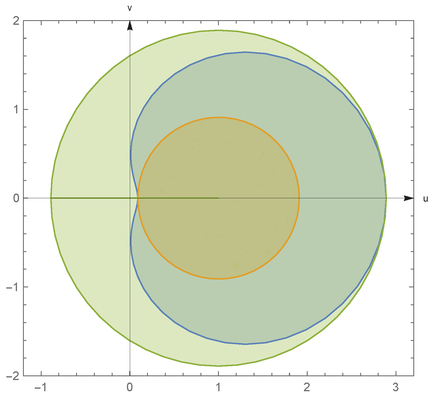
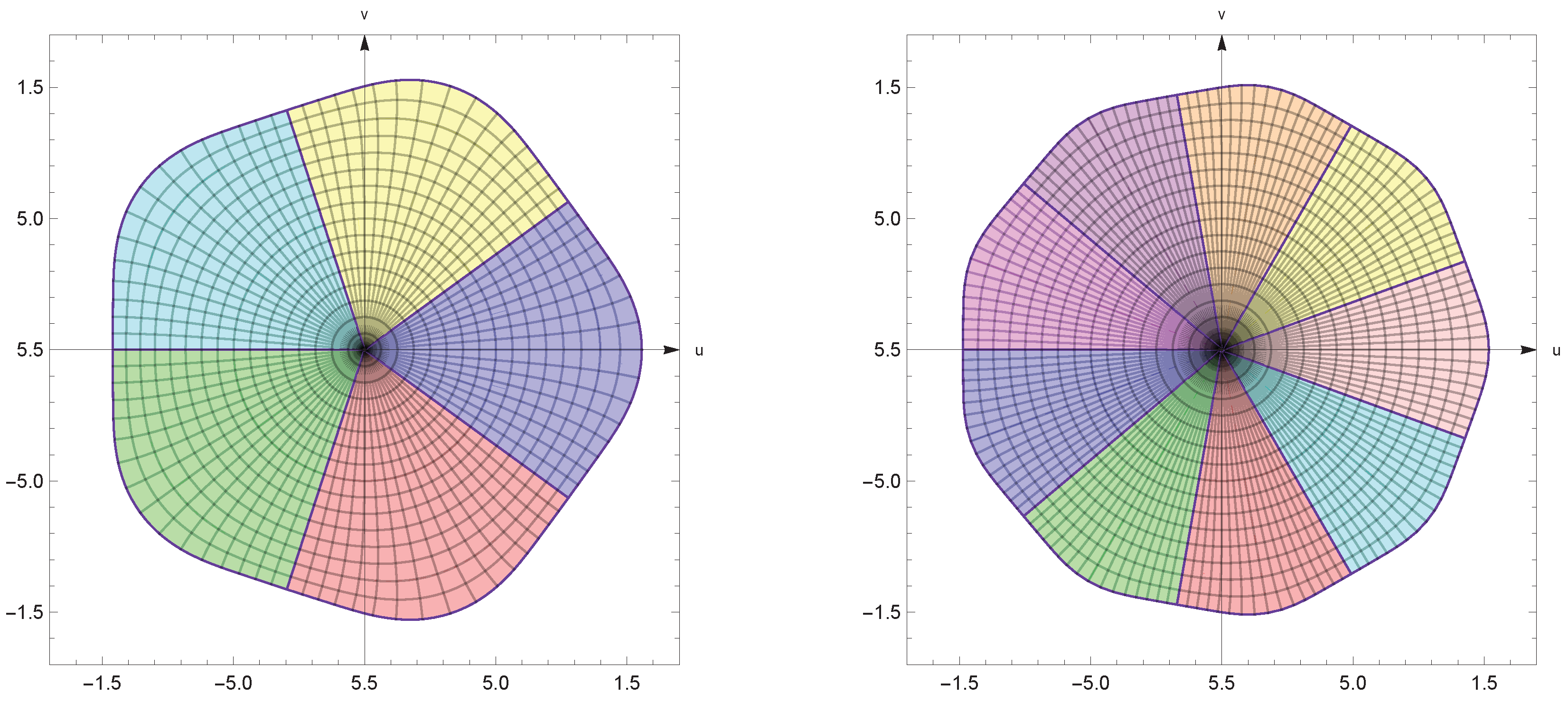
From Lemma 2 it can be seen that the smallest disk with center $(1,0)$ that contains ${\mathbb{L}}_s\left(z\right)$ and the largest disk with center at $(1,0)$ contained in ${\mathbb{L}}_s\left(z\right)$ are the following (see Figure 4)

$$\begin{array}{ccc}{\mathbb{L}}_s\left(\mathbb{D}\right)\hfill & \supset & \left\{w\in \mathbb{C}:\left|w-1\right|<1-{(1-|s\left|\right)}^2\right\},\end{array}$$

(9)

$$\begin{array}{ccc}{\mathbb{L}}_s\left(\mathbb{D}\right)\hfill & \subset & \left\{w\in \mathbb{C}:\left|w-1\right|<{(1+|s\left|\right)}^2-1\right\}.\end{array}$$

(10)

Taking into account the properties of a function ${\mathbb{L}}_s$ given in Theorem 1 and Lemma 2, we see that for $0<s\le 1/\sqrt{2}$, the function ${\mathbb{L}}_s\in {\mathcal{P}}^{\ast }$ (see also Figure 5). Additionally, those properties allow to formulate the following definition.

Definition 2.

By $\mathcal{P}\left({\mathbb{L}}_s\right)$, with $0<s\le 1/\sqrt{2}$, we denote a class of all analytic functions p such that $p\left(0\right)=1$ and $p\left(z\right)\prec {\mathbb{L}}_s\left(z\right)$ in $\mathbb{D}$, that is

$$\mathcal{P}\left({\mathbb{L}}_s\right)=\{p\left(z\right)=1+p_{1}z+p_2{z}^2+\cdots ,p\left(z\right)\prec {\mathbb{L}}_s\left(z\right),z\in \mathbb{D}\}.$$

It is clear that $\mathcal{P}\left({\mathbb{L}}_s\right)$ is a subfamily of the well-known Carathéodory class $\mathcal{P}=\mathcal{P}\left((1+z)/(1-z)\right)$ of normalized functions in $\mathbb{D}$ with positive real part.

On the basis of the relationship between subclasses of the Carathéodory class and the notion of classical starlikeness and convexity we also define the following classes.

Definition 3.

Let ${\mathcal{ST}}_L\left(s\right)$ denote the subfamily of $\mathcal{A}$ consisting of the functions f, satisfying the condition

$$\frac{z{f}^{\prime }\left(z\right)}{f\left(z\right)}\prec {\mathbb{L}}_s\left(z\right)\mathit{for}z\in \mathbb{D},0<s\le \frac{1}{\sqrt{2}}$$

(11)

and let ${\mathcal{CV}}_L\left(s\right)$ be a class of analytic functions f such that

$$1+\frac{z{f}^{″}\left(z\right)}{f^{\prime }\left(z\right)}\prec {\mathbb{L}}_s\left(z\right)\mathit{for}z\in \mathbb{D},0<s\le \frac{1}{\sqrt{2}}.$$

(12)

From Theorem 1, we obtain that for $f\in {\mathcal{ST}}_L\left(s\right)$ (and $f\in {\mathcal{CV}}_L\left(s\right)$, respectively), it holds

$$\Re \left\{\frac{z{f}^{\prime }\left(z\right)}{f\left(z\right)}\right\}>m_0\left(s\right)\mathit{for}z\in \mathbb{D},0<s\le \frac{1}{\sqrt{2}}$$

and

$$\Re \left\{1+\frac{z{f}^{″}\left(z\right)}{f^{\prime }\left(z\right)}\right\}>m_0\left(s\right)\mathit{for}z\in \mathbb{D},0<s\le \frac{1}{\sqrt{2}},$$

where $m_0\left(s\right)$ is given in Theorem 1. Geometrically, the condition Equations (11) and (12) mean that the expression $z{f}^{\prime }\left(z\right)/f\left(z\right)$ or $1+z{f}^{″}\left(z\right)/f^{\prime }\left(z\right)$ lies in a domain bounded by the limaçon $\partial \mathfrak{D}\left(s\right)$. Since a domain ${\mathbb{L}}_s\left(\mathbb{D}\right)$ is contained in a right half-plane, we deduce that ${\mathcal{ST}}_L\left(s\right)$$({\mathcal{CV}}_L\left(s\right)$, resp.) is a proper subset of a starlike functions $\mathcal{ST}$ (convex function $\mathcal{CV}$, resp.). Further properties of ${\mathbb{L}}_s\left(\mathbb{D}\right)$ yield:

$${\mathcal{ST}}_L\left(s\right)\subset \mathcal{ST}\left(\gamma \right),{\mathcal{CV}}_L\left(s\right)\subset \mathcal{CV}\left(\gamma \right)\mathit{with}0\le \gamma \le m_0\left(s\right).$$

Additionally,

$$({\mathbb{L}}_s\left(z\right)-1)/\left(2s\right)\in \left\{\begin{array}{cc}\mathcal{G}\hfill & \mathit{for}0<s\le \frac{3}{5},\hfill \\ \mathcal{N}\hfill & \mathit{for}0<s\le 1.\hfill \end{array}\right.$$

$${\mathcal{ST}}_L\left(s\right)\subset \mathcal{N},{\mathcal{CV}}_L\left(s\right)\subset \mathcal{G}.$$

For a function $g\in \mathcal{A}$, we have the equivalence: $g\in {\mathcal{ST}}_L\left(s\right)$ if and only if $z{g}^{\prime }\left(z\right)/g\left(z\right)\prec {\mathbb{L}}_s\left(z\right)$. This gives the structural formula for functions in ${\mathcal{ST}}_L\left(s\right)$. A function g is in the class ${\mathcal{ST}}_L\left(s\right)$ if and only if there exists an analytic function $p\in \mathcal{P}\left({\mathbb{L}}_s\right)$, such that

$$g\left(z\right)=zexp\left({\int }_0^z\frac{p\left(t\right)-1}{t}\mathrm{d}t\right)\mathrm{for}\mathrm{some}p\mathrm{with}p\prec {\mathbb{L}}_s.$$

This integral representation supply many examples of functions in class ${\mathcal{ST}}_L\left(s\right)$. For $n=1,2,3,\dots$, we define the functions ${\mathsf{\Psi }}_{s,n}\left(z\right)$ in ${\mathcal{ST}}_L\left(s\right)$ by the relation

$$\frac{z{\mathsf{\Psi }}_{s,n}^{\prime }\left(z\right)}{{\mathsf{\Psi }}_{s,n}\left(z\right)}={\mathbb{L}}_s\left(z^n\right),$$

namely,

$$\begin{array}{cc}\hfill {\mathsf{\Psi }}_{s,n}\left(z\right)& =zexp\left({\int }_0^z\frac{{\mathbb{L}}_s\left(t^n\right)-1}{t}\mathrm{d}t\right)=zexp\left(\frac{2s}{n}{z}^n+\frac{s^2}{2n}{z}^{2n}\right)\hfill \\ \hfill & =z+\frac{2s}{n}{z}^{n+1}+\frac{(n+4)s^2}{2n^2}{z}^{2n+1}+\cdots .\hfill \end{array}$$

(13)

These functions are extremal for several problems in the class ${\mathcal{ST}}_L\left(s\right)$ (see Figure 6).

For instance, we have

$${\mathsf{\Psi }}_s\left(z\right):={\mathsf{\Psi }}_{s,1}\left(z\right)=zexp\left(2sz+\frac{s^2}{2}{z}^2\right)=z+2s{z}^2+\frac{5}{2}{s}^2{z}^3+\cdots .$$

(14)

For a function $h\in \mathcal{A}$, we have the equivalence: $h\in {\mathcal{CV}}_L\left(s\right)$ if and only if $z{h}^{″}\left(z\right)/h^{\prime }\left(z\right)\prec {\mathbb{L}}_s\left(z\right)$. This gives the structural formula for functions in ${\mathcal{CV}}_L\left(s\right)$. A function h is in the class ${\mathcal{CV}}_L\left(s\right)$ if and only if there exists an analytic function p with $p\in \mathcal{P}\left({\mathbb{L}}_s\right)$, such that

$$h\left(z\right)={\int }_0^{z}exp\left({\int }_0^w\frac{p\left(t\right)-1}{t}\mathrm{d}t\right)\mathrm{d}w.$$

This above integral representation supply many examples of functions in class ${\mathcal{CV}}_L\left(s\right)$. Let $p\left(z\right)={\mathbb{L}}_s\left(z^n\right)\in {\mathcal{CV}}_L\left(s\right)$, then the functions (see Figure 7)

$$K_{s,n}\left(z\right)={\int }_0^{z}exp\left(\frac{2s}{n}{t}^n+\frac{s^2}{2n}{t}^{2n}\right)\mathrm{d}t=z+\frac{2s}{n(n+1)}{z}^{n+1}+\cdots ,$$

(15)

for some $n\ge 1$ are extremal functions for several problems in the class ${\mathcal{CV}}_L\left(s\right)$. For $n=1$ we have

$$K_s\left(z\right):=K_{s,1}\left(z\right)={\int }_0^{z}exp\left(2st+\frac{s^2}{2}{t}^2\right)\mathrm{d}t=z+s{z}^2+\cdots .$$

(16)

From Equation (9), a function $f\in \mathcal{A}$ is in ${\mathcal{ST}}_L\left(s\right)$ if and only if

$$\left|\frac{z{f}^{\prime }\left(z\right)}{f\left(z\right)}-1\right|<L_0\le 1-{(1-s)}^2\mathit{for}z\in \mathbb{D}.$$

(17)

Thus we have the following result.

Proposition 1.

Let $0<s\le 1/\sqrt{2}$. The classes ${\mathcal{ST}}_L\left(s\right)$ and ${\mathcal{CV}}_L\left(s\right)$ are nonempty. The following functions are the examples of their members.

• Let $a_n\in \mathbb{C}$ with $n=2,3,\dots$. Then $f\left(z\right)=z+a_n{z}^n\in {\mathcal{ST}}_L\left(s\right)$$⟺\left|a_n\right|\le \frac{1-{(1-s)}^2}{n-{(1-s)}^2}.$
• Let $a_n\in \mathbb{C}$ with $n=2,3,\dots$. Then $f\left(z\right)=z+a_n{z}^n\in {\mathcal{CV}}_L\left(s\right)$$⟺n\left|a_n\right|\le \frac{1-{(1-s)}^2}{n-{(1-s)}^2}.$
• Let $A\in \mathbb{C}$. Then $z/{(1-Az)}^2\in {\mathcal{ST}}_L\left(s\right)⟺\left|A\right|\le \frac{1-{(1-s)}^2}{1+{(1-s)}^2}.$
• Let $A\in \mathbb{C}$. Then $z/(1-Az)\in {\mathcal{CV}}_L\left(s\right)⟺\left|A\right|\le \frac{1-{(1-s)}^2}{1+{(1-s)}^2}.$
• Let $A\in \mathbb{C}$. Then $z/(1-Az)\in {\mathcal{ST}}_L\left(s\right)⟺\left|A\right|\le \frac{1+{(1-s)}^2}{2+{(1-s)}^2}.$
• Let $A\in \mathbb{C}$. Then $\frac{-ln(1-Az)}{A}\in {\mathcal{CV}}_L\left(s\right)⟺0<\left|A\right|\le \frac{1+{(1-s)}^2}{2+{(1-s)}^2}.$
• Let $A\in \mathbb{C}$. Then $zexp\left(Az\right)\in {\mathcal{ST}}_L\left(s\right)⟺\left|A\right|\le 1-{(1-s)}^2.$
• Let $A\in \mathbb{C}$. Then $\frac{exp\left(Az\right)-1}{A}\in {\mathcal{CV}}_L\left(s\right)⟺0<\left|A\right|\le 1-{(1-s)}^2.$

Proof. 

The function $f\left(z\right)=z+a_n{z}^n$ is univalent, if and only if $|a_n|\le 1/n$. Logarithmic differentiation of a non-zero univalent function $f\left(z\right)/z$ in $\mathbb{D}$ yields:

$$\frac{z{f}^{\prime }\left(z\right)}{f\left(z\right)}-1=\frac{(n-1)a_n{z}^{n-1}}{1+a_n{z}^{n-1}}\mathit{for}z\in \mathbb{D}.$$

Thus

$$\left|\frac{z{f}^{\prime }\left(z\right)}{f\left(z\right)}-1\right|=\left|\frac{(n-1)a_n{z}^{n-1}}{1+a_n{z}^{n-1}}\right|<\frac{(n-1)|a_n|}{1-|a_n|}\mathit{for}z\in \mathbb{D}.$$

From Equation (17), the function $z+a_n{z}^n$ is in ${\mathcal{ST}}_L\left(s\right)$ if and only if

$$\frac{(n-1)|a_n|}{1-|a_n|}\le 1-{(1-s)}^2.$$

Thus the case (1) is obtained. The second type obtained of the former and the fact that $f\in {\mathcal{CV}}_L\left(s\right)$ if and only if $z{f}^{\prime }\in {\mathcal{ST}}_L\left(s\right)$. The argumentation of the other cases is similar to arguments (1) and (2). □

The following corollary is the consequence of Lemma 2, and Theorems in [4].

Corollary 1.

If $f\in {\mathcal{ST}}_L\left(s\right)$ and $\left|z\right|=r<1$, then

1. 

$-{\mathsf{\Psi }}_s(-r)\le \left|f\left(z\right)\right|\le {\mathsf{\Psi }}_s\left(r\right),$

2. 

${\mathsf{\Psi }}_s^{\prime }(-r)\le \left|f^{\prime }\left(z\right)\right|\le {\mathsf{\Psi }}_s^{\prime }\left(r\right),$

3. 

$\left|\mathsf{Arg}\{f\left(z\right)/z\}\right|\le 2sr+\left(s^2{r}^2\right)/2$

Equality holds at a given point other than 0 for functions $\overline{\mu }{\mathsf{\Psi }}_s\left(\mu z\right)$ with $\left|\mu \right|=1$.

4. 

$f\left(z\right)/z\prec {\mathsf{\Psi }}_s\left(z\right)/z\left(z\in \mathbb{D}\right),$

5. 

If $f\in {\mathcal{ST}}_L\left(s\right)$, then either f is a rotation of ${\mathsf{\Psi }}_s$ given by Equation (14) or $\{w\in \mathbb{C}:\left|w\right|\le -{\mathsf{\Psi }}_s(-1)$$=exp(s^2/2-2s)\}\subset f\left(\mathbb{D}\right),$ where $-{\mathsf{\Psi }}_s(-1)={lim}_{r\to 1^{+}}-{\mathsf{\Psi }}_s(-r)$.

Corollary 2.

If $f\in {\mathcal{CV}}_L\left(s\right)$ and $\left|z\right|=r<1$, then

1. 

$-K_s(-r)\le \left|f\left(z\right)\right|\le K_s\left(r\right),$

2. 

$K_s^{\prime }(-r)\le \left|f^{\prime }\left(z\right)\right|\le K_s^{\prime }\left(r\right),$

3. 

$\left|\mathsf{Arg}\left\{f^{\prime }\left(z\right)\right\}\right|\le 2sr+\left(s^2{r}^2\right)/2,$

Equality holds at a given point other than 0 for functions $\overline{\mu }{K}_s\left(\mu z\right)$ with $\left|\mu \right|=1$.

4. 

$f^{\prime }\left(z\right)\prec K_s^{\prime }\left(z\right)\left(z\in \mathbb{D}\right),$

5. 

If $f\in {\mathcal{CV}}_L\left(s\right)$, then either f is a rotation of $K_s$ given by Equation (16) or $\{w\in \mathbb{C}:|w|\le$$-K_s(-1)\}\subset f\left(\mathbb{D}\right),$ where $-K_s(-1)={lim}_{r\to 1^{+}}-K_s(-r)$.

Theorem 2.

Let p be an analytic function in $\mathbb{D}$ with $p\left(0\right)=1$. Then for $z\in \mathbb{D}$

$$\frac{z{p}^{\prime }\left(z\right)}{p\left(z\right)}\prec \frac{z{\mathbb{L}}_s^{\prime }\left(z\right)}{{\mathbb{L}}_s\left(z\right)}⟹p\in \mathcal{P}\left({\mathbb{L}}_s\right)\mathit{for}0<s\le \frac{1}{\sqrt{2}}$$

(18)

and ${\mathbb{L}}_s$ is the best dominant.

Proof. 

If we take $\mathsf{\Phi }\left(z\right)=1/z$ and $q\equiv {\mathbb{L}}_s$, then for $0<s\le 1/\sqrt{2}$, the domain $\mathsf{\Phi }\left(\mathbb{D}\right)$ containing ${\mathbb{L}}_s\left(\mathbb{D}\right)$ and by Lemma 2

$$z{q}^{\prime }\left(z\right)\mathsf{\Phi }\left(q\left(z\right)\right)=\frac{z{\mathbb{L}}_s^{\prime }\left(z\right)}{{\mathbb{L}}_s\left(z\right)}=\frac{2sz}{1+sz}$$

is starlike. Therefore, by Lemma 1 we deduce the assertion. □

If we take $p\left(z\right)=z{f}^{\prime }\left(z\right)/f\left(z\right)$, $p\left(z\right)=f\left(z\right)/z$, $p\left(z\right)=z/f\left(z\right)$ and $p\left(z\right)=f^{\prime }\left(z\right)$ in Theorem 1 we obtain the following results.

Corollary 3.

Let $f\in \mathcal{A}$ and $0<s\le 1/\sqrt{2}$. Then

$$\begin{array}{ccc}1+\frac{z{f}^{″}\left(z\right)}{f^{\prime }\left(z\right)}-\frac{z{f}^{\prime }\left(z\right)}{f\left(z\right)}\prec \frac{2sz}{1+sz}\hfill & ⟹& f\in {\mathcal{ST}}_L\left(s\right),\\ \frac{z{f}^{\prime }\left(z\right)}{f\left(z\right)}\prec \frac{1+3sz}{1+sz}\hfill & ⟹& f\left(z\right)/z\in \mathcal{P}\left({\mathbb{L}}_s\right),\\ \frac{z{f}^{\prime }\left(z\right)}{f\left(z\right)}\prec \frac{1-sz}{1+sz}\hfill & ⟹& z/f\left(z\right)\in \mathcal{P}\left({\mathbb{L}}_s\right),\\ 1+\frac{z{f}^{″}\left(z\right)}{f^{\prime }\left(z\right)}\prec \frac{1+3sz}{1+sz}\hfill & ⟹& f^{\prime }\in \mathcal{P}\left({\mathbb{L}}_s\right).\end{array}$$

Theorem 3.

Let p be an analytic function in $\mathbb{D}$ with $p\left(0\right)=1$. Then for $z\in \mathbb{D}$

$$z{p}^{\prime }\left(z\right)\prec z{\mathbb{L}}_s^{\prime }\left(z\right)⟹p\in \mathcal{P}\left({\mathbb{L}}_s\right)\mathit{for}0<s\le \frac{1}{2}$$

(19)

and ${\mathbb{L}}_s$ is the best dominant.

Proof. 

If we take $\mathsf{\Phi }\equiv 1$ and $q\equiv {\mathbb{L}}_s$, then the domain $\mathsf{\Phi }\left(\mathbb{D}\right)$ containing ${\mathbb{L}}_s\left(\mathbb{D}\right)$ and by Lemma 2

$$z{q}^{\prime }\left(z\right)\mathsf{\Phi }\left(q\left(z\right)\right)=z{\mathbb{L}}_s^{\prime }\left(z\right)=2sz(1+sz)\mathit{for}0<s\le \frac{1}{2}$$

is starlike. Therefore, by Lemma 1 we deduce the Theorem. □

If we take $p\left(z\right)=f^{\prime }\left(z\right)$ in Theorem 3 we obtain the following result.

Corollary 4.

Let $f\in \mathcal{A}$ and $0<s\le 1/2$. Then

$$z{f}^{″}\left(z\right)\prec 2sz(1+sz)⟹f^{\prime }\in \mathcal{P}\left({\mathbb{L}}_s\right).$$

4. Conclusions

The paper presents exhaustive characteristics of the curve called limaçon of Pascal, taking into account various parameters. Families of convex and starlike functions associated with the limaçon of Pascal, for which standard functionals are located in the domains bounded by the limaçon curve. Examples and properties of extremal functions in defined families were also presented.