Goal Programming Models with Linear and Exponential Fuzzy Preference Relations

Abstract

Goal programming (GP) is a powerful method to solve multi-objective programming problems. In GP the preferential weights are incorporated in different ways into the achievement function. The problem becomes more complicated if the preferences are imprecise in nature, for example ‘Goal A is slightly or moderately or significantly important than Goal B’. Considering such type of problems, this paper proposes standard goal programming models for multi-objective decision-making, where fuzzy linguistic preference relations are incorporated to model the relative importance of the goals. In the existing literature, only methods with linear preference relations are available. As per our knowledge, nonlinearity was not considered previously in preference relations. We formulated fuzzy preference relations as exponential membership functions. The grades or achievement function is described as an exponential membership function and is used for grading levels of preference toward uncertainty. A nonlinear membership function may lead to a better representation of the achievement level than a linear one. Our proposed models can be a useful tool for different types of real life applications, where exponential nonlinearity in goal preferences exists. Finally, a numerical example is presented and analyzed through multiple cases to validate and compare the proposed models. A distance measure function is also developed and used to compare proposed models. It is found that, for the numerical example, models with exponential membership functions perform better than models with linear membership functions. The proposed models will help decision makers analyze and plan real life problems more realistically.

1. Introduction

Multi-objective mathematical programming is a powerful mathematical procedure and applicable in decision making to a wide range of real life problems [1,2,3,4,5]. A multi-objective mathematical programming model consists of multiple objective functions, constraints, and decision variables and can be stated as follows:

$$\begin{array}{cc}\hfill \mathrm{Max}(\mathrm{Min}):& \left\{f_1(x),f_2(x),\dots ,f_K(x)\right\},\hfill \end{array}$$

(1)

$$\begin{array}{cc}\hfill \mathrm{subject}\mathrm{to}& Ax\le b\hfill \end{array}$$

(2)

$$\begin{array}{cc}\hfill & x\ge 0,x\in S.\hfill \end{array}$$

(3)

where $f_k(x)$ for all $k=1,2,\dots ,K$ is a function of a decision variable x and S is the set of feasible solutions. Here, Equation (2) represents the constraints where A and b are the $m\times n$ and $n\times 1$ matrices, respectively. The ideal solution for a multiple objective programming problem would be to find a solution x, which optimizes each individual objective function of the problem, simultaneously. However, with the conflicting objectives in the model, a feasible solution that optimizes one objective may not optimize any of the other remaining objective functions. Considering this difficulty, several methodologies have been developed to handle the problem of multiple objectives.

Goal Programming (GP) is one of the widely used technique to solve multi-objective optimization problems. It was initially proposed by Charnes and Cooper [6], Charnes et al. [7] and further extended by Caballero et al. [8], Chang [9], Ignizio [10,11], Romero [12,13] and others. GP deals with the over (positive) and under (negative) achievement of the goals in such a manner that each objective is satisfied with the least deviation from its respective goal. In classical GP, the aspiration level of goals are considered as precise and deterministic. However, in real life, when the aspiration levels are not precise in nature, the concept of fuzzy uncertainty can be applied. The fuzzy set theory was first introduced by Zadeh [14]. Bellman and Zadeh [15] further developed a decision theory in a fuzzy environment. Moreover, the uncertainty involved due to vagueness and ambiguity is being dealt within the fuzzy domain.

When fuzzy set theory is introduced in goal programming, it became fuzzy goal programming. Using fuzzy goal programming, the degree of satisfaction of each objective function is maximized which helps the decision maker to decide the best efficient solution. Many researchers proposed and applied fuzzy goal programming models, for example Aköz and Petrovic [16], Anukokila et al. [17], Chen and Tsai [18], Cheng [19], Dalman and Bayram [20], Díaz-Madronero et al. [21], Hocine et al. [22], Jadidi et al. [23], Jamalnia and Soukhakian [24], Jiménez et al. [25], Pramanik and Roy [26], and Jana et al. [27]. It is not always possible that the goals priority is symmetric in nature. The decisions become more complicated, when the problem has imprecise preferences for the priorities of the goals and their aspiration levels. In 2007, Aköz and Petrovic [16] proposed a fuzzy goal programming model with an imprecise linear goal hierarchy. They used a linear membership function for three type of linguistic fuzzy preference relations, i.e., Goal A is “slightly” or “moderately” or “significantly more important” than Goal B. The preference relations are of asymmetric nature in importance of goals. After Aköz and Petrovic [16], the fuzzy preference relation was applied and extended by many authors, e.g., Cheng [19], Petrovic and Aköz [28], Torabi and Moghaddam [29], Khalili-Damghani and Sadi-Nezhad [30], Díaz-Madronero et al. [31], Sheikhalishahi and Torabi [32], Bilbao-Terol et al. [33,34], Arenas-Parra et al. [35] Hasan et al. [36], and Hashmi et al. [37]. Khalili-Damghani and Sadi-Nezhad [30], Khalili-Damghani et al. [38] extended the work of Aköz and Petrovic [16]; they extended the linear membership function for three linguistic preference terms to ten statements. Further, it was applied by Khalili-Damghani et al. [39] in a supply chain network model.

Fuzzy membership functions are used to define the aspiration levels of a decision maker. It describes the nature of fuzzy values, data, preferences, etc. Since the behavior of different fuzzy quantities may vary, the corresponding fuzzy membership functions are of different types, for example, linear, exponential, logistic, hyperbolic, parabolic, S-curve, and tangent. Decision makers may choose the membership function which fits best to their problem. Many authors applied and analyzed their problem models using linear and nonlinear membership functions. A linear membership function is perhaps the simplest and most common one, as it bounds the upper and lower acceptance levels. In nonlinear membership functions, the marginal rate of increase or decrease of membership values as a function of model parameters is not constant. Hence, it reflects the practical situations better than the linear case. Some of the authors who applied nonlinear membership functions are Anoop Kumar Dhingra and Moskowitz [40], Peidro and Vasant [41], Zangiabadi and Maleki [42], Gupta et al. [43], Ehsani et al. [44], Dhodiya and Tailor [45], and Singh and Yadav [46].

In this paper, Standard goal programming models with fuzzy goal hierarchies are proposed. The problem considered is a multi-objective optimization model having linguistic preferences among the objectives, for example “significantly more important”, “moderately more important”, and “slightly more important”, and can be expressed as follows:

$$\begin{array}{cc}\hfill \mathrm{FuzzyHierMax}:& \left\{f_1(x),f_2(x),\dots ,f_K(x)\right\},\hfill \end{array}$$

(4)

$$\begin{array}{cc}\hfill \mathrm{subject}\mathrm{to}& Ax\le b\hfill \end{array}$$

(5)

$$\begin{array}{cc}\hfill & x\ge 0,x\in S.\hfill \end{array}$$

(6)

Here, “FuzzyHierMax” denotes the fuzzy hierarchical maximization for achieving the satisfactory solution considering the preferences among the objectives. The proposed GP models are the extensions to existing models of Aköz and Petrovic [16], Arenas-Parra et al. [35]. The preferences among the goals $\left\{f_1(x),f_2(x),\dots ,f_K(x)\right\}$ are assumed as fuzzy, having linear and exponential membership functions. The results for different models due to linear and exponential membership functions are further presented and compared. In real life problems, preferences among goals may be of exponential nature. To deal with nonlinearity, we formulated the exponential membership function for ten types of linguistic preference relations, which is the extension to the linear membership function which was earlier proposed by Aköz and Petrovic [16], Khalili-Damghani and Sadi-Nezhad [30], and Khalili-Damghani et al. [38]. Four goal programming models are formulated along with the solution approach. As per our knowledge, in existing literature, there is no GP model with proposed exponential membership function for relative preferences between the goals. In the proposed GP model, we take account of maximization of the minimum and the sum of achievements of goals using approaches from Arenas-Parra et al. [35], Torabi and Hassini [47]. Hence, this work address the research gap, and helps the decision maker to plan more realistically by introducing exponential type preference relations. To analyze the performance of proposed models, we developed a distance measure function. It helps to determine the degree of closeness of the result to the ideal solution.

In this paper, Section 2 presents the proposed goal programming formulations. In Section 3, the solution approach along with flow diagram is presented. In Section 4, an experimental study is performed along with efficiency measure analysis to validate the proposed models. Finally, Section 5 presents the conclusion.

2. Goal Programming Formulation

This section presents the goal programming formulation of proposed models with fuzzy hierarchy among the goals. Before moving to the GP, we first go through the formulation of normalized function and membership functions of preference relations for linear as well as exponential case. To avoid biasedness towards goals with high and low aspiration levels, Arenas-Parra et al. [35] used a normalized function corresponding to each objective. Let us assume that $\underline{f_k}$ and $f_k^{\ast }$, $k=1,\dots ,K$, are the anti-ideal and aspiration values of objective $f_k$, respectively. An anti-ideal value is the worst value of an objective function, whereas an aspiration value is the desired value of an objective function by the decision maker. Now, the normalized function ($n_k$) for objective function $f_k$ can be modeled as:

$$n_k=1-\left|{\displaystyle \frac{(d_k^{-}+d_k^{+})}{(f_k^{\ast }-\underline{f_k})}}\right|.$$

(7)

In Equation (7), $d_k^{-}$ and $d_k^{+}$ represent the negative and positive deviation of the objectives $f_k$ from $f_k^{\ast }$. The deviations must satisfy the condition, $d_k^{-}·d_k^{+}=0,\forall k\in 1,\dots ,K$. The normalized value satisfies the following property

$$0\le n_k\le 1.$$

(8)

If the kth objective is more important than the lth objective, then the kth normalized deviation is greater than or equal to that of the lth objective. Hence, we have

$$n_l\le n_k.$$

(9)

However, the normalization constraint may lead to an infeasible solution, as it is a strict relation. To avoid this infeasibility, Arenas-Parra et al. [35] applied the approach of Aköz and Petrovic [16], which expresses preferences among goals in terms of fuzzy relations.

2.1. Representation of Fuzzy Preference Relations as Membership Functions

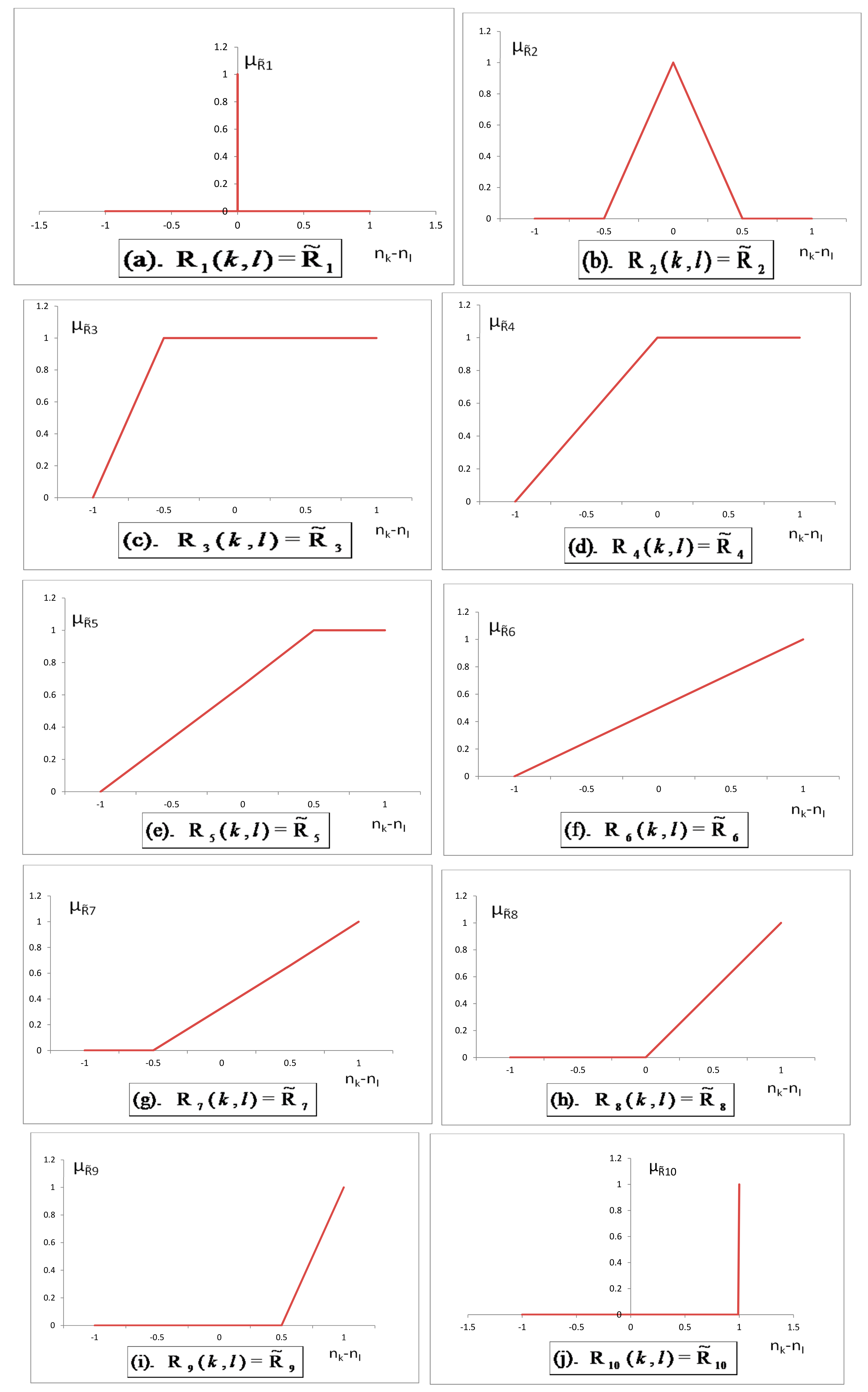
In 2007, Aköz and Petrovic [16] proposed linear membership functions for three type of fuzzy imprecise preferences namely “slightly more important than”, “moderately more important than”, and “significantly more important than”, to describe the imprecise relative importance relations among the goals. Later in 2013, Khalili-Damghani and Sadi-Nezhad [30] and Khalili-Damghani et al. [38] extended these linear membership functions to ten different linear membership functions. They introduced ten type of linguistic imprecise preference statements alongwith their formulations. The hierarchy structure of ten different linguistic preference relations for linear as well as exponential type is presented in Figure 1. A brief presentation of the figures and linear formulations of membership functions is given in Figure 2 and Equations (10a)–(10j), respectively.

In the present work, the formulation of a type of nonlinear membership function, i.e., exponential membership function, for fuzzy goal hierarchies is presented. More formally, we develop a procedure using a wide range of linguistic terms, different fuzzy priority relations for the decision makers preferences on the normalized values of the goals, and their associated membership functions. The details of the linguistic terms and their associated fuzzy nonlinear membership functions (${\mu }_{{\tilde{R}}_q},q=1,\dots ,10$) are shown in

Table 1. Linguistic relative preferences of objective k over l.

Linguistic Term	Fuzzy Relation	Membership Values	Transform Function
	${\tilde{\mathit{R}}}_{\mathit{q}},\mathit{q}=\mathbf{1},\mathbf{\dots },\mathbf{10}$	${\mathit{\mu }}_{{\tilde{\mathit{R}}}_{\mathit{q}}}$
Exactly equal	${\tilde{R}}_1$	${\mu }_{{\tilde{R}}_1}$
Partially equal	${\tilde{R}}_2$	${\mu }_{{\tilde{R}}_2}$
Partially more important than	${\tilde{R}}_3$	${\mu }_{{\tilde{R}}_3}$
Slightly more important than	${\tilde{R}}_4$	${\mu }_{{\tilde{R}}_4}$
Moderately more important than	${\tilde{R}}_5$	${\mu }_{{\tilde{R}}_5}$	${\mu }_k(X)-{\mu }_l(X)$
Significantly more important than	${\tilde{R}}_6$	${\mu }_{{\tilde{R}}_6}$	$\forall k,l\in 1,\dots ,K$
Completely more important than	${\tilde{R}}_7$	${\mu }_{{\tilde{R}}_7}$
Fully more important than	${\tilde{R}}_8$	${\mu }_{{\tilde{R}}_8}$
Extremely more important than	${\tilde{R}}_9$	${\mu }_{{\tilde{R}}_9}$
Incomparable	${\tilde{R}}_{10}$	${\mu }_{{\tilde{R}}_{10}}$

. The table has four columns with type of linguistic term, notation for the fuzzy relation, membership function, and finally the transform function to formulate the preference membership functions.

$$\begin{array}{cc}\hfill {\mu }_{{\tilde{R}}_1(k,l)}& =\left\{\begin{array}{cc}0,\hfill & \mathrm{if}-1\le n_k-n_l<0;\hfill \\ 1,\hfill & \mathrm{if}{n}_k-n_l=0;\hfill \\ 0,\hfill & \mathrm{if}0<n_k-n_l\le 1.\hfill \end{array}\right.\hfill \end{array}$$

(10a)

$$\begin{array}{cc}\hfill {\mu }_{{\tilde{R}}_2(k,l)}& =\left\{\begin{array}{cc}0,\hfill & \mathrm{if}-1\le n_k-n_l\le -0.5;\hfill \\ 2(n_k-n_l+0.5),\hfill & \mathrm{if}-0.5\le n_k-n_l\le 0;\hfill \\ -2(n_k-n_l+0.5),\hfill & \mathrm{if}0\le n_k-n_l\le 0.5;\hfill \\ 0,\hfill & \mathrm{if}0.5\le n_k-n_l\le 1.\hfill \end{array}\right.\hfill \end{array}$$

(10b)

$$\begin{array}{cc}\hfill {\mu }_{{\tilde{R}}_3(k,l)}& =\left\{\begin{array}{cc}2(n_k-n_l+1),\hfill & \mathrm{if}-1\le n_k-n_l\le -0.5;\hfill \\ 1,\hfill & \mathrm{if}-0.5\le n_k-n_l\le 1.\hfill \end{array}\right.\hfill \end{array}$$

(10c)

$$\begin{array}{cc}\hfill {\mu }_{{\tilde{R}}_4(k,l)}& =\left\{\begin{array}{cc}(n_k-n_l+1),\hfill & \mathrm{if}-1\le n_k-n_l\le 0;\hfill \\ 1,\hfill & \mathrm{if}0\le n_k-n_l\le 1.\hfill \end{array}\right.\hfill \end{array}$$

(10d)

$$\begin{array}{cc}\hfill {\mu }_{{\tilde{R}}_5(k,l)}& =\left\{\begin{array}{cc}\frac{2}{3}(n_k-n_l+1),\hfill & \mathrm{if}-1\le n_k-n_l\le 0.5;\hfill \\ 1,\hfill & \mathrm{if}0.5\le n_k-n_l\le 1.\hfill \end{array}\right.\hfill \end{array}$$

(10e)

$$\begin{array}{cc}\hfill {\mu }_{{\tilde{R}}_6(k,l)}& =\left\{\begin{array}{cc}(\frac{n_k-n_l+1}{2}),\hfill & \mathrm{if}-1\le n_k-n_l\le 1.\hfill \end{array}\right.\hfill \end{array}$$

(10f)

$$\begin{array}{cc}\hfill {\mu }_{{\tilde{R}}_7(k,l)}& =\left\{\begin{array}{cc}1,\hfill & \mathrm{if}-1\le n_k-n_l\le -0.5;\hfill \\ \frac{2}{3}(n_k-n_l+0.5),\hfill & \mathrm{if}-0.5\le n_k-n_l\le 1.\hfill \end{array}\right.\hfill \end{array}$$

(10g)

$$\begin{array}{cc}\hfill {\mu }_{{\tilde{R}}_8(k,l)}& =\left\{\begin{array}{cc}0,\hfill & \mathrm{if}-1\le n_k-n_l\le 0;\hfill \\ (n_k-n_l),\hfill & \mathrm{if}0\le n_k-n_l\le 1.\hfill \end{array}\right.\hfill \end{array}$$

(10h)

$$\begin{array}{cc}\hfill {\mu }_{{\tilde{R}}_9(k,l)}& =\left\{\begin{array}{cc}0,\hfill & \mathrm{if}-1\le n_k-n_l\le 0.5;\hfill \\ 2(n_k-n_l-0.5),\hfill & \mathrm{if}0.5\le n_k-n_l\le 1.\hfill \end{array}\right.\hfill \end{array}$$

(10i)

$$\begin{array}{cc}\hfill {\mu }_{{\tilde{R}}_{10}(k,l)}& =\left\{\begin{array}{cc}0,\hfill & \mathrm{if}-1\le n_k-n_l<1;\hfill \\ 1,\hfill & \mathrm{if}{n}_k-n_l=1.\hfill \end{array}\right.\hfill \end{array}$$

(10j)

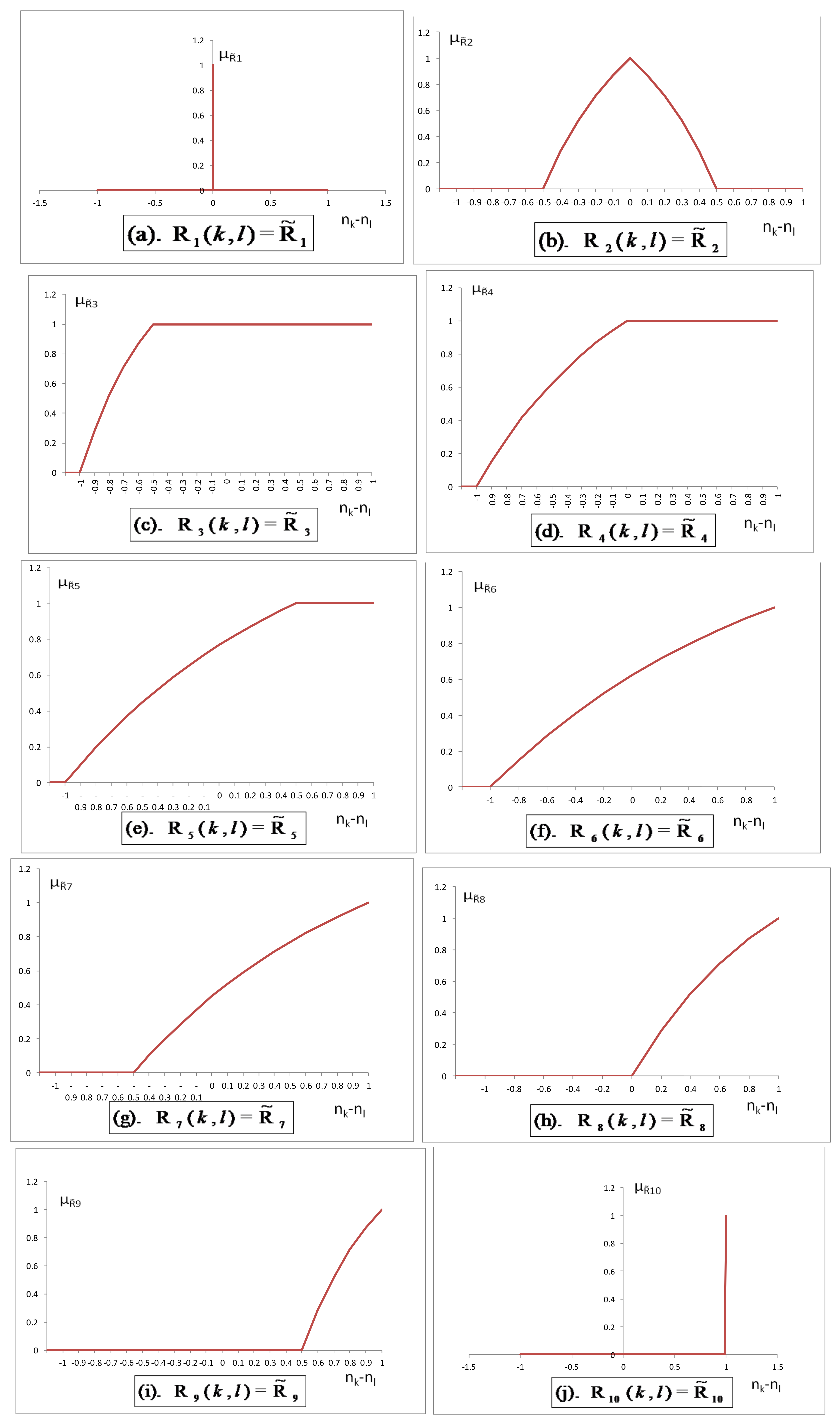
The need for introducing the grade or achievement function as a nonlinear membership function and used for grading levels of preference towards uncertainty is that it may lead to a better representation of the achievement level than a linear one. It is also good enough to represent practical situations because sometimes the marginal rate of increase or decrease of membership values is not constant always, as in the case of linear membership functions. Furthermore, the nature of the behavior of the nonlinear membership function allows itself to change its achievement values according to the parameter values, which also allow the decision maker to execute his/her strategy in a very convenient manner with flexibility. Keeping all these facts in mind, we use the exponential membership function for the achievement of the fuzzy imprecise preferences amongst the goal relations. The proposed exponential fuzzy relation membership functions are shown in Figure 3. The exponential membership function of the fuzzy relations between the goals can be formulated as given in Equations (11a)–(11j).

$$\begin{array}{cc}\hfill {\mu }_{{\tilde{R}}_1(k,l)}& =\left\{\begin{array}{cc}0,\hfill & \mathrm{if}-1\le n_k-n_l<0;\hfill \\ 1,\hfill & \mathrm{if}{n}_k-n_l=0;\hfill \\ 0,\hfill & \mathrm{if}0<n_k-n_l\le 1.\hfill \end{array}\right.\hfill \end{array}$$

(11a)

$$\begin{array}{cc}\hfill {\mu }_{{\tilde{R}}_2(k,l)}& =\left\{\begin{array}{cc}0,\hfill & \mathrm{if}-1\le n_k-n_l\le -0.5;\hfill \\ 1-{\displaystyle \frac{e^{-s·2(n_k-n_l+0.5)}-e^{-s}}{1-e^{-s}}},\hfill & \mathrm{if}-0.5\le n_k-n_l\le 0;\hfill \\ 1-{\displaystyle \frac{e^{-s·(-2(n_k-n_l+0.5))}-e^{-s}}{1-e^{-s}}},\hfill & \mathrm{if}0\le n_k-n_l\le 0.5;\hfill \\ 0,\hfill & \mathrm{if}0.5\le n_k-n_l\le 1.\hfill \end{array}\right.\hfill \end{array}$$

(11b)

$$\begin{array}{cc}\hfill {\mu }_{{\tilde{R}}_3(k,l)}& =\left\{\begin{array}{cc}1-{\displaystyle \frac{e^{-s·2(n_k-n_l+1)}-e^{-s}}{1-e^{-s}}},\hfill & \mathrm{if}-1\le n_k-n_l\le -0.5;\hfill \\ 1,\hfill & \mathrm{if}-0.5\le n_k-n_l\le 1.\hfill \end{array}\right.\hfill \end{array}$$

(11c)

$$\begin{array}{cc}\hfill {\mu }_{{\tilde{R}}_4(k,l)}& =\left\{\begin{array}{cc}1-{\displaystyle \frac{e^{-s·(n_k-n_l+1)}-e^{-s}}{1-e^{-s}}},\hfill & \mathrm{if}-1\le n_k-n_l\le 0;\hfill \\ 1,\hfill & \mathrm{if}0\le n_k-n_l\le 1.\hfill \end{array}\right.\hfill \end{array}$$

(11d)

$$\begin{array}{cc}\hfill {\mu }_{{\tilde{R}}_5(k,l)}& =\left\{\begin{array}{cc}1-{\displaystyle \frac{e^{-s·(\frac{2}{3}(n_k-n_l+1))}-e^{-s}}{1-e^{-s}}},\hfill & \mathrm{if}-1\le n_k-n_l\le 0.5;\hfill \\ 1,\hfill & \mathrm{if}0.5\le n_k-n_l\le 1.\hfill \end{array}\right.\hfill \end{array}$$

(11e)

$$\begin{array}{cc}\hfill {\mu }_{{\tilde{R}}_6(k,l)}& =\left\{\begin{array}{cc}1-{\displaystyle \frac{e^{-s·(\frac{n_k-n_l+1}{2})}-e^{-s}}{1-e^{-s}}},\hfill & \mathrm{if}-1\le n_k-n_l\le 1;.\hfill \end{array}\right.\hfill \end{array}$$

(11f)

$$\begin{array}{cc}\hfill {\mu }_{{\tilde{R}}_7(k,l)}& =\left\{\begin{array}{cc}1,\hfill & \mathrm{if}-1\le n_k-n_l\le -0.5;\hfill \\ 1-{\displaystyle \frac{e^{-s·(\frac{2}{3}(n_k-n_l+0.5))}-e^{-s}}{1-e^{-s}}},\hfill & \mathrm{if}-0.5\le n_k-n_l\le 1.\hfill \end{array}\right.\hfill \end{array}$$

(11g)

$$\begin{array}{cc}\hfill {\mu }_{{\tilde{R}}_8(k,l)}& =\left\{\begin{array}{cc}0,\hfill & \mathrm{if}-1\le n_k-n_l\le 0;\hfill \\ 1-{\displaystyle \frac{e^{-s·(n_k-n_l)}-e^{-s}}{1-e^{-s}}},\hfill & \mathrm{if}0\le n_k-n_l\le 1.\hfill \end{array}\right.\hfill \end{array}$$

(11h)

$$\begin{array}{cc}\hfill {\mu }_{{\tilde{R}}_9(k,l)}& =\left\{\begin{array}{cc}0,\hfill & \mathrm{if}-1\le n_k-n_l\le 0.5;\hfill \\ 1-{\displaystyle \frac{e^{-s·2(n_k-n_l-0.5)}-e^{-s}}{1-e^{-s}}},\hfill & \mathrm{if}0.5\le n_k-n_l\le 1.\hfill \end{array}\right.\hfill \end{array}$$

(11i)

$$\begin{array}{cc}\hfill {\mu }_{{\tilde{R}}_{10}(k,l)}& =\left\{\begin{array}{cc}0,\hfill & \mathrm{if}-1\le n_k-n_l<1;\hfill \\ 1,\hfill & \mathrm{if}{n}_k-n_l=1.\hfill \end{array}\right.\hfill \end{array}$$

(11j)

In an exponential membership function, s is the measurement of the degree of fuzziness. It can be determined by the decision maker. The parameter s is the preference of the decision maker in a fuzzy environment and can be set flexibly in different conditions. Practically, s can be selected according to the level of impreciseness of the problem. A high imprecision in decision making is reflected by a high value of s. Therefore, if the decision environment is associated with a high level of uncertainty, the decision maker should assign a higher value to s. It becomes counter-wise for the cases in which the uncertainty for decision environment is low.

2.2. Proposed Approach

Now, we explain and formulate four standard goal programming models with fuzzy preference relations (SGP-PR). Model 1 is from Arenas-Parra et al. [35] and Models 2–4 are extended goal programming models with imprecise linear and exponential goal hierarchies.

Model 1:

This model is derived from Arenas-Parra et al. [35] and considers a linear membership function for fuzzy preference relations.

Model 2:

This model is an extension of Model 1 with an integration of the proposed formulated exponential membership functions for linguistic preferences among the objectives. This model uses nonlinearities in preferences among the objectives.

Model 3:

It is another extension of Model 1, with a new objective function considering a linear membership function for linguistic preferences between the objectives.

Model 4:

It is an extension of Model 2, incorporating a new objective function and an exponential membership function for linguistic preferences.

The following are the formulations of standard goal programming models with fuzzy hierarchies:

Model 1: This model was initially proposed by Arenas-Parra et al. [35] and later utilized by Bilbao-Terol et al. [33]. Bilbao-Terol et al. [33] applied the extended model in forest planning. Here, Model 1 is the same model proposed by Arenas-Parra et al. [35] with a linear membership function for linguistic preferences among the objectives as explained. The objective functions are defined as:

$$\begin{array}{cc}\hfill \mathrm{Objective}-1:\mathrm{Maximize}& \sum _{k=1}^K{n}_k,\hfill \end{array}$$

(12a)

$$\begin{array}{cc}\hfill \mathrm{Objective}-2:\mathrm{Maximize}& \sum _{k=1}^K\sum _{l=1}^K{b}_{kl}{\mu }_{\tilde{R}(k,l)}.\hfill \end{array}$$

(12b)

Here, $b_{kl}$, for $k,l=1,2,\dots ,K$ with $k\ne l$; are binary parameters, taking the value 1 if there exists an importance relation between the goal $f_k$ and $f_l$, and 0 otherwise. A convex combination of the two objectives by applying the respective weights $\alpha$ and $(1-\alpha )$ to obtain a compromise solution between the two objectives leads to the following formulation:

$$\begin{array}{cc}\hfill & \mathrm{Maximize}Z=\alpha \left(\sum _{k=1}^K{n}_k\right)+(1-\alpha )\left(\sum _{k=1}^K\sum _{l=1}^K{b}_{kl}{\mu }_{\tilde{R}(k,l)}\right),\hfill \end{array}$$

(13a)

$$\begin{array}{cc}\hfill & \mathrm{subject}\mathrm{to}{n}_k=1-\left|{\displaystyle \frac{(d_k^{-}+d_k^{+})}{(f_k^{\ast }-\underline{f_k})}}\right|,\hfill \end{array}$$

(13b)

$$\begin{array}{cc}\hfill & f_k+d_k^{-}-d_k^{+}=f_k^{\ast },\hfill \end{array}$$

(13c)

$$\begin{array}{cc}\hfill & (n_k-n_l+1)\ge {\mu }_{{\tilde{R}}_4(k,l)},\forall b_{kl}=1\mathrm{and}\tilde{R}(k,l)={\tilde{R}}_4,\hfill \end{array}$$

(13d)

$$\begin{array}{cc}\hfill & \frac{(n_k-n_l+1)}{2}\ge {\mu }_{{\tilde{R}}_6(k,l)},\forall b_{kl}=1\mathrm{and}\tilde{R}(k,l)=\widetilde{R_6},\hfill \end{array}$$

(13e)

$$\begin{array}{cc}\hfill & (n_k-n_l)\ge {\mu }_{{\tilde{R}}_8(k,l)},\forall b_{kl}=1\mathrm{and}\tilde{R}(k,l)=\widetilde{R_8},\hfill \end{array}$$

(13f)

$$\begin{array}{cc}\hfill & {\mu }_{\tilde{R}(k,l)}\le 1,\forall b_{kl}=1,\hfill \end{array}$$

(13g)

$$\begin{array}{cc}\hfill & Ax\le b,\hfill \end{array}$$

(13h)

$$\begin{array}{cc}\hfill & x\ge 0,n_k\ge 0,\forall k=1,\dots ,K,\hfill \end{array}$$

(13i)

$$\begin{array}{cc}\hfill & n_k\le 1,\forall k=1,\dots ,K,\hfill \end{array}$$

(13j)

$$\begin{array}{cc}\hfill & d_k^{-}·d_k^{+}=0,\forall k=1,\dots ,K,\hfill \end{array}$$

(13k)

$$\begin{array}{cc}\hfill & {\mu }_{\tilde{R}(k,l)}\ge 0,\forall b_{kl}=1.\hfill \end{array}$$

(13l)

Model 2: This model is the extension of Model 1. It utilizes an exponential membership function for the fuzzy hierarchies between the goals. The formulation is presented below:

$$\begin{array}{cc}\hfill & \mathrm{Maximize}Z=\alpha \left(\sum _{k=1}^K{n}_k\right)+(1-\alpha )\left(\sum _{k=1}^K\sum _{l=1}^K{b}_{kl}{\mu }_{\tilde{R}(k,l)}\right),\hfill \end{array}$$

(14a)

$$\begin{array}{cc}\hfill & \mathrm{subject}\mathrm{to}{n}_k=1-\left|{\displaystyle \frac{(d_k^{-}+d_k^{+})}{(f_k^{\ast }-\underline{f_k})}}\right|,\hfill \end{array}$$

(14b)

$$\begin{array}{cc}\hfill & f_k+d_k^{-}-d_k^{+}=f_k^{\ast },\hfill \end{array}$$

(14c)

$$\begin{array}{cc}\hfill & 1-{\displaystyle \frac{e^{-s·(n_k-n_l+1)}-e^{-s}}{1-e^{-s}}}\ge {\mu }_{{\tilde{R}}_4(k,l)},\forall b_{kl}=1\mathrm{and}\tilde{R}(k,l)={\tilde{R}}_4,\hfill \end{array}$$

(14d)

$$\begin{array}{cc}\hfill & 1-{\displaystyle \frac{e^{-s·(\frac{n_k-n_l+1}{2})}-e^{-s}}{1-e^{-s}}}\ge {\mu }_{{\tilde{R}}_6(k,l)},\forall b_{kl}=1\mathrm{and}\tilde{R}(k,l)=\widetilde{R_6},\hfill \end{array}$$

(14e)

$$\begin{array}{cc}\hfill & 1-{\displaystyle \frac{e^{-s·(n_k-n_l)}-e^{-s}}{1-e^{-s}}}\ge {\mu }_{{\tilde{R}}_8(k,l)},\forall b_{kl}=1\mathrm{and}\tilde{R}(k,l)=\widetilde{R_8},\hfill \end{array}$$

(14f)

$$\begin{array}{cc}\hfill & {\mu }_{\tilde{R}(k,l)}\le 1,\forall b_{kl}=1\hfill \end{array}$$

(14g)

$$\begin{array}{cc}\hfill & Ax\le b,\hfill \end{array}$$

(14h)

$$\begin{array}{cc}\hfill & x\ge 0,n_k\ge 0,\forall k=1,\dots ,K,\hfill \end{array}$$

(14i)

$$\begin{array}{cc}\hfill & n_k\le 1,\forall k=1,\dots ,K,\hfill \end{array}$$

(14j)

$$\begin{array}{cc}\hfill & d_k^{-}·d_k^{+}=0,\forall k=1,\dots ,K,\hfill \end{array}$$

(14k)

$$\begin{array}{cc}\hfill & {\mu }_{\tilde{R}(k,l)}\ge 0,\forall b_{kl}=1.\hfill \end{array}$$

(14l)

Model 3: It is derived from a hybridization of the Torabi and Hassini [47] approach with the goal programming model of Arenas-Parra et al. [35]. Objective 1 in Model 1 only maximizes the sum of satisfaction levels of normalized values; it does not considers a minimum satisfaction of all the objectives. By integrating the Torabi and Hassini [47] approach, we get more flexibility as it considers both the minimum satisfaction and the sum of satisfaction of all the objectives.

$$\begin{array}{cc}\hfill & \mathrm{Maximize}Z={\gamma }_1(\lambda )+{\gamma }_2\left(\sum _{k=1}^K{n}_k\right)+{\gamma }_3\left(\sum _{k=1}^K\sum _{l=1}^K{b}_{kl}{\mu }_{\tilde{R}(k,l)}\right),\hfill \end{array}$$

(15a)

$$\begin{array}{cc}\hfill & \mathrm{subject}\mathrm{to}{n}_k=1-\left|{\displaystyle \frac{(d_k^{-}+d_k^{+})}{(f_k^{\ast }-\underline{f_k})}}\right|,\hfill \end{array}$$

(15b)

$$\begin{array}{cc}\hfill & \lambda \le n_k,\hfill \end{array}$$

(15c)

$$\begin{array}{cc}\hfill & f_k+d_k^{-}-d_k^{+}=f_k^{\ast },\hfill \end{array}$$

(15d)

$$\begin{array}{cc}\hfill & (n_k-n_l+1)\ge {\mu }_{{\tilde{R}}_4(k,l)},\forall b_{kl}=1\mathrm{and}\tilde{R}(k,l)={\tilde{R}}_4,\hfill \end{array}$$

(15e)

$$\begin{array}{cc}\hfill & \frac{(n_k-n_l+1)}{2}\ge {\mu }_{{\tilde{R}}_6(k,l)},\forall b_{kl}=1\mathrm{and}\tilde{R}(k,l)=\widetilde{R_6},\hfill \end{array}$$

(15f)

$$\begin{array}{cc}\hfill & (n_k-n_l)\ge {\mu }_{{\tilde{R}}_8(k,l)},\forall b_{kl}=1\mathrm{and}\tilde{R}(k,l)=\widetilde{R_8},\hfill \end{array}$$

(15g)

$$\begin{array}{cc}\hfill & {\mu }_{\tilde{R}(k,l)}\le 1,\forall b_{kl}=1,\hfill \end{array}$$

(15h)

$$\begin{array}{cc}\hfill & Ax\le b,\hfill \end{array}$$

(15i)

$$\begin{array}{cc}\hfill & x\ge 0,n_k\ge 0,\forall k=1,\dots ,K,\hfill \end{array}$$

(15j)

$$\begin{array}{cc}\hfill & n_k\le 1,\forall k=1,\dots ,K,\hfill \end{array}$$

(15k)

$$\begin{array}{cc}\hfill & d_k^{-}·d_k^{+}=0,\forall k=1,\dots ,K,\hfill \end{array}$$

(15l)

$$\begin{array}{cc}\hfill & {\mu }_{\tilde{R}(k,l)}\ge 0,\forall b_{kl}=1.\hfill \end{array}$$

(15m)

Model 4: This model is similar to Model 3, the only difference being in the linguistic preferences, which are represented here by an exponential membership function. Hence, Model 4 is formulated as follows:

$$\begin{array}{cc}\hfill & \mathrm{Maximize}Z={\gamma }_1(\lambda )+{\gamma }_2\left(\sum _{k=1}^K{n}_k\right)+{\gamma }_3\left(\sum _{k=1}^K\sum _{l=1}^K{b}_{kl}{\mu }_{\tilde{R}(k,l)}\right),\hfill \end{array}$$

(16a)

$$\begin{array}{cc}\hfill & \mathrm{subject}\mathrm{to}{n}_k=1-\left|{\displaystyle \frac{(d_k^{-}+d_k^{+})}{(f_k^{\ast }-\underline{f_k})}}\right|,\hfill \end{array}$$

(16b)

$$\begin{array}{cc}\hfill & \lambda \le n_k,\hfill \end{array}$$

(16c)

$$\begin{array}{cc}\hfill & f_k+d_k^{-}-d_k^{+}=f_k^{\ast },\hfill \end{array}$$

(16d)

$$\begin{array}{cc}\hfill & 1-{\displaystyle \frac{e^{-s·(n_k-n_l+1)}-e^{-s}}{1-e^{-s}}}\ge {\mu }_{{\tilde{R}}_4(k,l)},\forall b_{kl}=1\mathrm{and}\tilde{R}(k,l)={\tilde{R}}_4,\hfill \end{array}$$

(16e)

$$\begin{array}{cc}\hfill & 1-{\displaystyle \frac{e^{-s·(\frac{n_k-n_l+1}{2})}-e^{-s}}{1-e^{-s}}}\ge {\mu }_{{\tilde{R}}_6(k,l)},\forall b_{kl}=1\mathrm{and}\tilde{R}(k,l)=\widetilde{R_6},\hfill \end{array}$$

(16f)

$$\begin{array}{cc}\hfill & 1-{\displaystyle \frac{e^{-s·(n_k-n_l)}-e^{-s}}{1-e^{-s}}}\ge {\mu }_{{\tilde{R}}_8(k,l)},\forall b_{kl}=1\mathrm{and}\tilde{R}(k,l)=\widetilde{R_8},\hfill \end{array}$$

(16g)

$$\begin{array}{cc}\hfill & {\mu }_{\tilde{R}(k,l)}\le 1,\forall b_{kl}=1,\hfill \end{array}$$

(16h)

$$\begin{array}{cc}\hfill & Ax\le b,\hfill \end{array}$$

(16i)

$$\begin{array}{cc}\hfill & x\ge 0,n_k\ge 0,\forall k=1,\dots ,K,\hfill \end{array}$$

(16j)

$$\begin{array}{cc}\hfill & n_k\le 1,\forall k=1,\dots ,K,\hfill \end{array}$$

(16k)

$$\begin{array}{cc}\hfill & d_k^{-}·d_k^{+}=0,\forall k=1,\dots ,K,\hfill \end{array}$$

(16l)

$$\begin{array}{cc}\hfill & \tilde{R}(k,l)\ge 0\forall b_{kl}=1.\hfill \end{array}$$

(16m)

Here, $\lambda =$ min{$n_k$} denotes the minimum normalized function value among the objectives. This formulation has a new achievement function defined as a convex combination of the lower bound ($\lambda$), the sum of normalized values of objectives $n_k$, and the sum of membership functions for linguistic preferences to ensure an adjustable balanced compromise solution. In Model 3 and 4, ${\gamma }_1,{\gamma }_2,{\gamma }_3$ are weights such that ${\gamma }_1+{\gamma }_2+{\gamma }_3=1$. If we put ${\gamma }_1=0$, then Models 3 and 4 reduce to Models 1 and 2, respectively. Hence, it gives wider applicability to the decision maker by considering extended objective functions.

2.3. Comparison with Other Approaches

A review related to a comparison of the proposed GP models with models from the literature is presented, so as to focus on our present work. The following comparisons are presented based on three aspects.

• Comparison with respect to the objective function

The objective function defined by Arenas-Parra et al. [35] is a convex combination of two objectives, the sum of the achievement of a normalized function and the sum of the satisfaction degree of fuzzy membership functions representing imprecise goal relations. In our work, Models 1 and 2 have the same objective function as in Arenas-Parra et al. [35], but Models 3, and 4 have an extended objective function. The new objective is the integration of Torabi and Hassini [47] with the Arenas-Parra et al. [35] approach. It considers an addition of the maximization of the minimum achievement of normalized function values of the objectives. Models 3 and 4 can be reduced to Models 1 and 2 by considering weights associated to the minimum normalized functions as zero.

2.

Comparison with respect to Fuzzy preference membership function

Aköz and Petrovic [16] proposed a linear membership function for three linguistic terms. Later, these linear membership functions were extended to ten linguistic terms by Khalili-Damghani and Sadi-Nezhad [30], Khalili-Damghani et al. [38]. To our knowledge, no work in the literature considers nonlinear membership functions for three or ten linguistic preference relations. Here, in our work, we propose the formulation of ten different linguistic terms as exponential membership functions, which is more practical for real life problems.

3.

Comparison with respect to GP models

In our work, we formulate four GP models. Here, Model 1 derived from Arenas-Parra et al. [35] is the base for the other three models. These models are obtained by incorporating different combinations of linear and nonlinear membership functions and objective functions. These proposed models are the extension of the Aköz and Petrovic [16], Arenas-Parra et al. [35] model.

3. Solution Approach

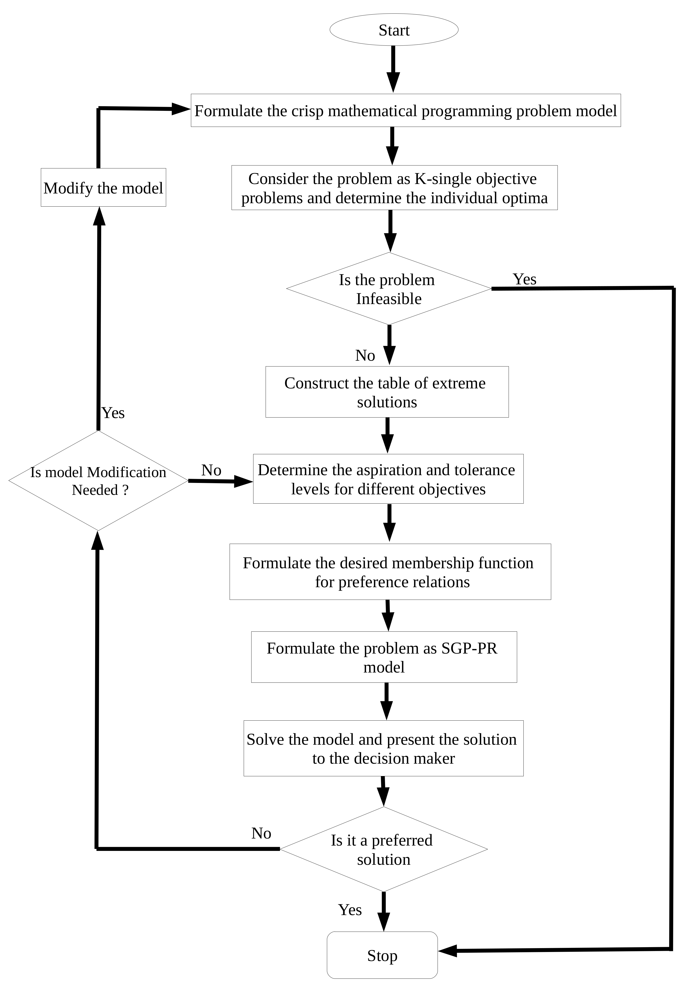
The solution approach to the SGP-PR is consists of multiple steps. Initially, the crisp model of the problem is formulated with all the objectives. Then, to know the best (aspiration) and worst values, either the decision maker is asked or the crisp model is solved individually for each objective function. To proceed further, the solution obtained should be feasible. Take the optimum value as the aspiration value of the objective function. Then, determine all the objective function values for the obtained solution. This will provide us with a payoff table (table of extreme solutions), and the values of aspiration and tolerance level. Formulate all the normalized functions for the objective functions. Construct the transform function for linguistic preference relations by using normalized functions of the objective functions. Define the linguistic preference relations among the different goals and formulate the membership grades of the preference relations. It may be linear or exponential; choose the desired function for fuzzy preference relation.

After, formulating all the functions, now, formulate the problem as SGP-PR as Models 1–4, as detailed in the previous section. Solve the formulation using any optimization software package such as LINGO (Schrage and LINDO Systems [48], Tan et al. [49]), NEOS (Server [50]), AMPL (Fourer et al. [51]), etc. For this paper, the obtained mathematical programming problem was modeled in AMPL language (Fourer et al. [51]) and solved using solvers available on NEOS server online facility provided by Wisconsin Institutes for Discovery at the University of Wisconsin in Madison for solving optimization problems (see Server [50], Gropp, W. Moré [52], Czyzyk et al. [53], Dolan [54]).

As the solution is obtained, check the feasibility and optimality. If it is infeasible, stop and repeat the steps by changing the aspiration and tolerance values, If not, present the solution to the DM. The flow chart of the procedure is presented in Figure 4.

4. Experimental Study

To validate and compare the proposed goal programming models, we applied the GP models on a numerical example. The solution approach used is already detailed in previous section. The main focus is on the validity and the performance of the proposed models. We considered a multi-objective mathematical programming problem, which was already used by Aköz and Petrovic [16], Chen and Tsai [18], Cheng [19], and Arenas-Parra et al. [35]:

$$\begin{array}{cc}\hfill \mathrm{Goal}1:& f_1(x):=4x_1+2x_2+8x_3+x_4\le 35,\hfill \end{array}$$

(17a)

$$\begin{array}{cc}\hfill \mathrm{Goal}2:& f_2(x):=4x_1+7x_2+6x_3+2x_4\ge 100,\hfill \end{array}$$

(17b)

$$\begin{array}{cc}\hfill \mathrm{Goal}3:& f_3(x):=x_1-6x_2+5x_3+10x_4\ge 120,\hfill \end{array}$$

(17c)

$$\begin{array}{cc}\hfill \mathrm{Goal}4:& f_4(x):=5x_1+3x_2+2x_4\ge 70,\hfill \end{array}$$

(17d)

$$\begin{array}{cc}\hfill \mathrm{Goal}5:& f_5(x):=4x_1+4x_2+4x_3\ge 40,\hfill \end{array}$$

(17e)

$$\begin{array}{cc}\hfill \mathrm{subject}\mathrm{to}& 7x_1+5x_2+3x_3+2x_4\le 98,\hfill \end{array}$$

(17f)

$$\begin{array}{cc}\hfill & 7x_1+x_2+2x_3+6x_4\le 117,\hfill \end{array}$$

(17g)

$$\begin{array}{cc}\hfill & x_1+x_2+2x_3+6x_4\le 130,\hfill \end{array}$$

(17h)

$$\begin{array}{cc}\hfill & 9x_1+x_2+6x_4\le 105,\hfill \end{array}$$

(17i)

$$\begin{array}{cc}\hfill & x_i\ge 0,i=1,\dots ,4.\hfill \end{array}$$

(17j)

The type of preference relations between the goals are assumed as:

• Goal 1 is significantly more important than Goal 2.
• Goal 2 is significantly more important than Goal 4.
• Goal 2 is significantly more important than Goal 5.
• Goal 3 is fully more important than Goal 2.

The solution steps are as follows:

Step:1 Start

Step:2 The optimization model is formulated as single objective problem and result values are obtained for all the objectives. It will provide us the best and worst values for the objectives.

Solving the numerical example using the software packages for each objective function independently and finding the best and worst value of five objective functions, we get $\underline{f_1}=487.66,f_1^{\ast }=261.33$, $f_2^{\ast }=100,\underline{f_2}=0$, $f_3^{\ast }=120.16,\underline{f_3}=-117.6$, $f_4^{\ast }=70,\underline{f_4}=0$ and $f_5^{\ast }=40,\underline{f_5}=0$. The solution obtained is feasible and optimal.

Step:3 Formulate the normalized function and membership grades for linear and exponential preference relations.

$$n_1=1-{\displaystyle \frac{d_1^{+}}{226.33}},n_2=1-{\displaystyle \frac{d_2^{-}}{100}},n_3=1-{\displaystyle \frac{d_3^{-}}{237.76}},n_4=1-{\displaystyle \frac{d_4^{-}}{70}},n_5=1-{\displaystyle \frac{d_5^{-}}{40}},$$

Membership functions for linear preference relations:

$${\mu }_{{\tilde{R}}_6(1,2)}=\frac{(n_1-n_2+1)}{2},{\mu }_{{\tilde{R}}_6(2,4)}=\frac{(n_2-n_4+1)}{2},$$

$${\mu }_{{\tilde{R}}_6(2,5)}=\frac{(n_2-n_5+1)}{2},{\mu }_{{\tilde{R}}_8(3,2)}=(n_3-n_2)$$

Membership functions for exponential preference relations:

$${\mu }_{{\tilde{R}}_6(1,2)}=1-{\displaystyle \frac{e^{-s·(\frac{n_1-n_2+1}{2})}-e^{-s}}{1-e^{-s}}},{\mu }_{{\tilde{R}}_6(2,4)}=1-{\displaystyle \frac{e^{-s·(\frac{n_2-n_4+1}{2})}-e^{-s}}{1-e^{-s}}},$$

$${\mu }_{{\tilde{R}}_6(2,5)}=1-{\displaystyle \frac{e^{-s·(\frac{n_2-n_5+1}{2})}-e^{-s}}{1-e^{-s}}},{\mu }_{{\tilde{R}}_8(3,2)}=1-{\displaystyle \frac{e^{-s·(n_3-n_2)}-e^{-s}}{1-e^{-s}}}$$

Step:4 Now, formulate the problem as Models 1–4, as detailed in Section 2.2. The formulation of Model 1 becomes:

$$\mathrm{Maximize}Z=\alpha (n_1+n_2+n_3+n_4+n_5)+(1-\alpha )({\mu }_{{\tilde{R}}_6(1,2)}+{\mu }_{{\tilde{R}}_6(2,4)}+{\mu }_{{\tilde{R}}_6(2,5)}+{\mu }_{{\tilde{R}}_8(3,2)}),$$

(18a)

$$\begin{array}{cc}\hfill \mathrm{subject}\mathrm{to}& 4x_1+2x_2+8x_3+x_4+d_1^{-}-d_1^{+}=35,\hfill \end{array}$$

(18b)

$$\begin{array}{cc}\hfill & 4x_1+7x_2+6x_3+2x_4+d_2^{-}-d_2^{+}=100,\hfill \end{array}$$

(18c)

$$\begin{array}{c}{x}_1-6x_2+5x_3+10x_4+d_3^{-}-d_3^{+}=120,\hfill \end{array}$$

(18d)

$$\begin{array}{c}5x_1+3x_2+2x_4+d_4^{-}-d_4^{+}=70,\hfill \end{array}$$

(18e)

$$\begin{array}{c}4x_1+4x_2+4x_3+d_5^{-}-d_5^{+}=40,\hfill \end{array}$$

(18f)

$$\begin{array}{c}{n}_1=1-{\displaystyle \frac{d_1^{+}}{226.33}},n_2=1-{\displaystyle \frac{d_2^{-}}{100}},n_3=1-{\displaystyle \frac{d_3^{-}}{237.76}},\hfill \end{array}$$

(18g)

$$\begin{array}{c}\hfill n_4=1-{\displaystyle \frac{d_4^{-}}{70}},n_5=1-{\displaystyle \frac{d_5^{-}}{40}},\end{array}$$

(18h)

$$\begin{array}{cc}\hfill & \frac{(n_1-n_2+1)}{2}\ge {\mu }_{{\tilde{R}}_6(1,2)},\hfill \end{array}$$

(18i)

$$\begin{array}{cc}\hfill & \frac{(n_2-n_4+1)}{2}\ge {\mu }_{{\tilde{R}}_6(2,4)},\hfill \end{array}$$

(18j)

$$\begin{array}{cc}\hfill & \frac{(n_2-n_5+1)}{2}\ge {\mu }_{{\tilde{R}}_6(2,5)},\hfill \end{array}$$

(18k)

$$\begin{array}{cc}\hfill & (n_3-n_2)\ge {\mu }_{{\tilde{R}}_8(3,2)},\hfill \end{array}$$

(18l)

$$\begin{array}{cc}\hfill & 7x_1+5x_2+3x_3+2x_4\le 98,\hfill \end{array}$$

(18m)

$$\begin{array}{cc}\hfill & 7x_1+x_2+2x_3+6x_4\le 117,\hfill \end{array}$$

(18n)

$$\begin{array}{c}{x}_1+x_2+2x_3+6x_4\le 130,\hfill \end{array}$$

(18o)

$$\begin{array}{c}\hfill 9x_1+x_2+6x_4\le 105,\end{array}$$

(18p)

$$\begin{array}{cc}\hfill & 0\le {\mu }_{{\tilde{R}}_6(1,2)},{\mu }_{{\tilde{R}}_6(2,4)},{\mu }_{{\tilde{R}}_6(2,5)},{\mu }_{{\tilde{R}}_8(3,2)}\le 1,\hfill \end{array}$$

(18q)

$$\begin{array}{cc}\hfill & x_i\ge 0,n_k\ge 0,i=1,\dots ,4,k=1,\dots ,5,\hfill \end{array}$$

(18r)

$$\begin{array}{cc}\hfill & 0\le n_k\le 1,k=1,\dots ,5.\hfill \end{array}$$

(18s)

$$\begin{array}{cc}\hfill & d_k^{-}·d_k^{+}=0,\hfill \end{array}$$

(18t)

$$\begin{array}{cc}\hfill & {\mu }_{\tilde{R}(k,l)}\ge 0\mathrm{for}\mathrm{all}{b}_{kl}=1.\hfill \end{array}$$

(18u)

The formulation for Model 2 becomes the same model as Model 1 with replacement of Equations (18i)–(18l) by Equations (19a)–(19d).

$$\begin{array}{cc}\hfill & 1-{\displaystyle \frac{e^{-s·(\frac{n_1-n_2+1}{2})}-e^{-s}}{1-e^{-s}}}\ge {\mu }_{{\tilde{R}}_6(1,2)},\hfill \end{array}$$

(19a)

$$\begin{array}{c}1-{\displaystyle \frac{e^{-s·(\frac{n_2-n_4+1}{2})}-e^{-s}}{1-e^{-s}}}\ge {\mu }_{{\tilde{R}}_6(2,4)},\hfill \end{array}$$

(19b)

$$\begin{array}{c}1-{\displaystyle \frac{e^{-s·(\frac{n_2-n_5+1}{2})}-e^{-s}}{1-e^{-s}}}\ge {\mu }_{{\tilde{R}}_6(2,5)},\hfill \end{array}$$

(19c)

$$\begin{array}{c}1-{\displaystyle \frac{e^{-s·(n_3-n_2)}-e^{-s}}{1-e^{-s}}}\ge {\mu }_{{\tilde{R}}_8(3,2)},\hfill \end{array}$$

(19d)

The formulation of Model 3 is

$$\mathrm{Maximize}Z={\gamma }_1(\lambda )+{\gamma }_2(n_1+n_2+n_3+n_4+n_5)+{\gamma }_3({\mu }_{{\tilde{R}}_6(1,2)}+{\mu }_{{\tilde{R}}_6(2,4)}+{\mu }_{{\tilde{R}}_6(2,5)}+{\mu }_{{\tilde{R}}_8(3,2)}),$$

(20a)

$$\begin{array}{cc}\hfill \mathrm{subject}\mathrm{to}& \lambda \le n_1,n_2,n_3,n_4,n_5,\hfill \end{array}$$

(20b)

$$\begin{array}{cc}\hfill & (18\mathsf{b})–(18\mathsf{u})\hfill \end{array}$$

(20c)

The formulation for Model 4 is as follows:

$$\mathrm{Maximize}Z={\gamma }_1(\lambda )+{\gamma }_2(n_1+n_2+n_3+n_4+n_5)+{\gamma }_3({\mu }_{{\tilde{R}}_6(1,2)}+{\mu }_{{\tilde{R}}_6(2,4)}+{\mu }_{{\tilde{R}}_6(2,5)}+{\mu }_{{\tilde{R}}_8(3,2)}),$$

(21a)

$$\begin{array}{cc}\hfill \mathrm{subject}\mathrm{to}& \lambda \le n_1,n_2,n_3,n_4,n_5,\hfill \end{array}$$

(21b)

$$\begin{array}{cc}\hfill & (18\mathsf{b})–(18\mathsf{h})\hfill \end{array}$$

(21c)

$$\begin{array}{cc}\hfill & (19\mathsf{a})–(19\mathsf{d})\hfill \end{array}$$

(21d)

$$\begin{array}{cc}\hfill & (18\mathsf{m})–(18\mathsf{u})\hfill \end{array}$$

(21e)

Step:5 As the formulation is done, then all the models are modeled in AMPL language (Fourer et al. [51]) and solved by the CONOPT solver (Drud [55]) using the NEOS server online facility provided by Wisconsin Institutes for Discovery at the University of Wisconsin in Madison for solving Optimization problems (see Gropp, W. Moré [52], Czyzyk et al. [53], Dolan [54], and Server [50]). The solution obtained is feasible and optimal.

Step:6 The method is stopped and the solution is presented to the DM.

4.1. Results and Discussion

The results obtained by formulating and solving Models 1–4 on the numerical example are presented in

Table 2. Solution results for Model 1 (Linear).

Variables	Model 1 (Linear)
$\mathit{\alpha }$	0	0.1	0.2	0.3	0.4	0.5	0.6	0.7	0.8	0.9	1
Z	2.7085	2.696	2.6834	2.67086	2.8468	3.1662	3.486	3.8059	4.1257	4.4456	4.7655
$f_1$	12	12	12	12	45.9139	46.3816	46.3816	46.3816	46.3816	46.3816	46.3816
$f_2$	24	24	24	24	100	100.526	100.526	100.526	100.526	100.526	100.526
$f_3$	120	120	120	120	120	120	120	120	120	120	120
$f_4$	24	24	24	24	57.0168	57.1053	57.1053	57.1053	57.1053	57.1053	57.1053
$f_5$	0	0	0	0	39.6639	40	40	40	40	40	40
$x_1$	0	0	0	0	0	0	0	0	0	0	0
$x_2$	0	0	0	0	8.2563	8.2894	8.2894	8.2894	8.2894	8.2894	8.2894
$x_3$	0	0	0	0	1.6596	1.7105	1.7105	1.7105	1.7105	1.7105	1.7105
$x_4$	12	12	12	12	16.1239	16.1184	16.1184	16.1184	16.1184	16.1184	16.1184
$n_1$	1	1	1	1	0.9517	0.9497	0.9497	0.9497	0.9497	0.9497	0.9497
$n_2$	0.24	0.24	0.24	0.24	1	1	1	1	1	1	1
$n_3$	1	1	1	1	1	1	1	1	1	1	1
$n_4$	0.3428	0.3428	0.3428	0.3428	0.8145	0.8157	0.8157	0.8157	0.8157	0.8157	0.8157
$n_5$	0	0	0	0	0.9915	1	1	1	1	1	1
${\mu }_{12}$	0.88	0.88	0.88	0.88	0.4758	0.4748	0.4748	0.4748	0.4748	0.4748	0.4748
${\mu }_{24}$	0.4485	0.4485	0.4485	0.4485	0.5927	0.5921	0.5921	0.5921	0.592105	0.5921	0.5921
${\mu }_{32}$	0.76	0.76	0.76	0.76	0	0	0	0	0	0	0
${\mu }_{25}$	0.62	0.62	0.62	0.62	0.5042	0.5	0.5	0.5	0.5	0.5	0.5
$\sum n_k$	2.5828	2.5828	2.5828	2.5828	4.7579	4.7655	4.7655	4.7655	4.7655	4.7655	4.7655
$\sum {\mu }_{R_q}(k,l)$	2.7085	2.7085	2.7085	2.7085	1.5728	1.5669	1.5669	1.5669	1.5669	1.5669	0

,

Table 3. Solution results for Model 2 (Exponential).

Variables	Model 2 (Exponential)
$\alpha$	0	0.1	0.2	0.3	0.4	0.5	0.6	0.7	0.8	0.9	1
Z	3.0707	3.0219	2.9731	2.9474	3.0969	3.3464	3.6302	3.914	4.1978	4.4816	4.7655
$f_1$	12	12	12	35	35	46.3816	46.3816	46.3816	46.3816	46.3816	46.3816
$f_2$	24	24	24	45.7463	84.8031	100.526	100.526	100.526	100.526	100.526	100.526
$f_3$	120	120	120	134.416	120	120	120	120	120	120	120
$f_4$	24	24	24	27.1662	54.1798	57.1053	57.1053	57.1053	57.1053	57.1053	57.1053
$f_5$	0	0	0	13.3127	31.0515	40	40	40	40	40	40
$x_1$	0	0	0	0	0.2852	0	0	0	0	0	0
$x_2$	0	0	0	0.6944	6.9784	8.2894	8.2894	8.2894	8.2894	8.2894	8.2894
$x_3$	0	0	0	2.6337	0.4991	1.7105	1.7105	1.7105	1.7105	1.7105	1.7105
$x_4$	12	12	12	12.5414	15.909	16.1184	16.1184	16.1184	16.1184	16.1184	16.1184
$n_1$	1	1	1	1	1	0.9497	0.9497	0.9497	0.9497	0.9497	0.9497
$n_2$	0.24	0.24	0.24	0.4574	0.848	1	1	1	1	1	1
$n_3$	1	1	1	1	1	1	1	1	1	1	1
$n_4$	0.3428	0.3428	0.3428	0.3880	0.7739	0.8157	0.8157	0.8157	0.8157	0.8157	0.8157
$n_5$	0	0	0	0.3328	0.7762	1	1	1	1	1	1
${\mu }_{12}$	0.9258	0.9258	0.9258	0.8504	0.6926	0.598	0.5980	0.5980	0.5980	0.5980	0
${\mu }_{24}$	0.5718	0.5718	0.5718	0.6551	0.6573	0.7068	0.7068	0.7068	0.7068	0.7068	0
${\mu }_{32}$	0.8421	0.8421	0.8421	0.6624	0.223	0	0	0	0	0	0
${\mu }_{25}$	0.7309	0.7309	0.7309	0.6804	0.6562	0.6224	0.6224	0.6224	0.6224	0.6224	0
$\sum n_k$	2.5828	2.5828	2.5828	3.1783	4.3983	4.7655	4.7655	4.7655	4.7655	4.7655	4.7655
$\sum {\mu }_{R_q}(k,l)$	3.0707	3.0707	3.0707	2.8484	2.2293	1.9273	1.9273	1.9273	1.9273	1.9273	0

,

Table 4. Solution results for Model 3 (Linear).

Variables	Model 3 (Linear)
(${\mathit{\gamma }}_{\mathbf{1}},{\mathit{\gamma }}_{\mathbf{2}},{\mathit{\gamma }}_{\mathbf{3}}$)	c1	c2	c3	c4	c5	c6
Z	2.4251	2.4785	4.0506	2.1444	2.9408	2.0899
$f_1$	12	35	46.3816	46.3816	46.3816	65.1907
$f_2$	24	87.7187	100.526	100.526	100.526	121.692
$f_3$	120	120	120	120	120	120
$f_4$	24	54.9527	57.1053	57.1053	57.1053	60.6625
$f_5$	0	31.8203	40	40	40	53.5177
$x_1$	0	0	0	0	0	0
$x_2$	0	7.4822	8.2894	8.2894	8.2894	9.62345
$x_3$	0	0.4728	1.7105	1.7105	1.7105	3.7559
$x_4$	12	16.253	16.1184	16.1184	16.1184	15.8961
$\lambda$	0	0.7850	0.8157	0.8157	0.8157	0.8666
$n_1$	1	1	0.9497	0.9497	0.9497	0.8666
$n_2$	0.24	0.8771	1	1	1	1
$n_3$	1	1	1	1	1	1
$n_4$	0.3428	0.7850	0.8157	0.8157	0.8157	0.8666
$n_5$	0	0.7955	1	1	1	1
${\mu }_{12}$	0.88	0.5614	0.4748	0.4748	0.4748	0.4333
${\mu }_{24}$	0.4485	0.5460	0.5921	0.5921	0.5921	0.5666
${\mu }_{32}$	0.76	0.1228	0	0	0	0
${\mu }_{25}$	0.62	0.5408	0.5	0.5	0.5	0.5
$\sum n_k$	2.5828	4.4577	4.7655	4.7655	4.7655	4.7332
$\sum {\mu }_{R_q}(k,l)$	2.7085	1.7711	1.5669	1.5669	1.5669	1.5

and

Table 5. Solution results for Model 4 (Exponential).

Variables	Model 4 (Exponential)
(${\mathit{\gamma }}_{\mathbf{1}},{\mathit{\gamma }}_{\mathbf{2}},{\mathit{\gamma }}_{\mathbf{3}}$)	c1	c2	c3	c4	c5	c6
Z	2.7148	2.7444	4.0867	2.2526	3.0129	2.1262
$f_1$	12	35	46.3816	46.3816	46.3816	65.1907
$f_2$	24	70.4306	100.526	100.526	100.526	121.692
$f_3$	120	120	120	120	120	120
$f_4$	24	50.3698	57.1053	57.1053	57.1053	60.6625
$f_5$	0	27.2614	40	40	40	53.5177
$x_1$	0	1.6916	0	0	0	0
$x_2$	0	4.4949	8.2894	8.2894	8.2894	9.6234
$x_3$	0	0.6287	1.7105	1.7105	1.7105	3.7559
$x_4$	12	14.2134	16.1184	16.1184	16.1184	15.8961
$\lambda$	0	0.6815	0.8157	0.8157	0.8157	0.8666
$n_1$	1	1	0.9497	0.9497	0.9497	0.8666
$n_2$	0.24	0.7043	1	1	1	1
$n_3$	1	1	1	1	1	1
$n_4$	0.3428	0.7195	0.8157	0.8157	0.8157	0.8666
$n_5$	0	0.6815	1	1	1	1
${\mu }_{12}$	0.9258	0.7543	0.5980	0.5980	0.5980	0.5562
${\mu }_{24}$	0.5718	0.6151	0.7068	0.7068	0.7068	0.6843
${\mu }_{32}$	0.8421	0.4049	0	0	5.38E-17	0
${\mu }_{25}$	0.7309	0.6333	0.6224	0.6224	0.6224	0.6224
$\sum n_k$	2.5828	4.1054	4.7655	4.7655	4.7655	4.7332
$\sum {\mu }_{R_q}(k,l)$	3.0707	2.4077	1.9273	1.9273	1.9273	1.8631

, respectively. To analyze the result in more detail, multiple values of weight parameter $\alpha$ and (${\gamma }_1,{\gamma }_2,{\gamma }_3$) are considered. The decision maker is free to choose these weight parameters $\alpha$ and (${\gamma }_1,{\gamma }_2,{\gamma }_3$), such that ${\gamma }_1+{\gamma }_2+{\gamma }_3=1$ in between 0 snf 1. Ten cases of $\alpha$ and six cases of weight combinations for (${\gamma }_1,{\gamma }_2,{\gamma }_3$) as c1 = ( 0.1,0.1,0.8), c2 = ( 0.1,0.3,0.6), c3 = ( 0.1,0.8,0.1), c4 = ( 0.3,0.3,0.3), c5 = ( 0.3,0.5,0.2), and c6 = ( 0.6,0.3,0.1) on his/her preferences are considered.

On solving models, many result values for normalized function, decision variables, individual objective function, and membership grade of preference relations between the multiple objectives are obtained. The detailed result values are presented in Table 2, Table 3, Table 4 and Table 5.

In Table 2 and Table 3, the value of $\sum n_k$ is increasing and for $\sum {\mu }_{R_q}(k,l)$ is decreasing from $\alpha$ = 0 to 1. In Table 2, the values for $\sum n_k$ are the same for $\alpha =$ 0–0.3 as 2.5828 and $\alpha =$ 0.5–1 as 4.7655. In Table 3, the values of $\sum n_k$ for $\alpha =$ 0–0.2 and $\alpha =$ 0.5–1 are same as Model 1. For all the values of $\sum {\mu }_{R_q}(k,l)$, Model 2 is higher and thus better than Model 1 for all values of $\alpha$.

In addition, all decision variables of Table 2, Table 3, Table 4 and Table 5 for Models 3 and 4 present one more decision variable $\lambda$, which is the minimum value of the normalized function ($n_k$) among all the objective functions $f_k$. Table 4 and Table 5 present the solution values of Models 3 and 4, respectively. On comparing Models 3 and 4, for $\sum n_k$ and $\sum {\mu }_{R_q}(k,l)$, we find that Model 4 performs better than Model 3 for all cases of (${\gamma }_1,{\gamma }_2,{\gamma }_3$). The value of $\sum n_k$ is the same for c1, c3, c4, c5, and c6 for Models 3 and 4, whereas $\sum {\mu }_{R_q}{(k,l)}_{Model4}>\sum {\mu }_{R_q}{(k,l)}_{Model3}$ for all combinations of (${\gamma }_1,{\gamma }_2,{\gamma }_3$). In the case of c2, $\sum n_k$ of Model 4 has a higher value than Model 3.

To get more insight into the analysis of Models 1–4 with linear and exponential preference relations, we further solved the numerical example for five types of preference relations combinations. The considered preference relation types are as follows:

Preference Relation Type-1 (PRT-1):

The preference relations between the goals are:

• Goal 1 is significantly more important than Goal 2.
• Goal 2 is significantly more important than Goal 4.
• Goal 2 is significantly more important than Goal 5.
• Goal 3 is fully more important than Goal 2.

Preference Relation Type-2 (PRT-2):

The preference relations between the goals are:

• Goal 1 is significantly more important than Goal 2.
• Goal 2 is significantly more important than Goal 4.
• Goal 2 is significantly more important than Goal 5.
• Goal 3 is significantly more important than Goal 2.

Preference Relation Type-3 (PRT-3):

The preference relations between the goals are:

• Goal 1 is significantly more important than Goal 2.
• Goal 2 is partially equal to Goal 4.
• Goal 2 is significantly more important than Goal 5.
• Goal 3 is fully more important than Goal 2.

Preference Relation Type-4 (PRT-4):

The preference relations between the goals are:

• Goal 1 is significantly more important than Goal 2.
• Goal 2 is completely more important than Goal 4.
• Goal 2 is moderately more important than Goal 5.
• Goal 3 is fully more important than Goal 2.

Preference Relation Type-5 (PRT-5):

The preference relations between the goals are:

• Goal 1 is significantly more important than Goal 2.
• Goal 2 is significantly more important than Goal 4.
• Goal 2 is significantly more important than Goal 5.
• Goal 3 is partially more important than Goal 2.

A total of twenty five different models are formulated. After modeling and solving the problem models, the results are presented in

Table 6. Solution results of Model 1 (Linear) for all cases of preference relations.

PR Type	Model 1 (Linear)
	$\mathit{\alpha }$	0	0.1	0.2	0.3	0.4	0.5	0.6	0.7	0.8	0.9	1
PRT1	$\sum n_k$	2.5828	2.5828	2.5828	2.5828	4.7579	4.7655	4.7655	4.7655	4.7655	4.7655	4.7655
	$\sum {\mu }_{R_q}(k,l)$	2.7085	2.7085	2.7085	2.70857	1.5728	1.5669	1.56696	1.56696	1.56696	1.56696	0
PRT2	$\sum n_k$	2.5828	4.4577	4.4577	4.4577	4.7579	4.7655	4.7655	4.7655	4.786	4.786	4.786
	$\sum {\mu }_{R_q}(k,l)$	2.8285	2.2097	2.2097	2.2097	2.0728	2.0669	2.0669	2.0669	2.012	2.012	0
PRT3	$\sum n_k$	2.8	2.8	2.8	2.8	4.1554	4.1554	4.6364	4.7655	4.7655	4.7655	4.7655
	$\sum {\mu }_{R_q}(k,l)$	3.1	3.1	3.1	3.1	2.4222	2.4222	1.8249	1.6064	1.6064	1.6064	0
PRT4	$\sum n_k$	2.5828	2.5828	2.5828	2.5828	4.7579	4.7655	4.7655	4.7655	4.7655	4.7655	4.7655
	$\sum {\mu }_{R_q}(k,l)$	2.7314	2.7314	2.7314	2.7314	1.6051	1.5976	1.5976	1.5976	1.5976	1.5976	0
PRT5	$\sum n_k$	1.4949	2.85	4.7616	4.7616	4.7616	4.786	4.786	4.786	4.786	4.786	4.786
	$\sum {\mu }_{R_q}(k,l)$	3	2.925	2.5759	2.5759	2.5759	2.5576	2.5576	2.5576	2.5576	2.5576	0

,

Table 7. Solution results of Model 2 (Exponential) for all cases of preference relations.

PR Type	Model 2 (Exponential)
	$\mathit{\alpha }$	0	0.1	0.2	0.3	0.4	0.5	0.6	0.7	0.8	0.9	1
PRT1	$\sum n_k$	2.5828	2.5828	2.5828	3.17837	4.3983	4.7655	4.7655	4.7655	4.7655	4.7655	4.7655
	$\sum {\mu }_{R_q}(k,l)$	3.0707	3.0707	3.0707	2.84845	2.2293	1.9273	1.92737	1.92737	1.92737	1.92737	0
PRT2	$\sum n_k$	2.5828	2.5828	3.2	4.5716	4.7579	4.7655	4.7655	4.7655	4.786	4.786	4.786
	$\sum {\mu }_{R_q}(k,l)$	3.1543	3.1543	3.0372	2.6378	2.5554	2.5498	2.5498	2.5498	2.4987	2.4987	0
PRT3	$\sum n_k$	2.7526	2.8	2.8	3.1477	4.1554	4.1554	4.7655	4.7655	4.7655	4.7655	4.7655
	$\sum {\mu }_{R_q}(k,l)$	3.3765	3.3757	3.3757	3.2372	2.757	2.757	1.9612	1.9612	1.9612	1.9612	0
PRT4	$\sum n_k$	2.5828	2.5828	2.8261	3.1876	4.4577	4.7655	4.7655	4.7655	4.7655	4.7655	4.7655
	$\sum {\mu }_{R_q}(k,l)$	3.0257	3.0257	2.9734	2.8471	2.1912	1.9472	1.9472	1.9472	1.9472	1.9472	0
PRT5	$\sum n_k$	1.4949	3.2	4.7616	4.7616	4.7616	4.786	4.786	4.786	4.786	4.786	4.786
	$\sum {\mu }_{R_q}(k,l)$	3.2449	3.1955	2.9382	2.9382	2.9382	2.921	2.921	2.921	2.921	2.921	0

,

Table 8. Solution results of Model 3 (Linear) for all cases of preference relations.

	Variables	Model 3 (Linear)
PR Type	(${\mathit{\gamma }}_{\mathbf{1}},{\mathit{\gamma }}_{\mathbf{2}},{\mathit{\gamma }}_{\mathbf{3}}$)	c1	c2	c3	c4	c5	c6
PRT1	$\sum n_k$	2.5828	4.4577	4.7655	4.7655	4.7655	4.7332
	$\sum {\mu }_{R_q}(k,l)$	2.7085	1.77113	1.5669	1.5669	1.5669	1.5
PRT2	$\sum n_k$	2.5828	4.7579	4.786	4.786	4.7851	4.7556
	$\sum {\mu }_{R_q}(k,l)$	2.8285	2.0728	2.012	2.012	1.9965	1.9592
PRT3	$\sum n_k$	2.8	4.1554	4.7655	4.4987	4.7332	4.7332
	$\sum {\mu }_{R_q}(k,l)$	3.1	2.4222	1.6064	2.0085	1.6665	1.6665
PRT4	$\sum n_k$	2.5828	4.4577	4.7655	4.7655	4.7655	4.7655
	$\sum {\mu }_{R_q}(k,l)$	2.7314	1.8001	1.5976	1.5976	1.5976	1.5976
PRT5	$\sum n_k$	3.2	4.7616	4.786	4.7851	4.7851	4.7851
	$\sum {\mu }_{R_q}(k,l)$	2.8812	2.5759	2.5576	2.5485	2.5485	2.5485

, and

Table 9. Solution results for Model 4 (Exponential) for all cases of preference relations.

	Variables	Model 4 (Exponential)
PR Type	(${\mathit{\gamma }}_{\mathbf{1}},{\mathit{\gamma }}_{\mathbf{2}},{\mathit{\gamma }}_{\mathbf{3}}$)	c1	c2	c3	c4	c5	c6
PRT1	$\sum n_k$	2.5828	4.1054	4.7655	4.7655	4.7655	4.7332
	$\sum {\mu }_{R_q}(k,l)$	3.0707	2.4077	1.9273	1.9273	1.9273	1.8631
PRT2	$\sum n_k$	2.99	4.7579	4.786	4.786	4.7851	4.7556
	$\sum {\mu }_{R_q}(k,l)$	3.0787	2.5554	2.4987	2.4987	2.4839	2.4483
PRT3	$\sum n_k$	4.7154	4.7174	4.7655	4.7332	4.7332	4.7332
	$\sum {\mu }_{R_q}(k,l)$	2.0184	2.0165	1.9612	2.0008	2.0008	2.0008
PRT4	$\sum n_k$	2.7121	4.097	4.7655	4.7655	4.7655	4.7332
	$\sum {\mu }_{R_q}(k,l)$	3.0001	2.4024	1.9472	1.9472	1.9472	1.8709
PRT5	$\sum n_k$	4.4126	4.7616	4.786	4.7851	4.7851	4.7835
	$\sum {\mu }_{R_q}(k,l)$	3.0136	2.9382	2.921	2.9126	2.9126	2.91

. The values of $\sum n_k$ and $\sum {\mu }_{R_q}(k,l)$ are determined for each preference relation combination on Models 1–4. The values of $\sum n_k$ is increasing while $\sum {\mu }_{R_q}(k,l)$ is decreasing from $\alpha =$0 to 1 for all PR type in Models 1 and 2. In both models, at $\alpha =$ 0, the value of $\sum n_k$ is the same for PRT-1, -2, and -4 as 2.5828, whereas, at $\alpha =$ 1, it is teh same for PRT-1, -3, and -4 as 4.7655 and PRT-2 and -5 as 4.786. The value of $\sum {\mu }_{R_q}(k,l)$ is 0 for all PR Type. On comparing the preference relation membership grades ($\sum {\mu }_{R_q}(k,l)$) for Models 1 and 2 for all PR types, Model 2 performs best.

For Model 3, in c1 the value of $\sum n_k$ is the same for PRT1, -2, and -4. The highest value is for PRT5 at 3.2. In Model 4, for c1 all the values are greater than the values of Model 3. For Model 3, c2 has the value of 4.4577 for PRT1 and 04 but in Model 4 PRT1 and 04 have lesser values compared to Model 3. For c3, all the values in Models 3 and 4 are the same from PRT1–5. The highest one is for c5 as 4.7616. For c4, all the PRTs have same values for Models 3 and 4, except for PRT3 the value is different. For c4, all the values of Models 3 and 4 are same, but for c5 only PRT4 and -5 values are different.

If we compare $\sum {\mu }_{R_q}(k,l)$ for Models 3 and 4, most of the values for Model 4 for all weights combinations are greater than the values of Model 3. Although the decision can be taken based on the requirement by the decision maker.

4.2. Efficiency Analysis

The proposed models were applied to solve the numerical problem with different types of preference relations combinations. The problem models are linear and nonlinear programming models. While solving the models, we found that the solution time is in seconds for both linear and nonlinear models. The computational time has been found acceptable.

Here, Models 1 and 3 and Models 2 and 4 consist of linear and exponential type of preference relations, respectively. We have previously analyzed the models based on values of $\sum n_k$ and $\sum {\mu }_{R_q}(k,l)$ which is not a good basis for analyzing the efficiency and performance of proposed models. Thus, to determine the efficiency of different models, we determine the degree of closeness of the solution value to the ideal solution. For this the concept of distance function is utilized, see the works of Pramanik and Roy [56], Zheng et al. [57], and Zhao et al. [58]. In this paper, a new distance function is developed to select the priority solution for the proposed models.

$$D(x)={(\sum _k^{}{(1-n_k)}^2+\sum _q^{}{(1-{\mu }_{R_q}(k,l))}^2)}^{1/2}$$

(22)

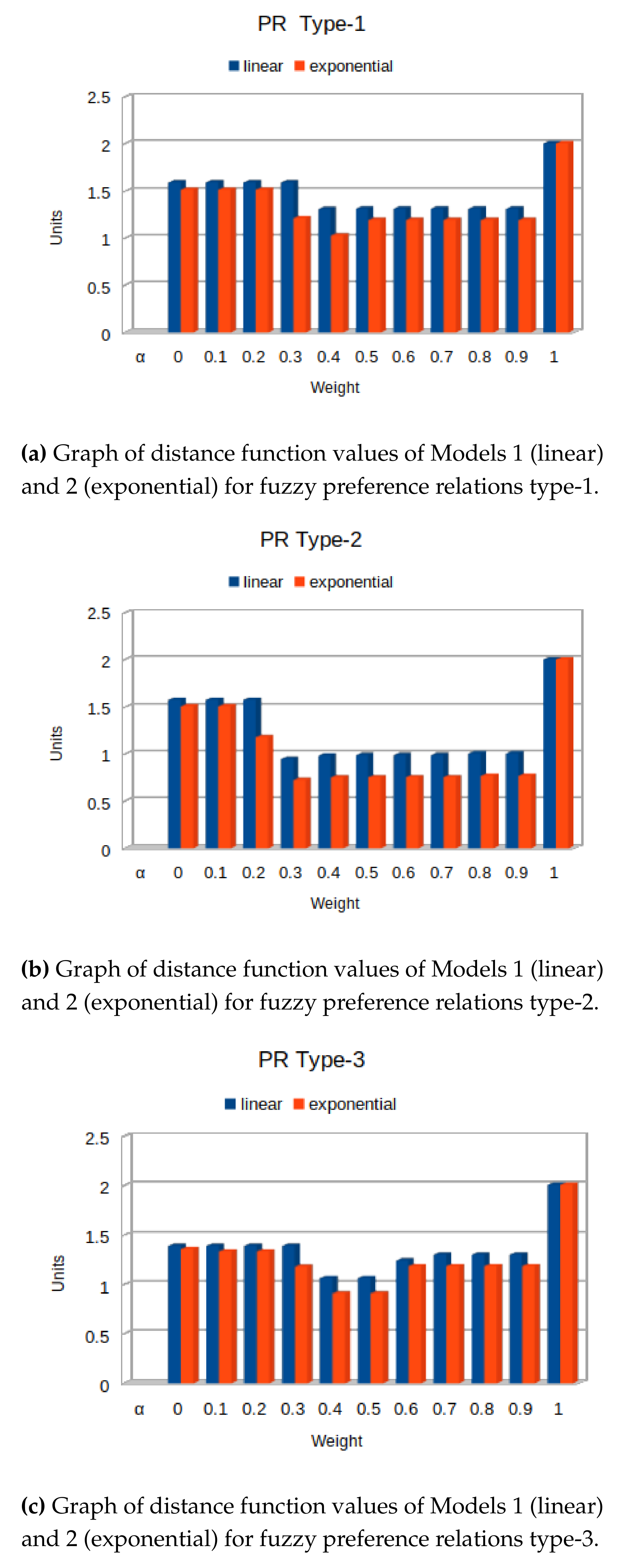
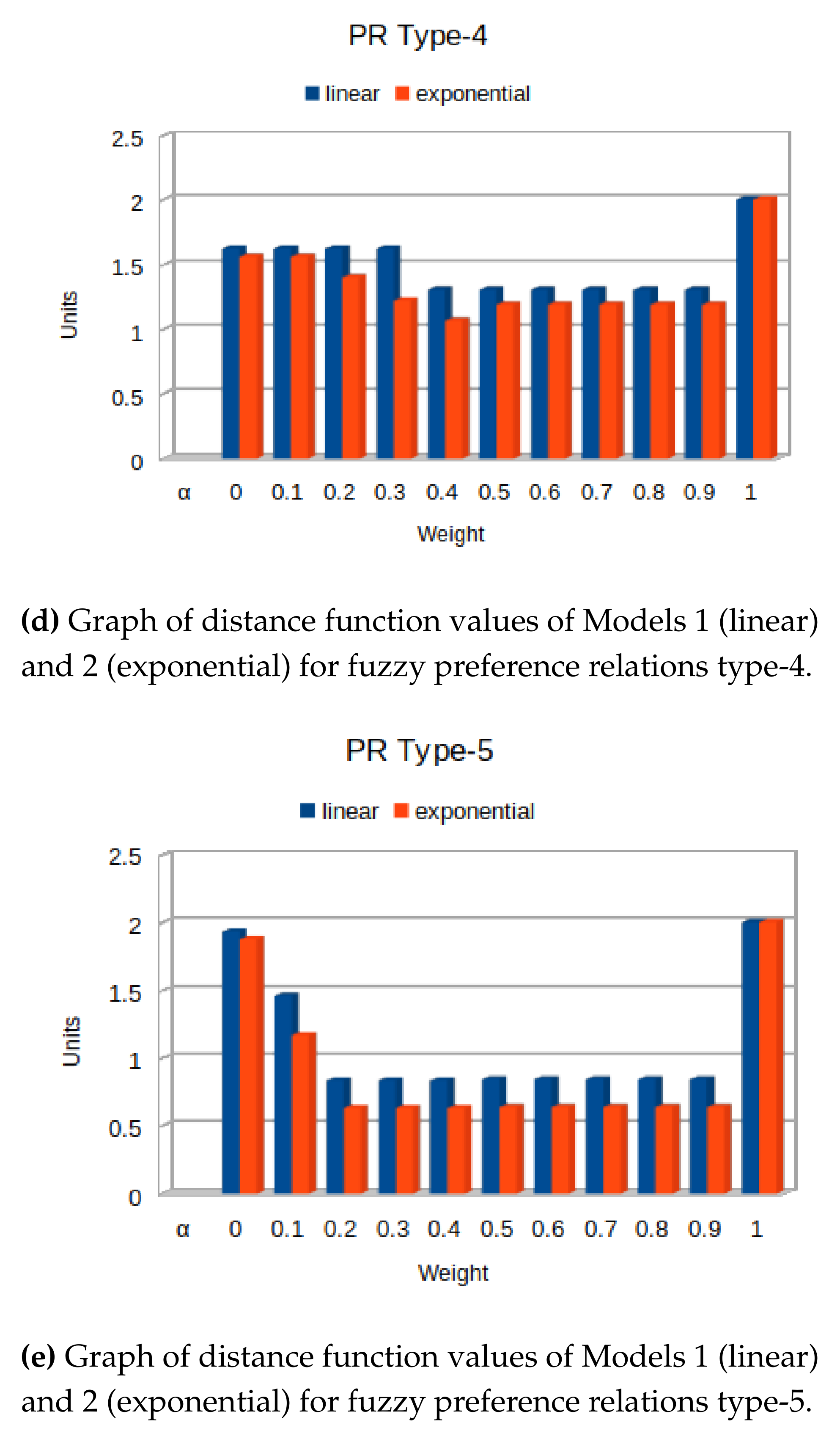
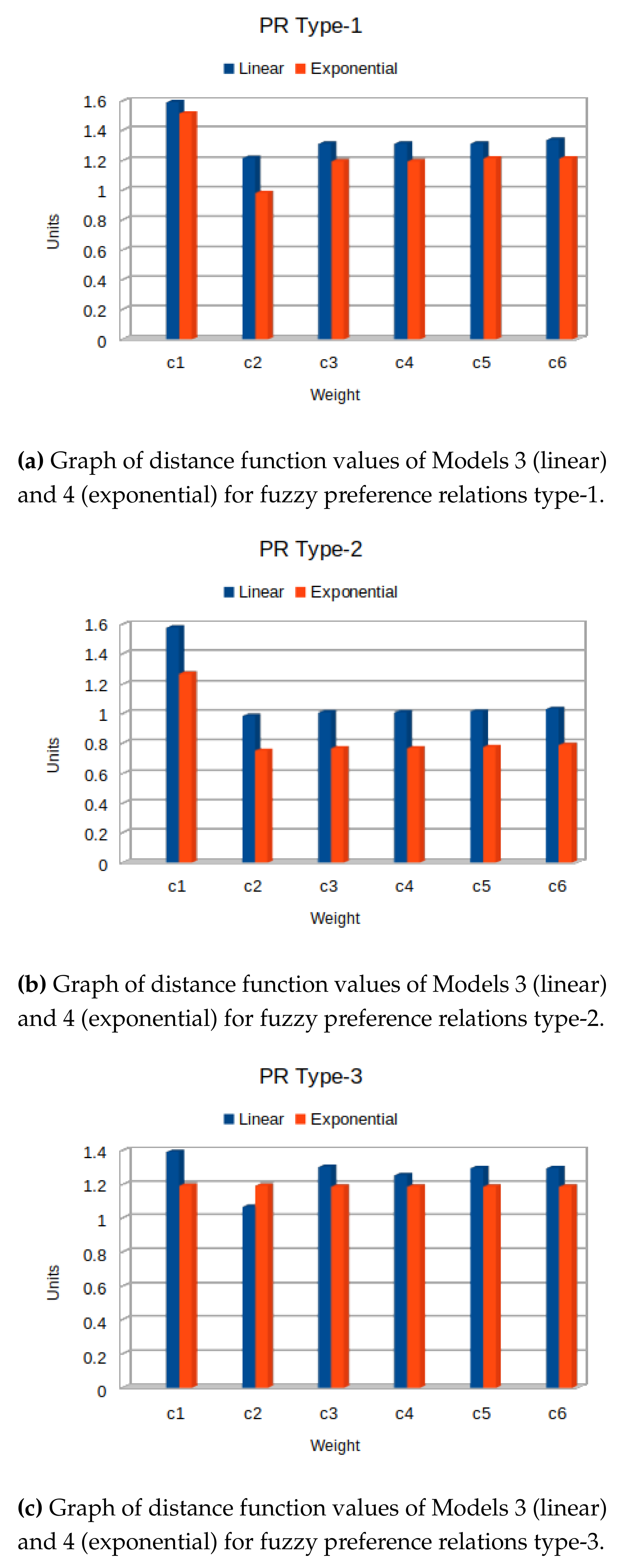
The smaller value of the distance function gives the most satisfying solution as it represents the better solution among all other solutions. The results of numerical example for the distance function is presented in

Table 10. Solution results for distance measure for Models 1 and 2.

PR Type	Distance Measure for Model 1 and 2
	$\mathit{\alpha }$	0	0.1	0.2	0.3	0.4	0.5	0.6	0.7	0.8	0.9	1
PRT1	Model 1	1.5905	1.5905	1.5905	1.5905	1.3126	1.3147	1.3147	1.3147	1.3147	1.3147	2.009
	Model 2	1.5151	1.5151	1.5151	1.2129	1.0285	1.1943	1.1943	1.1943	1.1943	1.1943	2.009
PRT2	Model 1	1.5769	1.5769	1.5769	0.9511	0.9864	0.9892	0.9892	0.9892	1.0079	1.0079	2.0056
	Model 2	1.5087	1.5087	1.1816	0.7274	0.7518	0.7543	0.7543	0.7543	0.7687	0.7687	2.0056
PRT3	Model 1	1.3909	1.3909	1.3909	1.3909	1.0663	1.0663	1.2424	1.303	1.303	1.303	2.009
	Model 2	1.3591	1.3345	1.3345	1.1789	0.9084	0.9084	1.1865	1.1865	1.1865	1.1865	2.009
PRT4	Model 1	1.6285	1.6285	1.6285	1.6285	1.3091	1.3111	1.3111	1.3111	1.3111	1.3111	2.009
	Model 2	1.5657	1.5657	1.4032	1.2258	1.069	1.1949	1.1949	1.1949	1.1949	1.1949	2.009
PRT5	Model 1	1.9378	1.4626	0.838	0.838	0.838	0.8475	0.8475	0.8475	0.8475	0.8475	2.0056
	Model 2	1.8815	1.171	0.6339	0.6339	0.6339	0.6423	0.6423	0.6423	0.6423	0.6423	2.0056

and

Table 11. Solution results for distance measure for Models 3 and 4.

PR Type	Distance Measure for Model 3 and 4
	(${\mathit{\gamma }}_{\mathbf{1}},{\mathit{\gamma }}_{\mathbf{2}},{\mathit{\gamma }}_{\mathbf{3}}$)	c1	c2	c3	c4	c5	c6
PRT1	Model 3	1.5905	1.2172	1.3147	1.3147	1.3147	1.3395
	Model 4	1.5151	0.982	1.1943	1.1943	1.2143	1.2143
PRT2	Model 3	1.5769	0.9864	1.0079	1.0079	1.0151	1.0322
	Model 4	1.2682	0.7518	0.7687	0.7687	0.7754	0.7912
PRT3	Model 3	1.3909	1.0663	1.303	1.2545	1.2953	1.2953
	Model 4	1.1928	1.1918	1.1865	1.186	1.186	1.186
PRT4	Model 3	1.6285	1.2284	1.3111	1.3111	1.3111	1.3422
	Model 4	1.4763	1.0258	1.1949	1.1949	1.1949	1.2217
PRT5	Model 3	1.258	0.838	0.8475	0.8519	0.8519	0.8519
	Model 4	0.6669	0.6339	0.6423	0.6461	0.6461	0.6472

and Figure 5 and Figure 6.

Furthermore, the proposed approach in Models 1 and 2 considers a utility function divided into two criteria: (1) sum of individual normalized function; and (2) sum of membership function for the achievement level of preference relations. Based on these two criteria with a different value of $\alpha$, the performance of different models with five different combinations of preference relations is analyzed. The proposed approach of Models 3 and 4 considers a different and new utility function with addition of maximization of $\lambda$, i.e., minimum value among all the normalized functions. Models 1 and 3 consider membership function for linear preference relations, whereas Models 2 and 4 consider membership function for Exponential preference relation.

In Table 10 and Figure 5, the results for distance function values are shown for different values of $\alpha$ and for type of preference relation model. In Figure 5, it can be seen that for all models of PRT-1–5, Model 2 performs best for all values of $\alpha$. In PRT-2 and -5, the difference of values for Models 1 and 2 is slightly greater than for PRT-1, -3, and -5. For PRT-1 and -4, at $\alpha =0.3$, the difference is more in between Model 1 and 2 for distance function values. It can be seen that, for PRT-5, at $\alpha =$ 0.1–−0.3, the performance of model is best among all other models. It gives the lowest value, 0.838 and 0.6339 for linear and exponential cases, respectively.

In Table 11 and Figure 6, the results for distance function values are shown for different values of $({\gamma }_1,{\gamma }_2,{\gamma }_3)$ and for type of preference relation model. For PRT-1, -2, -4, and -5, Model 4 with exponential preference relation performs best. In the case of PRT-3 for c2, Model 3 is better than Model 4; for the rest of the weight combinations Model 4 is better than Model 3. For PRT-5, the distance function values at c2 is the lowest among all distance function values for different types of preference relations. Overall, the performance ranking is $Model2>Model1$ and $Model4>Model3$. Thus, We can conclude that, for the given experimental study, the performance pattern for the type of membership function is $Exponential>Linear$. For both examples, the results show that the proposed models perform best for the exponential case in comparison to the linear one.

5. Conclusions, Limitations, and Future Directions

This work proposes standard goal programming models with fuzzy hierarchies between the goals. This work is based on several existing methods (see, [16,30,35,38]) and provides an extension to the existing methods by introducing exponential fuzzy preference relations and incorporating new objective function. The exponential membership function for fuzzy preference relations of ten types of linguistic terms is formulated. Four models, namely Models 1–4, based on linear, exponential preference relations, and a new objective are proposed. A numerical example is solved and results are analyzed. A comparison is also made using a newly developed distance measure function for the proposed models to analyze the performance of the proposed models.

It is concluded that, for the experimental numerical problem, solutions are better in case of models having exponential membership function for preference relations in comparison to linear. The proposed models perform better than Model 1, which was proposed by Arenas-Parra et al. [35]. Thus, the efficiency of models with respect to the satisfaction level of the decision maker can be ordered as $Model2>Model1$ and $Model4>Model3$. Another flexibility in the proposed models is that the solution can be chosen according to the priority of the minimum normalized value, the sum of normalized values, and the sum of membership functions of the preference relations. That is, the decision maker can adopt the best solution by having a sensitivity analysis of weight parameters. On choosing the weight ${\gamma }_1=0$, Models 3 and 4 are reduced to Models 1 and 2, respectively.

This study also hase some limitations. As, the results are presented for a single numerical example under different scenarios of preference relations. Further investigation on multiple numerical examples and real life problems are needed to verify the superiority of proposed linear and nonlinear models. The results may change as per the consideration of type of linear and nonlinear preference relations. This research can be extended by the implementation in real life problems from industry such as in scheduling, planning, transportation, manufacturing, supply chain, etc., which can be a challenging work. The inclusion of exponential preferences provides wider applicability in real life scenario. The present work can be further extended to advanced goal programming models using fuzzy, stochastic uncertainties, and different nonlinear membership functions such parabolic, hyperbolic, S-curve, etc. for preference relations.

References

1. Hwang, C.L.; Masud, A.S.M. Multiple Objective Decision Making—Methods and Applications: A State-of-the-Art Survey; Springer Science & Business Media: Berlin/Heidelberg, Germany, 2012; Volume 164. [Google Scholar]
2. Lai, Y.J.; Hwang, C.L. Fuzzy multiple objective decision making. In Fuzzy Multiple Objective Decision Making; Springer: Berlin/Heidelberg, Germany, 1994; pp. 139–262. [Google Scholar]
3. Sakawa, M.; Nishizaki, I.; Katagiri, H. Fuzzy Stochastic Multiobjective Programming; Springer Science & Business Media: Berlin/Heidelberg, Germany, 2011; Volume 159. [Google Scholar]
4. Sakawa, M.; Yano, H.; Nishizaki, I.; Nishizaki, I. Linear and Multiobjective Programming with Fuzzy Stochastic Extensions; Springer: Berlin/Heidelberg, Germany, 2016. [Google Scholar]
5. Tzeng, G.H.; Huang, J.J. Fuzzy Multiple Objective Decision Making; Chapman and Hall/CRC: London, UK, 2016. [Google Scholar]
6. Charnes, A.; Cooper, W.W. Management models and industrial applications of linear programming. Manag. Sci. 1957, 4, 38–91. [Google Scholar] [CrossRef]
7. Charnes, A.; Cooper, W.W.; Ferguson, R.O. Optimal estimation of executive compensation by linear programming. Manag. Sci. 1955, 1, 138–151. [Google Scholar] [CrossRef]
8. Caballero, R.; Gómez, T.; Ruiz, F. Goal programming: Realistic targets for the near future. J. Multi-Criteria Decis. Anal. 2009, 16, 79–110. [Google Scholar] [CrossRef]
9. Chang, C.T. Efficient structures of achievement functions for goal programming models. Asia-Pac. J. Oper. Res. 2007, 24, 755–764. [Google Scholar] [CrossRef]
10. Ignizio, J.P. A review of goal programming: A tool for multiobjective analysis. J. Oper. Res. Soc. 1978, 29, 1109–1119. [Google Scholar] [CrossRef]
11. Ignizio, J.P. Generalized goal programming An overview. Comput. Oper. Res. 1983, 10, 277–289. [Google Scholar] [CrossRef]
12. Romero, C. Handbook of Critical Issues in Goal Programming; Elsevier Science: Amsterdam, The Netherlands, 1991; pp. 1–12. [Google Scholar] [CrossRef]
13. Romero, C. A general structure of achievement function for a goal programming model. Eur. J. Oper. Res. 2003, 153, 675–686. [Google Scholar] [CrossRef]
14. Zadeh, L. Fuzzy sets. Inf. Control 1965, 8, 338–353. [Google Scholar] [CrossRef] [Green Version]
15. Bellman, R.; Zadeh, L. Decision Making in a Fuzzy Environment. Manag. Sci. 1970, 17, 141–164. [Google Scholar] [CrossRef]
16. Aköz, O.; Petrovic, D. A fuzzy goal programming method with imprecise goal hierarchy. Eur. J. Oper. Res. 2007, 181, 1427–1433. [Google Scholar] [CrossRef]
17. Anukokila, P.; Radhakrishnan, B.; Anju, A. Goal programming approach for solving multi-objective fractional transportation problem with fuzzy parameters. RAIRO-Oper. Res. 2019, 53, 157–178. [Google Scholar] [CrossRef] [Green Version]
18. Chen, L.H.; Tsai, F.C. Fuzzy goal programming with different importance and priorities. Eur. J. Oper. Res. 2001, 133, 548–556. [Google Scholar] [CrossRef]
19. Cheng, H.W. A satisficing method for fuzzy goal programming problems with different importance and priorities. Qual. Quant. 2013, 47, 485–498. [Google Scholar] [CrossRef]
20. Dalman, H.; Bayram, M. Interactive goal programming algorithm with Taylor series and interval type 2 fuzzy numbers. Int. J. Mach. Learn. Cybern. 2019, 10, 1563–1579. [Google Scholar] [CrossRef]
21. Díaz-Madroñero, M.; Pérez-Sánchez, M.; Satorre-Aznar, J.R.; Mula, J.; López-Jiménez, P.A. Analysis of a wastewater treatment plant using fuzzy goal programming as a management tool: A case study. J. Clean. Prod. 2018, 180, 20–33. [Google Scholar] [CrossRef]
22. Hocine, A.; Kouaissah, N.; Bettahar, S.; Benbouziane, M. Optimizing renewable energy portfolios under uncertainty: A multi-segment fuzzy goal programming approach. Renew. Energy 2018, 129, 540–552. [Google Scholar] [CrossRef]
23. Jadidi, O.; Zolfaghari, S.; Cavalieri, S. A new normalized goal programming model for multi-objective problems: A case of supplier selection and order allocation. Int. J. Prod. Econ. 2014, 148, 158–165. [Google Scholar] [CrossRef]
24. Jamalnia, A.; Soukhakian, M.A. A hybrid fuzzy goal programming approach with different goal priorities to aggregate production planning. Comput. Ind. Eng. 2009, 56, 1474–1486. [Google Scholar] [CrossRef]
25. Jiménez, M.; Bilbao-Terol, A.; Arenas-Parra, M. A model for solving incompatible fuzzy goal programming: An application to portfolio selection. Int. Trans. Oper. Res. 2018, 25, 887–912. [Google Scholar] [CrossRef]
26. Pramanik, S.; Roy, T.K. Multiobjective Transportation Model with Fuzzy Parameters: Priority based Fuzzy Goal Programming Approach. J. Transp. Syst. Eng. Inf. Technol. 2008, 8, 40–48. [Google Scholar] [CrossRef]
27. Jana, R.K.; Sharma, D.K.; Chakraborty, B. A hybrid probabilistic fuzzy goal programming approach for agricultural decision-making. Int. J. Prod. Econ. 2016, 173, 134–141. [Google Scholar] [CrossRef]
28. Petrovic, D.; Aköz, O. A fuzzy goal programming approach to integrated loading and scheduling of a batch processing machine. J. Oper. Res. Soc. 2008, 59, 1211–1219. [Google Scholar] [CrossRef]
29. Torabi, S.A.; Moghaddam, M. Multi-site integrated production-distribution planning with trans-shipment: A fuzzy goal programming approach. Int. J. Prod. Res. 2012, 50, 1726–1748. [Google Scholar] [CrossRef]
30. Khalili-Damghani, K.; Sadi-Nezhad, S. A decision support system for fuzzy multi-objective multi-period sustainable project selection. Comput. Ind. Eng. 2013, 64, 1045–1060. [Google Scholar] [CrossRef]
31. Díaz-Madroñero, M.; Mula, J.; Jiménez, M. Fuzzy goal programming for material requirements planning under uncertainty and integrity conditions. Int. J. Prod. Res. 2014, 52, 6971–6988. [Google Scholar] [CrossRef]
32. Sheikhalishahi, M.; Torabi, S. Maintenance supplier selection considering life cycle costs and risks: A fuzzy goal programming approach. Int. J. Prod. Res. 2014, 52, 7084–7099. [Google Scholar] [CrossRef]
33. Bilbao-Terol, A.; Jiménez, M.; Arenas-Parra, M. A group decision making model based on goal programming with fuzzy hierarchy: An application to regional forest planning. Ann. Oper. Res. 2016, 245, 137–162. [Google Scholar] [CrossRef]
34. Bilbao-Terol, A.; Arenas-Parra, M.; Cañal-Fernández, V.; Jiménez, M. A sequential goal programming model with fuzzy hierarchies to Sustainable and responsible portfolio selection problem. J. Oper. Res. Soc. 2016, 67, 1259–1273. [Google Scholar] [CrossRef]
35. Arenas-Parra, M.; Bilbao-Terol, A.; Jiménez, M. Standard goal programming with fuzzy hierarchies: A sequential approach. Soft Comput. 2016, 20, 2341–2352. [Google Scholar] [CrossRef]
36. Hasan, M.G.; Qayyum, Z.; Hasan, S.S. Multi-Objective Annualized Hours Manpower Planning Model: A Modified Fuzzy Goal Programming Approach. Ind. Eng. Manag. Syst. 2019, 18, 52–66. [Google Scholar] [CrossRef]
37. Hashmi, N.; Jalil, S.A.; Javaid, S. A model for two-stage fixed charge transportation problem with multiple objectives and fuzzy linguistic preferences. Soft Comput. 2019, 1–15. [Google Scholar] [CrossRef]
38. Khalili-Damghani, K.; Sadi-Nezhad, S.; Tavana, M. Solving multi-period project selection problems with fuzzy goal programming based on TOPSIS and a fuzzy preference relation. Inf. Sci. 2013, 252, 42–61. [Google Scholar] [CrossRef]
39. Khalili-Damghani, K.; Tavana, M.; Amirkhan, M. A fuzzy bi-objective mixed-integer programming method for solving supply chain network design problems under ambiguous and vague conditions. Int. J. Adv. Manuf. Technol. 2014, 73, 1567–1595. [Google Scholar] [CrossRef]
40. Anoop, K.D.; Moskowitz, H. Application of fuzzy theories to multiple objective decision making in system design. Eur. J. Oper. Res. 1991, 53, 348–361. [Google Scholar] [CrossRef]
41. Peidro, D.; Vasant, P. Transportation planning with modified S-curve membership functions using an interactive fuzzy multi-objective approach. Appl. Soft Comput. 2011, 11, 2656–2663. [Google Scholar] [CrossRef] [Green Version]
42. Zangiabadi, M.; Maleki, H. Fuzzy goal programming technique to solve multiobjective transportation problems with Some non-linear membership functions. Iran. J. Fuzzy Syst. 2013, 10, 61–74. [Google Scholar]
43. Gupta, P.; Mehlawat, M.; Mittal, G. A fuzzy approach to multicriteria assignment problem using exponential membership functions. Int. J. Mach. Learn. Cybern. 2013, 4. [Google Scholar] [CrossRef]
44. Ehsani, E.; Kazemi, N.; Olugu, E.U.; Grosse, E.E.H.; Schwindl, K. Applying fuzzy multi-objective linear programming to a project management decision with nonlinear fuzzy membership functions. Neural Comput. Appl. 2016, 28, 2193–2206. [Google Scholar] [CrossRef]
45. Dhodiya, J.M.; Tailor, A.R. Genetic algorithm based hybrid approach to solve fuzzy multi-objective assignment problem using exponential membership function. SpringerPlus 2016, 5. [Google Scholar] [CrossRef] [Green Version]
46. Singh, S.; Yadav, S. Intuitionistic fuzzy multi-objective linear programming problem with various membership functions. Ann. Oper. Res. 2017. [Google Scholar] [CrossRef]
47. Torabi, S.A.; Hassini, E. An interactive possibilistic programming approach for multiple objective supply chain master planning. Fuzzy Sets Syst. 2008, 159, 193–214. [Google Scholar] [CrossRef]
48. Schrage, L.E.; LINDO Systems, I. Optimization Modeling with LINGO; Duxbury Press: Belmont, CA, USA, 1997. [Google Scholar]
49. Tan, R.R.; Aviso, K.B.; Promentilla, M.A.B.; Yu, K.D.S.; Santos, J.R. Programming in LINGO. In Input-Output Models for Sustainable Industrial Systems; Springer: Berlin/Heidelberg, Germany, 2019; pp. 29–46. [Google Scholar]
50. Server, N. State-of-the-Art Solvers for Numerical Optimization. 2016. Available online: https://neos-server.org/neos/index.html (accessed on 30 May 2020).
51. Fourer, R.; Gay, D.M.; Kernighan, B.W. AMPL-A Modeling Language for Mathematical Programming, 2nd ed.; Cengage Learning; Cengage Learning: Stamford, CT, USA, 2003. [Google Scholar]
52. Gropp, W.; Moré, J. Optimization environments and the NEOS server. In Approximation Theory and Optimization; Buhman, M.D., Iserles, A., Eds.; Cambridge University Press: Cambridge, UK, 1997; pp. 167–182. [Google Scholar]
53. Czyzyk, J.; Mesnier, M.P.; More, J.J. NEOS server. IEEE Comput. Sci. Eng. 1998, 5, 68–75. [Google Scholar] [CrossRef]
54. Dolan, E. The NEOS Server 4.0 Administrative Guide; Technical Report, Memorandum ANL/MCS-TM-250; Mathematics and Computer Science Division, Argonne National Laboratory: Argonne, IL, USA, 2001. [Google Scholar]
55. Drud, A.S. CONOPT—Alarge-scale GRG code. ORSA J. Comput. 1994, 6, 207–216. [Google Scholar] [CrossRef]
56. Pramanik, S.; Roy, T.K. Fuzzy goal programming approach to multilevel programming problems. Eur. J. Oper. Res. 2007, 176, 1151–1166. [Google Scholar] [CrossRef]
57. Zheng, Y.; Liu, J.; Wan, Z. Interactive fuzzy decision making method for solving bilevel programming problem. Appl. Math. Model. 2014, 38, 3136–3141. [Google Scholar] [CrossRef]
58. Zhao, X.; Zheng, Y.; Wan, Z. Interactive intuitionistic fuzzy methods for multilevel programming problems. Expert Syst. Appl. 2017, 72, 258–268. [Google Scholar] [CrossRef]
Figure 1. Hierarchy structure of linguistic preference relations.
Symmetry 12 00934 g001
Figure 2. Linear membership functions for linguistic preferences among objectives.
Symmetry 12 00934 g002
Figure 3. Exponential membership functions for linguistic preferences among objectives.
Symmetry 12 00934 g003
Figure 4. Flow chart of solution approach.
Symmetry 12 00934 g004
Figure 5. Graph of distance function values of Models 1 and 2 for PRT 1–5.
Symmetry 12 00934 g005aSymmetry 12 00934 g005b
Figure 6. Graph of distance function values of Model 3 and 4 for PRT 1–5.
Symmetry 12 00934 g006aSymmetry 12 00934 g006b