Article

A Double Generally Weighted Moving Average Chart for Monitoring the COM-Poisson Processes

Department of Information Management, Shih Chien University Kaohsiung Campus, 200 University Road, Neimen District, Kaohsiung City 84550, Taiwan
Symmetry 2020, 12(6), 1014; https://doi.org/10.3390/sym12061014
Submission received: 4 June 2020 / Revised: 12 June 2020 / Accepted: 15 June 2020 / Published: 16 June 2020

Abstract

:
Generalized exponentially weighted moving average (EWMA) and double EWMA (DEWMA) charts based on the Conway–Maxwell–Poisson (CMP or COM-Poisson) distribution, also known as the GEWMA and CMP-DEWMA charts, are effectively used for monitoring the counts of non-conformities in a process. To further enhance their performance, this study utilizes design and adjustment parameters to develop generally weighted moving average (GWMA) and double GWMA charts, also known as the CMP-GWMA and CMP-DGWMA charts, to monitor COM-Poisson attributes. Numerical simulations indicate that the CMP-DGWMA chart outperforms its prototype CMP-DEWMA and CMP-GWMA charts in detecting small location and dispersion shifts, as well as both shifts together, in terms of average run lengths. Finally, an example is provided to demonstrate the efficiency of the proposed CMP-DGWMA chart and its counterparts.

1. Introduction

In a number of medicine and manufacturing industries, the quality attributes use counts of defects or non-conformities to indicate the production quality. The Shewhart c -chart is widely used as an attribute control chart to monitor production processes when the data may be modeled by a Poisson distribution. However, the Shewhart c -chart is insensitive to the detection of small to moderate process shifts. To overcome this limitation, Brook and Evans [1] developed the Poisson cumulative sum (PCUSUM) chart, for monitoring the location of a Poisson process. Later, Lucas [2] provided the design structure and implementation procedures of the PCUSUM chart. White and Keats [3] and White et al. [4] illustrated some uses of the Poisson CUSUM chart, and demonstrated it to be more effective than the Shewhart c -chart for detecting small process shifts.
Unlike CUSUM charts that give an equal weight to past observations, the exponentially weighted moving average (EWMA) chart assigns a different weight, that decreases from current to the past observations, so that it can reflect crucial information on recent processes. Because of this feature, many authors are engaged in developing EWMA charts for Poisson-distributed data to enhance its performance in detecting small process shifts. For example, Gan [5] proposed three modified EWMA charts for monitoring the mean of a Poisson process. Borror et al. [6] developed a Poisson EWMA (PEWMA) chart for monitoring Poisson data, and showed that its performance was superior to both the Shewhart c -chart and Gan’s modified EWMA chart. Zhang et al. [7] introduced a Poisson double EWMA (PDEWMA) chart and showed that it was more sensitive than the PEWMA chart in detecting downward process shifts. To further improve the detection ability, Sheu and Chiu [8] and Chiu and Sheu [9] utilized design and adjustment parameters to develop a Poisson generally weighted moving average (PGWMA) chart. As the plotting statistics of the PGWMA chart generalize the weights of sequential historical data, the PEWMA chart can be considered as a special case of the PGWMA chart. Moreover, it is observed that the PGWMA chart is superior to the PEWMA chart when the shift level is small. Recently, Chiu and Lu [10] proposed the Poisson double GWMA (PDGWMA) chart for monitoring Poisson-distributed processes, and showed that it generalizes and outperforms the PDEWMA chart in detecting small process mean shifts.
The control charts mentioned above assume that the data follows an equally dispersed Poisson distribution (mean equals variance). In practice, however, we cannot identify data dispersion in advance; flexible control charts for monitoring under- or over-dispersed data are needed. Conway and Maxwell [11] used location and dispersion parameters to expand the Poisson distribution, also known as the Conway–Maxwell–Poisson (COM-Poisson) distribution, for describing under- or over-dispersed data, as well as generalizing geometric, Poisson, and Bernoulli distributions. Subsequently, many authors have worked on the development of control charts based on COM-Poisson distribution. Sellers [12] and Saghir et al. [13] developed Shewhart-type charts based on COM-Poisson distribution using 3-sigma and k-sigma with probability limits, respectively. Saghir and Lin [14] proposed three types of CUSUM charts based on COM-Poisson distribution to detect either the rate parameter and dispersion parameter shifts, or both shifts together. In line with EWMA-type charts for the COM-Poisson distribution, Saghir and Lin [15] proposed a generalized EWMA (GEWMA) chart for monitoring over- or under-dispersed COM-Poisson data. To improve the performance of the GEWMA chart, some techniques have been adopted, such as multiple the dependent state sampling scheme (Aslam et al., [16]), the repetitive sampling scheme (Aslam et al., [17]), and the modified EWMA scheme (Aslam et al., [18]). Recently, Aslam et al. [19] and Alevizakos and Koukouvinos [20] respectively proposed the hybrid EWMA (HEWMA) chart and the Conway–Maxwell–Poisson double EWMA (CMP-DEWMA) chart for monitoring COM-Poisson attributes, and showed them to be more effective than the EWMA and GEWMA charts in detecting small process mean shifts.
Motivated by the features of the PGWMA chart, this study aims to improve the sensitivity of GEWMA and CMP-DEWMA charts, namely the CMP-GWMA and CMP-DGWMA charts, to effectively monitor COM-Poisson-distributed data. The existing GEWMA and CMP-DEWMA charts are special cases of the CMP-GWMA and CMP-DGWMA charts, respectively. The Monte Carlo numerical simulations are evaluated using the average run length ( A R L ) , showing that the CMP-DGWMA chart not only improves the detection ability of the CMP-GWMA chart, but also surpasses that of the competitive CMP-DEWMA chart.
The remainder of this paper is organized as follows. Section 2 introduces the COM-Poisson distribution. Section 3 presents the structures of the CMP-GWMA and CMP-DGWMA charts. The run length performances of the proposed charts and their special cases are studied in Section 4. A simulated dataset example is illustrated in Section 5 and the last section provides some informative conclusions.

2. The COM-Poisson Distribution

The Conway–Maxwell–Poisson (CMP or COM-Poisson) distribution is a discrete probability distribution named after Conway and Maxwell [11], and generalizes the Poisson distribution by adding parameters to analyze count data subjected to under- and over-dispersion. Let X be a random variable that follows the COM-Poisson distribution. The probability mass function of X is defined as:
P ( x ; μ , v ) = μ x ( x ! ) ν 1 z ( μ , v ) ,   for   μ > 0 ,   v 0 ,   x = 0 , 1 , 2 , ,
where μ and v are the location and dispersion parameters, respectively. The value of v < 1 indicates data over-dispersion, whereas v > 1 implies data under-dispersion. The function z ( μ , v ) = j = 0 μ j ( j ! ) v is a normalization constant. Three well-known special distributions derived from the COM-Poisson distribution are listed in Table 1.
The mean and variance of the COM-Poisson random variable X can be approximated as
E ( X ) = μ log ( z ( μ , v ) ) μ μ 1 / v v 1 2 v ,
V a r ( X ) = E ( X ) log μ 1 v μ 1 / v ,
where the approximations are particularly accurate for v 1 or μ > 10 v (Shmueli et al. [21]). The mean and variance of COM-Poisson distribution for given values of parameters μ and v can be easily computed using the compoisson package in R. In case the parameters are unknown, they can be estimated using the maximum likelihood estimation (Sellers, [12]).

3. Design of CMP-GWMA and CMP-Double GWMA Charts

Saghir and Lin [15] first generalized the attribute exponentially weighted moving average (EWMA) chart based on the COM-Poisson distribution, namely the GEWMA chart, to monitor count data. Recently, Alevizakos and Koukouvinos [20] proposed a double EWMA chart, namely the CMP-DEWMA chart, to monitor COM-Poisson attributes, and showed it to be more effective in detecting the downward shifts of process mean than the GEWMA chart. In this study, we extend the GEWMA and CMP-DEWMA charts by adding design and adjustment parameters to enhance detection ability.

3.1. The CMP-GWMA Control Chart

Suppose X t , t = 1 , 2 , 3 , is a COM-Poisson random variable that represents the number of non-conformities of a process at time t . The location and dispersion parameters are assumed to be μ = μ 0 and v = v 0 , respectively, when the process is in control. The goal of this study is to expand the GEWMA chart to the CMP-generally weighted moving average, namely the CMP-GWMA chart, to efficiently detect both under- and over-dispersed count data. For the proposed chart, the novel statistic G t for the CMP-GWMA chart is defined as follows:
G t = j = 1 t ( q 1 ( j 1 ) α q 1 j α ) X t j + 1 + q 1 j α G 0 ,   0 q 1 < 1 ,   0 < α 1 ,
where q 1 is the design parameter, α is the adjustment parameter and the initial value of G t is set to the in-control mean value μ 0 1 / v 0 v 0 1 2 v 0 . For the in-control process, the mean and variance of the CMP-GWMA statistic G t are developed in the Appendix A and given as:
E ( G t ) = μ 0 1 / v 0 v 0 1 2 v 0
V a r ( G t ) = Q 1 t 1 v 0 μ 0 1 / v 0
where Q 1 t = j = 1 t ( q 1 ( j 1 ) α q 1 j α ) 2 , and the mean and variance of G t for the given values of parameters μ and v are approximated in Equations (2) and (3). Assuming that L denotes the width of the control limit, the CMP-GWMA chart can be written as
U C L t = μ 0 1 / v 0 v 0 1 2 v 0 + L 1 v 0 μ 0 1 / v 0 Q 1 t C L = μ 0 1 / v 0 v 0 1 2 v 0 L C L t = M a x { 0 , μ 0 1 / v 0 v 0 1 2 v 0 L 1 v 0 μ 0 1 / v 0 Q 1 t }
where U C L t and L C L t are respectively the respective upper and lower control limits at time t , and C L is the central line of the CMP-GWMA chart. To effectively protect against the initial problems, Montgomery [22] suggests using the powerful time-varying control limits rather than the asymptotic control limits for detecting initial out-of-control signals. The CMP-GWMA statistic G t is plotted against the control limits. When a plotted point G t exceeds the control limits, the CMP-GWMA chart triggers an out-of-control signal to indicate an occurrence in the process; otherwise, the process is regarded as in-control, and no shift occurs in the process location μ 0 and/or the dispersion v 0 .
Note that the GEWMA chart is a special case of the CMP-GWMA chart when α = 1 . The CMP-GWMA statistic G t in Equation (4) is denoted by C M P G W M A ( q 1 , α ) . Similarly, the corresponding GEWMA statistic is denoted by G E W M A ( 1 q 1 ) , where the q 1 = 1 λ outcome is introduced by Saghir and Lin [15].

3.2. The CMP-DGWMA Control Chart

This study further integrates the virtues of both the CMP-GWMA and CMP-DEWMA charts, otherwise called the CMP-DGWMA chart, to enhance the performance of the CMP-DEWMA chart in detecting downward and upward parameter shifts, and both together. The CMP-DGWMA statistic D G t doubly smooths the sequence COM-Poisson random observations X t with the CMP-GWMA statistic G t in Equation (4), as follows:
D G t = j = 1 t ( q 2 ( j 1 ) β q 2 j β ) G t j + 1 + q 2 t β G 0 ,   t = 1 , 2 , 3 , ,
where q 2 is the design parameter satisfying 0 q 2 < 1 , and β is the adjustment parameter satisfying 0 < β 1 . According to Lu [23], G t from Equation (4) can be substituted into Equation (8) as follows:
D G t = j = 1 t W j X t j + 1 + ( 1 j = 1 t W j ) G 0 ,
where W t = j = 1 t ( q 1 ( j 1 ) α q 1 j α ) ( q 2 ( t j ) β q 2 ( t j + 1 ) β ) is the new weight of X t , and is composed of the weighted sequences ( q 1 ( j 1 ) α q 1 j α ) and ( q 2 ( t j ) β q 2 ( t j + 1 ) β ) . For the in-control process, the mean and variance of the CMP-DGWMA statistic D G t are developed in the Appendix A and given as:
E ( D G t ) = μ 0 1 / v 0 v 0 1 2 v 0
V a r ( D G t ) = Q 2 t 1 v 0 μ 0 1 / v 0
where Q 2 t = j = 1 t W j 2 . Assuming that K denotes the width of the control limit and U C L t , C L and L C L t are the respective upper, central and lower control limits at time t , the CMP-DGWMA chart can be written as
U C L t = μ 0 1 / v 0 v 0 1 2 v 0 + K 1 v 0 μ 0 1 / v 0 Q 2 t C L = μ 0 1 / v 0 v 0 1 2 v 0 L C L t = M a x { 0 , μ 0 1 / v 0 v 0 1 2 v 0 K 1 v 0 μ 0 1 / v 0 Q 2 t }
Similar to the CMP-GWMA chart, the CMP-DGWMA chart is developed by plotting the statistics D G t against the control limits. When a plotted point D G t indicates a shift by exceeding the control limits, the process is regarded as out-of-control; otherwise, the process is regarded as in-control and no shift occurs in the process location μ 0 and/or dispersion v 0 .
Note that the CMP-DGWMA statistic D G t in Equation (9) can be denoted by C M P D G W M A ( q 1 , α ; q 2 , β ) . The four parameters, q 1 , q 2 , α and β in the CMP-DGWMA chart lead to complicated calculations and inconvenient application. Specific values of the parameters are suggested by Lu [23] to reduce calculation complexity and improve the operability of control charts. A few special cases of the CMP-DGWMA chart are developed for comparison.
Case I. q 1 = q 2 = q and α = β
If q 1 = q 2 = q satisfies 0 q < 1 , and α = β satisfies 0 < α < 1 , the weighted sequence in Equation (9) is represented by
{ W t = j = 1 t ( q ( j 1 ) α q j α ) ( q ( t j ) α q ( t j + 1 ) α ) 1 j = 1 t W j = q t α + j = 1 t ( q ( j 1 ) α q j α ) q ( t j + 1 ) α
In this case, the CMP-DGWMA chart can be considered as using the C M P G W M A ( q , α ) weighted sequence twice, and the CMP-DGWMA statistic D G t is denoted by C M P D G W M A ( q , α ) for simplification.
Case II. q 1 = q 2 = q and α = β = 1
If q 1 = q 2 = q satisfies 0 q < 1 , and α = β = 1 , then the statistic in Equation (9) is represented by
D G t = ( 1 q ) 2 j = 1 t ( t j + 1 ) q t j X j + q t ( t t q + 1 ) G 0
In this case, the CMP-DGWMA chart is reduced to the CMP-DEWMA chart proposed by Alevizakos and Koukouvinos [20]. D G t becomes the statistic of the CMP-DEWMA chart, which uses the G E W M A ( 1 q ) weighted sequence twice, and is denoted by C M P D E W M A ( 1 q ) for simplification.

4. Performance Measurement and Evaluation

The average run length ( A R L ) is one of the popular indicators used to evaluate the performance of a control chart. A R L is the expected number of points that must be plotted in a control chart before an out-of-control signal is detected. Usually, the A R L is divided into in-control A R L , named A R L 0 , which is expected to be as large as possible when a process is in control, and out-of-control A R L , named A R L 1 , which is expected to be as small as possible when there is a shift in a process. To investigate the performance of control charts, the same values of A R L 0 are maintained, and then their A R L 1 values are compared for a process shift. For statistical performance, a smaller A R L 1 corresponds to a greater detection ability.

4.1. In-Control ARL Profiles

The in-control A R L s of the CMP-GWMA and CMP-DGWMA charts are functions of ( q 1 , α , L ) and ( q 1 , q 2 , α , β , K ) , respectively, and are expected to be sufficiently large to avoid frequent false alarms. In this study, we use Monte Carlo simulation to estimate the A R L values of the initial state CMP-GWMA and CMP-DGWMA charts. Moreover, to make the use of the proposed charts easier, the same design parameters q 1 = q 2 = q , and adjustment parameters α = β , are considered. Without loss of generality, the individual samples X t , t = 1 , 2 , 3 , , are drawn from a COM-Poisson distribution with μ = μ 0 and v = v 0 to indicate the number of non-conformities of a process at time t . Subsequently, the charting constant L ( K ) under various parameter combinations of ( q , α ) is adjusted to achieve the desired in-control A R L .
Table 2 presents the L ( K ) values for the initial state CMP-GWMA and CMP-DGWMA charts. The specific parameter combinations of q = {0.5, 0.6, 0.7, 0.8, 0.9, 0.95}, α = {0.1, 0.2, 0.3, …, 1.0} and v 0 = {0.5, 1.0, 5.0}, in a fixed value of μ 0 = 4 , are considered in Table 2 to achieve an in-control A R L of approximately 200. Note that μ 0 = 4 corresponds to v 0 = 0.5 for over-dispersed data, v 0 = 1 for equally dispersed data, and v 0 = 5.0 for under-dispersed data.
Table 2 shows that for the fixed values of q and α , the charting constant L of the CMP-GWMA chart is uniformly greater than that of the CMP-DGWMA chart when v 0 = 0.5 and v 0 = 1 . However, for v 0 = 5.0 , the charting constants do not have a consistent direction. Moreover, the charting constants L or K decrease as the design parameter q increases under a specified adjustment parameter α for over- and equally dispersed data. In particular, the L or K values decrease quickly for larger q or α values, but slowly for smaller q or α values. For example, when v 0 = 0.5 , the values of L , with α = 0.9 , for q = 0.5, 0.7 and 0.9 are 2.822, 2.783 and 2.493, respectively; however, those with α = 0.1 are 2.888, 2.884 and 2.882, respectively. Moreover, for the under-dispersed data, the charting constant L increases as q increases for α 0.4 ; The charting constant K exhibits the same trend as L for α 0.2 .

4.2. Performance Comparison

To compare the detection ability of the CMP-GWMA and CMP-DGWMA charts, three shift scenarios are investigated in this study: shifts in the location parameter μ for a fixed value of v , shifts in the dispersion parameter v for a fixed value of μ , and shifts in both of them. For this purpose, the parameter combinations of ( q , α , L ( K ) ) are provided in Table 2 to maintain an A R L 0 value of approximately 200, and then compare the corresponding A R L 1 values for a given process shift.

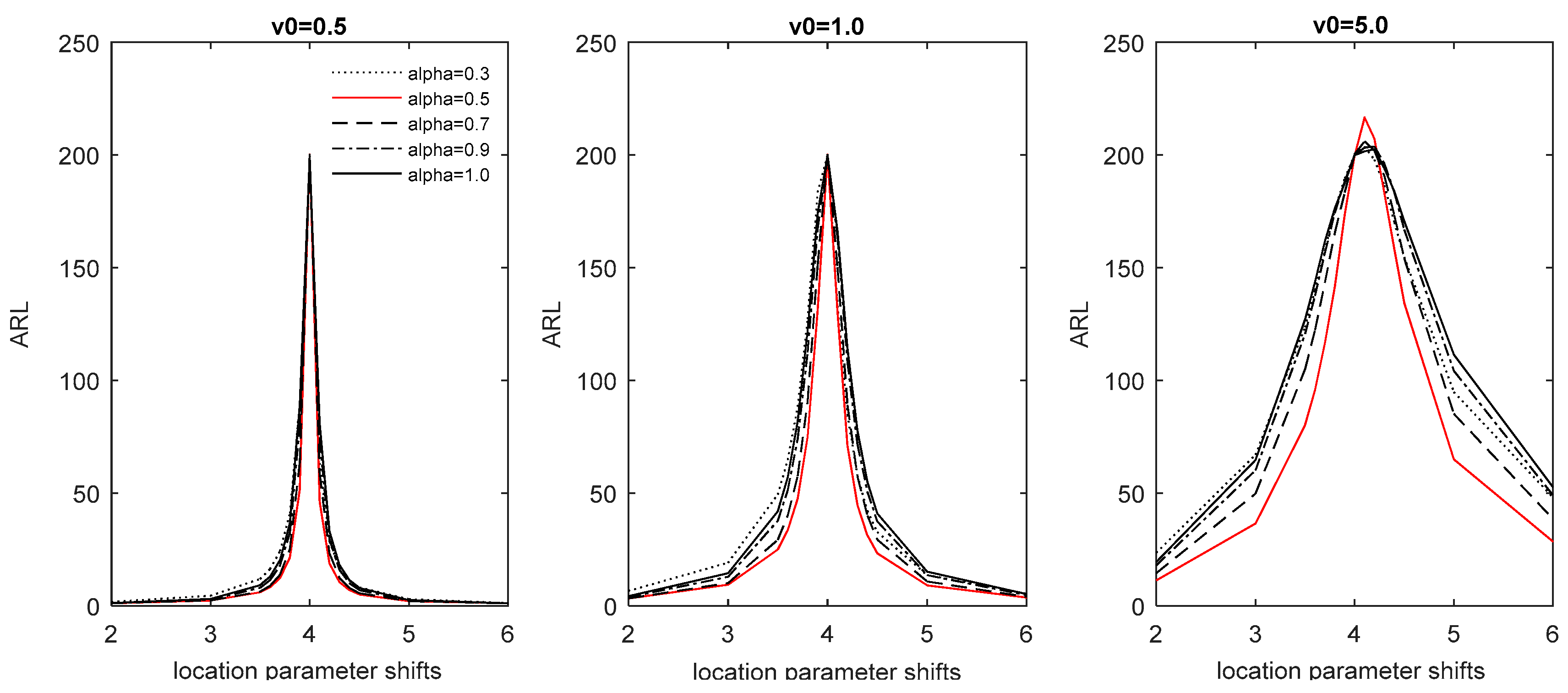
4.2.1. Location Parameter Shifts

Assume that the fixed dispersion parameter v = v 0 is known, and an assignable cause only displaces the location parameter μ . In other words, μ = δ μ 0 , where δ = {0.5, 0.75, 0.875, 0.9, 0.925, 0.95, 0.975, 1.025, 1.05, 1.075, 1.1, 1.125, 1.25, 1.5}, is considered in this study. According to the features of the COM-Poisson distribution, an upward (downward) shift in the location parameter results in the charts detecting an upward (downward) shift in the process mean. For each location parameter shift δ , under the design parameter q = {0.7, 0.9, 0.95} and the adjustment parameter α = {0.5, 0.7, 0.9, 1.0}, Table 3, Table 4 and Table 5 present the A R L s of the initial state CMP-GWMA and CMP-DGWMA charts with μ 0 = 4 for the fixed values of v 0 = 0.5 , v 0 = 1.0 and v 0 = 5.0 , respectively. For a clearer depiction, Figure 1 depicts the corresponding A R L s ’ curves of the CMP-DGWMA chart with q = 0.95 and α = 0.3, 0.5, 0.7, 0.9 and 1.0. In particular, when α = 1 and q = 1 λ , the CMP-GWMA and CMP-DGWMA charts are reduced, to the GEWMA chart by Saghir and Lin [15], and the CMP-DEWMA chart by Alevizakos and Koukouvinos [20], respectively.
The bold values in Table 3, Table 4 and Table 5 indicate the smallest A R L 1 values of the CMP-GWMA and CMP-DGWMA charts among the various location parameter shifts. The main findings from these tables are as follows:
(1).
For v 0 = 0.5 , the CMP-DGWMA chart is unbiased ( A R L 1 values are smaller than the A R L 0 value) when q 0.7 and α 0.5 . However, the CMP-GWMA chart is biased for a small downward shift ( δ = 0.975 ) when q 0.7 and α 0.5 . Moreover, the detection of upward shifts in CMP-GWMA and CMP-DGWMA charts in the location parameter is more sensitive than that for downward shifts. The simulation suggests that, among the proposed charts for monitoring small location shifts ( 0.95 δ 1.05 ) , a large value of q is recommended, and α near 0.5 is suitable for the CMP-DGWMA chart; however, α in the interval 0.5 α 0.7 is suitable for small upward shifts, while α in the interval 0.7 α 0.9 is suitable for small downward shifts for the CMP-GWMA chart.
(2).
For v 0 = 1.0 , the equally dispersed data follows a Poisson distribution. The CMP-DGWMA chart is the PDGWMA chart by Chiu and Lu [10]. When q 0.7 and α 0.5 , the CMP-GWMA and CMP-DGWMA charts are unbiased for upward shifts. Similar to the case of v 0 = 0.5 , the detection of upward shifts by these two charts is more sensitive than for downward shifts. Simulation results show that a CMP-DGWMA chart with large q and α near 0.5 is recommended for monitoring small location shifts. In addition, a CMP-GWMA chart with large q and α near 0.5 is suitable for small upward shifts; however, α in the interval 0.7 α 0.9 is suitable for small downward shifts.
(3).
For v 0 = 5.0 , the CMP-GWMA and CMP-DGWMA charts are almost unbiased for downward shifts, but a little biased for small upward shifts. In addition, unlike the cases of v 0 = 0.5 and v 0 = 1.0 , the CMP-GWMA and CMP-DGWMA charts detect downward shifts more sensitively than upward shifts. Simulation results show that a CMP-DGWMA chart with large q and α near 0.5, and a CMP-GWMA chart with large q and α near 0.7, are recommended for monitoring small downward shifts. Moreover, a CMP-DGWMA chart with q and α near 0.9 is suitable for small upward shifts.
(4).
To sum up, the larger the upward or downward shifts, the smaller the A R L 1 value for fixed parameter combinations of ( q , α ) . However, a larger value of v 0 results in a larger A R L 1 value. This result from the mean of the COM-Poisson distribution increases with an increase in the location parameter μ for a fixed value of v . At a minimum, a parameter combination of ( q , α ) can be obtained to clarify that CMP-DGWMA charts and CMP-GWMA charts perform substantially better than their respective prototypes (CMP-DEWMA charts and GEWMA charts). The CMP-DGWMA chart always performs better in detecting small location shifts than other charts.

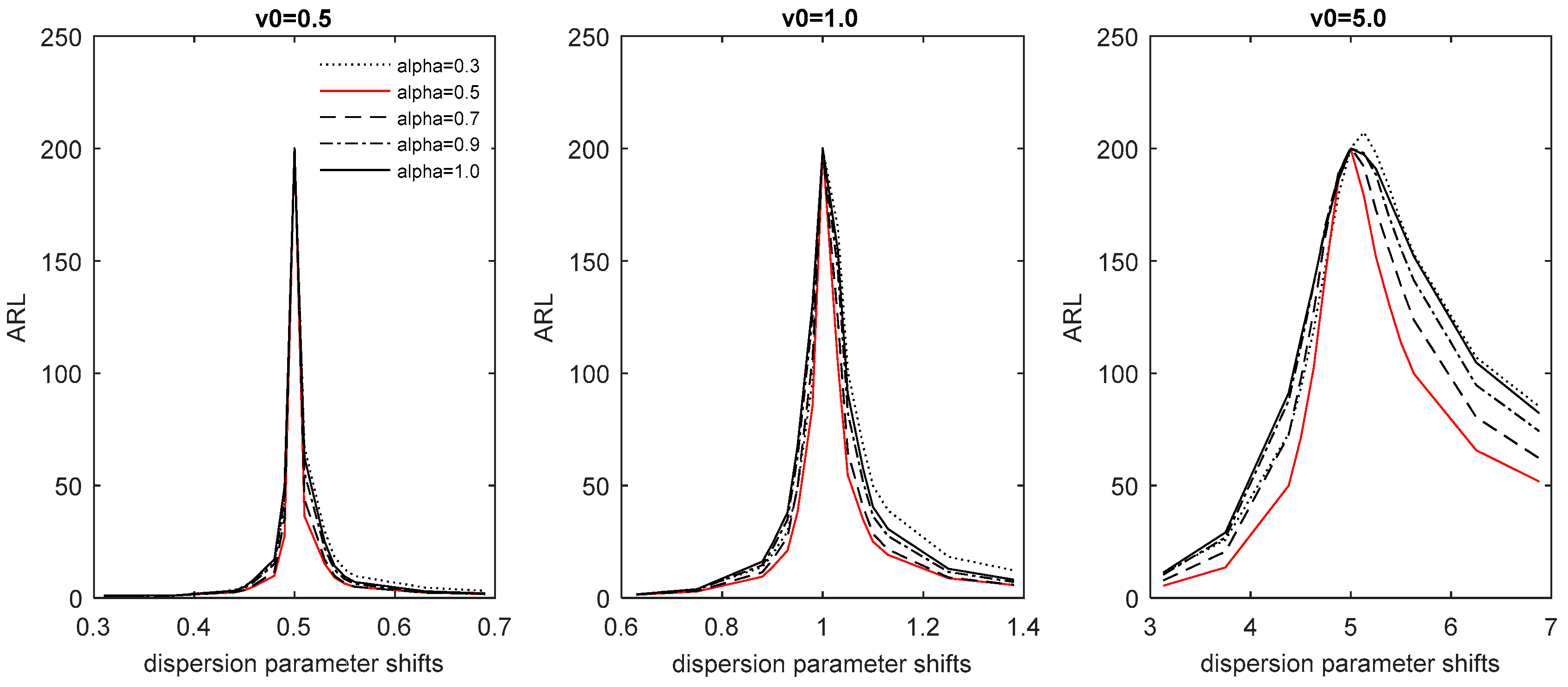
4.2.2. Dispersion Parameter Shifts

Assume that the fixed location parameter μ = μ 0 is known, and an assignable cause only displaces the dispersion parameter v , that is, v = τ v 0 , where τ = {0.625, 0.75, 0.875, 0.9, 0.925, 0.95, 0.975, 1.025, 1.05, 1.075, 1.1, 1.125, 1.25, 1.375} is considered in this study. According to the features of the COM-Poisson distribution, an upward (downward) shift in the dispersion parameter results in the charts detecting a downward (upward) shift in the process mean. For each dispersion parameter shift τ under the design parameter q = {0.7, 0.9, 0.95} and the adjustment parameter α = {0.5, 0.7, 0.9, 1.0}, Table 6, Table 7 and Table 8 present the A R L s of the initial state CMP-GWMA and CMP-DGWMA charts, with v 0 = 0.5 , v 0 = 1.0 and v 0 = 5.0 , respectively, for a fixed value of μ 0 = 4 . For a clearer perception, Figure 2 depicts the corresponding A R L s curves of the CMP-DGWMA chart with q = 0.95 and α = 0.3, 0.5, 0.7, 0.9 and 1.0. As with the previous case, the CMP-GWMA and CMP-DGWMA charts are respectively reduced to the GEWMA and CMP-DEWMA charts when α = 1 and q = 1 λ .
The bold values in Table 6, Table 7 and Table 8 indicate the smallest A L R 1 values of the CMP-GWMA and CMP-DGWMA charts among the various dispersion parameter shifts. The main findings from these tables are as follows:
(1).
For v 0 = 0.5 , the CMP-DGWMA chart is unbiased irrespective of downward or upward shifts, as long as q 0.7 and α 0.5 . The CMP-GWMA chart has the same features as the CMP-DGWMA chart, but is biased for small upward shifts ( τ = 1.025 ) when q 0.7 and α 0.5 . Moreover, the CMP-GWMA and CMP-DGWMA charts detect downward shifts in the dispersion parameter more sensitively than upward shifts. The simulation suggests that among the proposed charts for monitoring small dispersion shifts ( 0.95 τ 1.05 ) , a large value of q is recommended, and α near 0.5 is suitable for the CMP-DGWMA chart; α near 0.7 is suitable for small downward shifts. However, α in the interval 0.7 α 0.9 is suitable for small upward shifts for the CMP-GWMA chart.
(2).
For v 0 = 1.0 , the CMP-GWMA and CMP-DGWMA charts are unbiased for downward shifts when q 0.7 and α 0.5 . However, for small upward shifts, the CMP-DGWMA chart is biased when q 0.7 and α 1.0 ; the CMP-GWMA chart is biased when q 0.9 and α 1.0 , or when q 0.95 and α 0.5 . Similar to the previous case of v 0 = 0.5 , these two charts detect downward shifts more sensitively than upward shifts. Simulation results show that a CMP-DGWMA chart with large q and α near 0.5 is recommended for monitoring small dispersion shifts. In addition, a CMP-GWMA chart with large q and α near 0.5 is suitable for small downward shifts; however, α in the interval 0.7 α 0.9 is suitable for small upward shifts.
(3).
For v 0 = 5.0 , as in the cases of v 0 = 0.5 and v 0 = 1.0 , the CMP-GWMA and CMP-DGWMA charts are unbiased for downward shifts. For small upward shifts, the CMP-GWMA charts are always biased and the CMP-DGWMA charts are almost biased when q 0.9 and α 1.0 . Similar to the previous cases of v 0 = 0.5 and v 0 = 1.0 , these two charts detect downward shifts more sensitively than upward shifts. Simulation results show that a CMP-DGWMA chart with large q and α near 0.5, and a CMP-GWMA chart with large q and α in the interval 0.9 α 1.0 , are recommended to monitor small upward shifts. Moreover, for extremely small downward shifts, a CMP-DGWMA chart with q near 0.7 and α near 1.0 is recommended, and a CMP-GWMA chart with q near 0.7 and α near 0.5 is suggested.
(4).
To sum up, a smaller A R L 1 value corresponds to a larger downward dispersion shift for fixed parameter combinations of ( q , α ) . Similarly, for larger upward dispersion shifts, a smaller A R L 1 value always depends on specific parameter combinations of ( q , α ) , with a specific value of v 0 . Moreover, a larger value of v 0 results in a larger A R L 1 value. This result can be explained as follows. The mean of the COM-Poisson distribution decreases as the dispersion parameter v increases for a fixed value of μ . As previously mentioned, the CMP-DGWMA charts and CMP-GWMA charts are more sensitive than their prototype CMP-DEWMA charts and GEWMA charts, respectively, over the entire range of shifts in the dispersion parameter, except for the very small case of v 0 = 5.0 .

4.2.3. Both Location and Dispersion Parameter Shifts

Usually, one cannot identify which location parameters, dispersion parameters or both together are changed by an assignable cause in practice. Small location and dispersion parameter shifts are simultaneously investigated in this session. The COM-Poisson distribution with μ 0 = 4 corresponds to v 0 = 0.5 for over-dispersed data, v 0 = 1.0 for equally dispersed data, and v 0 = 5.0 for under-dispersed data; this is considered for the in-control process. In addition, the location parameter shifts from μ 0 to μ = δ μ 0 , and the dispersion parameter shifts from v 0 to v = τ v 0 , where δ , τ = {0.950, 0.975, 1.025, 1.050} is considered for the out-of-control process. Based on the results of the previous sessions, a large value of q is suitable for CMP-GWMA and CMP-DGWMA charts in detecting small location or dispersion parameter shifts. Hence, for two parameters’ simultaneous shifts under design parameter q = 0.95 and adjustment parameter α = {0.5, 0.7, 0.9, 1.0}, Table 9, Table 10 and Table 11 present the A R L s of the initial state CMP-GWMA and CMP-DGWMA charts, with v 0 = 0.5 , v 0 = 1.0 and v 0 = 5.0 , respectively, for a fixed value of μ 0 = 4 .
The bold values in Table 9, Table 10 and Table 11 indicate the smallest A R L 1 values of the CMP-GWMA and CMP-DGWMA charts among the various combinations of location and dispersion parameter shifts. The main findings from these tables are as follows:
(1).
For v 0 = 0.5 , the CMP-GWMA and CMP-DGWMA charts are unbiased for small shifts in both parameters when q = 0.95 and α 0.5 . For fixed values of q and α , both charts detect small upward location shifts, and downward dispersion shifts are more sensitive than other directional shifts. Based on the simulation, a large value of q is recommended for the proposed charts for monitoring small location and dispersion shifts simultaneously, and α near 0.5 is suitable for the CMP-DGWMA chart; however, α in the interval 0.7 α 0.9 is suitable for the CMP-GWMA chart.
(2).
For v 0 = 1.0 , the CMP-GWMA and CMP-DGWMA charts are almost unbiased, except for some cases of both upward location and dispersion shifts. Similar to the previous case of v 0 = 0.5 , these two charts perform well in detecting small upward location and downward dispersion shifts among any directional shifts. Based on the simulation results, a CMP-DGWMA chart with large q and α near 0.5 is recommended for monitoring small location and dispersion shifts simultaneously. In addition, a CMP-GWMA chart with large q and α near 0.5 is suitable for small downward dispersion shifts; however, α in the interval 0.7 α 0.9 is suitable for small upward dispersion shifts.
(3).
For v 0 = 5.0 , as in the previous case of v 0 = 1.0 , the CMP-GWMA and CMP-DGWMA charts are almost unbiased, in addition to there being some cases of both upward location and dispersion shifts. Similar to the cases of v 0 = 0.5 and v 0 = 1.0 , these two charts are not sensitive to detecting small upward location and downward dispersion shifts more than other directional shifts. Simulation results resemble the case of v 0 = 1.0 ; a large q and α near 0.5 is recommended for the CMP-DGWMA chart, for monitoring small location and dispersion shifts simultaneously. Similarly, a CMP-GWMA chart with large q and α near 0.5 is suitable for small downward dispersion shifts; however, α in the interval 0.7 α 0.9 is suitable for small upward dispersion shifts.
(4).
To sum up, a larger value of v 0 results in a larger A R L 1 value. Owing to the addition of design and adjustment parameters, the CMP-DGWMA and CMP-GWMA charts are more sensitive than their prototype CMP-DEWMA charts and GEWMA charts in detecting small location and dispersion shifts simultaneously.

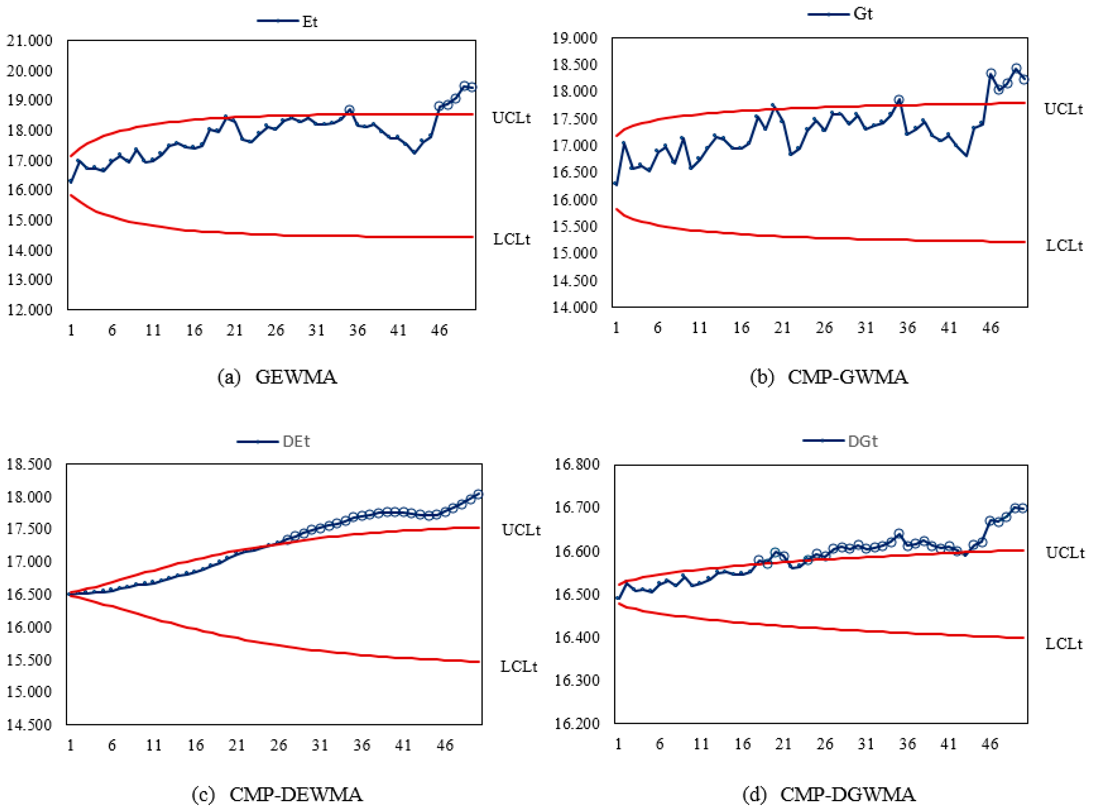
5. An Illustrative Example

This example uses a simulated dataset to illustrate the working of our proposed CMP-GWMA and CMP-DGWMA charts, and compare them with the existing GEWMA and CMP-EWMA charts when detecting small COM-Poisson process shifts at the initial stage. We assume that the monitored quality characteristic is over-dispersed and follows a COM-Poisson distribution, with μ 0 = 4 and v 0 = 0.5 . In addition, we assume that the underlying process location shifts from μ 0 to μ = δ μ 0 , and the dispersion shifts from v 0 to v = τ v 0 because of some assignable causes. For this purpose, when considering the process location, a small upward shift occurs for δ = 1.025 , and dispersion occurs with a small downward shift when τ = 0.975 . Table 12 shows that 50 individual samples ( X t ) are generated from a COM-Poisson distribution with μ = 4.1 and v = 0.4875 .
For a fair comparison, the in-control A R L values were set to 200 to investigate the detection ability of the existing and proposed charts. From Table 2, the charting parameter combinations ( q , α , L ) for the GEWMA, CMP-GWMA, CMP-DEWMA and CMP-DGWMA charts are (0.95, 1.0, 2.277), (0.95, 0.7, 2.400), (0.95, 1.0, 1.704) and (0.95, 0.5, 1.637), respectively. Moreover, their plotting statistics are represented as E t , G t , D E t and D G t , respectively. The corresponding time-varying upper and lower control limits of these charts are also listed in Table 12.
When an assignable cause results in small upward shifts ( δ = 1.025 ) in the process location and downward shifts ( τ = 0.975 ) in the process dispersion simultaneously, the GEWMA, CMP-GWMA, CMP-DEWMA and CMP-DGWMA charts trigger an out-of-control signal at the 35th, 35th, 26th and 18th samples, respectively. Corresponding to Table 9, the simulation results indicate that the GEWMA, CMP-GWMA and CMP-DEWMA charts respectively require 25.79, 23.39 and 23.29 samples on average to detect an out-of-control signal, whereas the CMP-DGWMA chart takes only 13.18 samples on average to identify an out-of-control signal. That is, the CMP-DGWMA chart detects small upward shifts in process location and downward shifts in process dispersion faster than its counterparts (the GEWMA, CMP-GWMA and CMP-DEWMA charts). Figure 3 displays the plotting statistics and corresponding control limits of the existing and proposed charts.

6. Conclusions

The COM-Poisson distribution is generalized to a Poisson distribution by location and dispersion parameters, which can be modeled for over-dispersed or under-dispersed attribute data, as well as for the geometric and Bernoulli distributions as special cases. The well-known GEWMA and CMP-DEWMA charts, based on COM-Poisson distribution, are used for monitoring the count of process defects or non-conformities. The CMP-DEWMA chart outperforms the GEWMA chart in detecting downward shifts of the mean value of the attribute process. To enhance the detection ability, this study integrates the features of a PGWMA chart to propose CMP-GWMA and CMP-DGWMA charts for the effective monitoring of small shifts in COM-Poisson processes. Note that the existing GEWMA and CMP-DEWMA charts are special cases of the CMP-GWMA and CMP-DGWMA charts, respectively.
A performance comparison between the proposed charts is maintained at the same value of in-control ARL, and then their out-of-control ARL values are compared for a process shift. The numerical simulations indicate that the CMP-DGWMA and CMP-GWMA charts are more sensitive than their respective prototypes (the CMP-DEWMA and GEWMA charts) in detecting small location and dispersion shifts, and both shifts together. Overall, the CMP-DGWMA chart always performs better in detecting small shifts than other charts. Finally, a simulated example is provided to illustrate the application of our proposed CMP-DGWMA chart, as well as that of its counterparts.

Funding

This research received no external funding.

Conflicts of Interest

The author declares no conflict of interest.

Appendix A

The novel statistic G t for the CMP-GWMA chart is defined as follows:
G t = j = 1 t ( q 1 ( j 1 ) α q 1 j α ) X t j + 1 + q 1 j α G 0 ,   0 q 1 < 1 ,   0 < α 1 .
We can represent Equation (A1) as follows:
G t = ( 1 q 1 1 α ) X t + ( q 1 1 α q 1 2 α ) X t 1 + + ( q 1 ( t 1 ) α q 1 t α ) X 1 + q 1 t α G 0 ,
where X t , t = 1 , 2 , 3 , is a COM-Poisson random variable that represents the number of non-conformities of a process at time t . For the in-control process, the mean and variance of the CMP-GWMA statistic G t are given as
E ( G t ) = ( 1 q 1 1 α ) E ( X t ) + ( q 1 1 α q 1 2 α ) E ( X t 1 ) + + ( q 1 ( t 1 ) α q 1 t α ) E ( X 1 ) + q 1 t α G 0 = E ( X t ) = μ 0 1 / v 0 v 0 1 2 v 0 ,
V a r ( G t ) = ( 1 q 1 1 α ) 2 V a r ( X t ) + ( q 1 1 α q 1 2 α ) 2 V a r ( X t 1 ) + + ( q 1 ( t 1 ) α q 1 t α ) 2 V a r ( X 1 ) = j = 1 t ( q 1 ( j 1 ) α q 1 j α ) 2 V a r ( X t ) = Q 1 t 1 v 0 μ 0 1 / v 0 .
Assuming that L denotes the width of the control limit, the upper and lower control limits and the central line of the CMP-GWMA chart are U C L t = E ( G t ) + L V a r ( G t ) , L C L t = M a x { 0 , E ( G t ) L V a r ( G t ) } and C L = E ( G t ) , respectively.
The CMP-DGWMA statistic D G t doubly smooths the sequence COM-Poisson random observations X t with the CMP-GWMA statistic G t from Equation (A1) as follows:
D G t = j = 1 t ( q 2 ( j 1 ) β q 2 j β ) G t j + 1 + q 2 t β G 0
where q 2 is the design parameter satisfying 0 q 2 < 1 , and β is the adjustment parameter satisfying 0 < β 1 . We can rewrite Equation (A5) as follows:
D G t = ( 1 q 2 1 β ) G t + ( q 2 1 β q 2 2 β ) G t 1 + + ( q 2 ( t 1 ) β q 2 t β ) G 1 + q 2 t β D G 0 = W 1 X t + W 2 X t 1 + + W t X 1 + ( 1 j = 1 t W j ) G 0 ,
where W t = ( 1 q 1 1 α ) ( q 2 ( t 1 ) β q 2 t β ) + ( q 1 1 α q 1 2 α ) ( q 2 ( t 2 ) β q 2 ( t 1 ) β ) + + ( q 1 ( t 1 ) α q 1 t α ) ( 1 q 2 1 β ) = j = 1 t ( q 1 ( j 1 ) α q 1 j α ) ( q 2 ( t j ) β q 2 ( t j + 1 ) β ) . For the in-control process, the mean and variance of the CMP-DGWMA statistic D G t are given as:
E ( D G t ) = E [ W 1 X t + W 2 X t 1 + + W t X 1 + ( 1 j = 1 t W j ) G 0 ] = E ( X t ) = μ 0 1 / v 0 v 0 1 2 v 0 ,
V a r ( D G t ) = V a r [ W 1 X t + W 2 X t 1 + + W t X 1 + ( 1 j = 1 t W j ) G 0 ] = j = 1 t W j 2 V a r ( X t ) = Q 2 t 1 v 0 μ 0 1 / v 0 .
Assuming that K denotes the width of the control limit, the upper and lower control limits and the central line of the CMP-GWMA chart are U C L t = E ( D G t ) + L V a r ( D G t ) , L C L t = M a x { 0 , E ( D G t ) L V a r ( D G t ) } and C L = E ( D G t ) , respectively.

References

  1. Brook, D.; Evans, D.A. An approach to the probability distribution of CUSUM run length. Biometrika 1972, 59, 539–549. [Google Scholar] [CrossRef]
  2. Lucas, J.M. Counted data CUSUM’s. Technometrics 1985, 27, 129–144. [Google Scholar] [CrossRef]
  3. White, C.H.; Keats, J.B. ARLs and higher-order run-length moments for the Poisson CUSUM. J. Qual. Technol. 1996, 28, 363–369. [Google Scholar] [CrossRef]
  4. White, C.H.; Keats, J.B.; Stanley, J. Poisson CUSUM vs. c-chart for detect data. Qual. Eng. 1997, 9, 673–679. [Google Scholar] [CrossRef]
  5. Gan, F.F. Monitoring poisson observations using modified exponentially weighted moving average control charts. Commun. Stat. Simul. Comput. 1990, 19, 103–124. [Google Scholar] [CrossRef]
  6. Borror, C.M.; Champ, C.W.; Rigdon, S.E. Poisson EWMA control charts. J. Qual. Technol. 1998, 30, 352–361. [Google Scholar] [CrossRef]
  7. Zhang, L.; Govindaraju, K.; Lai, C.D.; Bebbington, M.S. Poisson DEWMA control chart. Commun. Stat. Simul. Comput. 2003, 32, 1265–1283. [Google Scholar] [CrossRef]
  8. Sheu, S.H.; Chiu, W.C. Poisson GWMA control chart. Commun. Stat. Simul. Comput. 2007, 36, 1099–1114. [Google Scholar] [CrossRef]
  9. Chiu, W.C.; Sheu, S.H. Fast initial response features for Poisson GWMA control charts. Commun. Stat. Simul. Comput. 2008, 37, 1422–1439. [Google Scholar] [CrossRef]
  10. Chiu, W.C.; Lu, S.L. On the steady-state performance of the Poisson Double GWMA control chart. Qual. Technol. Quant. Manag. 2015, 12, 195–208. [Google Scholar] [CrossRef]
  11. Conway, R.W.; Maxwell, W.L. A queuing model with state dependent service rates. J. Ind. Eng. 1962, 12, 132–136. [Google Scholar]
  12. Sellers, K.F. A generalized statistical control chart for over- or under- dispersed data. Qual. Reliab. Eng. Int. 2012, 28, 59–65. [Google Scholar] [CrossRef]
  13. Saghir, A.; Lin, Z.; Abbasi, S.A.; Ahmad, S. The use of probability control limits of the COM-poisson charts and their applications. Qual. Reliab. Eng. Int. 2013, 29, 759–770. [Google Scholar] [CrossRef]
  14. Saghir, A.; Lin, Z. Cumulative sum charts for monitoring the COM-Poisson processes. Comput. Ind. Eng. 2014, 68, 65–77. [Google Scholar] [CrossRef]
  15. Saghir, A.; Lin, Z. A flexible and generalized exponentially weighted moving average control chart for count data. Qual. Reliab. Eng. Int. 2014, 30, 1427–1443. [Google Scholar] [CrossRef]
  16. Aslam, M.; Ahmad, L.; Jun, C.H.; Arif, O.H. A control chart for COM-Poisson distribution using multiple dependent state sampling. Qual. Reliab. Eng. Int. 2016, 32, 2803–2812. [Google Scholar] [CrossRef]
  17. Aslam, M.; Azam, M.; Jun, C.H. A control chart for COM-Poisson distribution using resampling and exponentially weighted moving average. Qual. Reliab. Eng. Int. 2016, 32, 727–735. [Google Scholar] [CrossRef]
  18. Aslam, M.; Saghir, A.; Ahmad, L.; Jun, C.H.; Hussain, J. A control chart for COM-Poisson distribution using a modified EWMA statistic. J. Stat. Comput. Simul. 2017, 87, 3491–3502. [Google Scholar] [CrossRef]
  19. Aslam, M.; Khan, N.; Jun, C.H. A hybrid exponentially weighted moving average chart for COM-Poisson distribution. Trans. Inst. Meas. Control. 2018, 40, 456–461. [Google Scholar] [CrossRef]
  20. Alevizakos, V.; Koukouvinos, C. A double exponentially weighted moving average control chart for monitoring COM-Poisson attributes. Qual. Reliab. Eng. Int. 2019, 35, 2130–2151. [Google Scholar] [CrossRef]
  21. Shmueli, G.; Minka, T.P.; Kadane, J.B.; Borle, S.; Boatwright, P. A useful distribution for fitting discrete data: Revival of the Conway–Maxwell–Poisson distribution. Appl. Stat. 2005, 54, 127–142. [Google Scholar] [CrossRef]
  22. Montgomery, D.C. Introduction to Statistical Quality Control, 6th ed.; John Wiley & Sons, Inc.: New York, NY, USA, 2009. [Google Scholar]
  23. Lu, S.L. Non parametric double generally weighted moving average sign charts based on process proportion. Commun. Stat. Theory Methods 2018, 47, 2684–2700. [Google Scholar] [CrossRef]
Figure 1. ARL curves of the CMP-DGWMA chart with q = 0.95 and α = 0.3, 0.5, 0.7, 0.9 and 1.0, for various location parameter shifts at μ 0 = 4
Symmetry 12 01014 g001
Figure 2. Curves of the CMP-DGWMA chart with q = 0.95 and α =0.3, 0.5, 0.7, 0.9 and 1.0, for various dispersion parameter shifts at v 0 =0.5, 1.0 and 5.0, and fixed value of μ 0 = 4
Symmetry 12 01014 g002
Figure 3. The statistics and control limits of the GEWMA, CMP-GWMA, -DEWMA and -DGWMA charts, at process location shift μ = 4.1 and dispersion v = 0.4875 .
Symmetry 12 01014 g003
Table 1. Three well known distributions from the Conway–Maxwell–Poisson (COM-Poisson) distribution.
Condition z ( μ , v ) P ( x ; μ , v ) Distribution
μ < 1 , v = 0 j = 0 μ j = 1 1 μ μ x ( 1 μ ) Geometric
v = 1 j = 0 μ j j ! = e μ e μ μ x x ! Poisson
v 1 + μ μ 1 + μ Bernoulli
Table 2. L ( K ) values for the Conway–Maxwell–Poisson GWMA (CMP-GWMA) and CMP-Double GWMA (CMP-DGWMA) charts, for μ 0 = 4 and A R L 0 200 .
CMP-GWMA α
v 0 q 0.10.20.30.40.50.60.70.80.91.0
0.50.52.8882.8772.8682.8592.8522.8432.8342.8282.8222.814
0.62.8862.8722.8572.8452.8312.8202.8102.7992.7892.781
0.72.8842.8672.8462.8232.8042.7872.7672.7522.7382.727
0.82.8832.8622.8302.7962.7652.7332.7052.6792.6592.646
0.92.8822.8542.8122.7572.6912.6242.5652.5232.4932.477
0.952.8812.8512.8012.7302.6232.5052.4002.3312.2922.277
1.00.53.0002.9872.9672.9482.9332.9132.8972.8872.8732.863
0.62.9992.9792.9472.9212.8942.8722.8512.8342.8182.808
0.72.9982.9692.9252.8842.8482.8182.7942.7742.7572.745
0.82.9962.9582.8962.8342.7862.7502.7172.6862.6622.648
0.92.9942.9462.8622.7762.6992.6272.5652.5202.4992.478
0.952.9932.9392.8422.7382.6262.5012.4002.3282.2862.272
5.00.52.2012.2922.3842.4742.5522.6212.6822.7302.7682.800
0.62.2112.3122.4242.5302.6242.7002.7572.8002.8282.850
0.72.2202.3342.4642.5882.6872.7582.8042.8392.8572.866
0.82.2292.3572.5042.6372.7272.7742.7972.7982.7942.786
0.92.2362.3782.5412.6702.7182.7112.6802.6412.6032.571
0.952.2402.3882.5582.6732.6752.5982.5072.4352.3722.329
CMP-DGWMA α
0.50.52.8742.8392.8022.7702.7412.7182.6992.6892.6812.678
0.62.8692.8192.7622.7062.6572.6212.5992.5882.5832.585
0.72.8642.7972.7042.6012.5222.4742.4532.4462.4492.462
0.82.8592.7732.6142.4202.2872.2302.2192.2312.2542.286
0.92.8542.7412.4712.1201.9001.8251.8261.8641.9241.993
0.952.8522.7242.3761.9111.6371.5171.5091.5521.6251.704
1.00.52.9832.9122.8452.7942.7612.7342.7102.6942.6862.682
0.62.9742.8752.7822.7182.6632.6242.6012.5882.5842.583
0.72.9652.8352.7112.6012.5202.4782.4512.4492.4562.468
0.82.9552.7942.6152.4192.2842.2252.2162.2282.2552.287
0.92.9452.7522.4732.1191.9071.8191.8211.8661.9271.998
0.952.9402.7302.3731.9181.6291.5061.5001.5421.6211.704
5.00.52.2892.4882.6602.7622.8152.8362.8442.8422.8312.822
0.62.3102.5412.7092.7702.7722.7542.7332.7122.6942.682
0.72.3292.5882.7162.6992.6412.5802.5352.5132.5102.519
0.82.3492.6232.6702.5232.3872.2952.2422.2452.2872.332
0.92.3702.6442.5512.2141.9811.8501.8531.9061.9702.045
0.952.3792.6482.4632.0131.7401.5891.5581.6251.6951.790
Table 3. A R L s of CMP-GWMA and CMP-DGWMA charts for μ 0 = 4 , fixed value of v 0 = 0.5 and A R L 0 200 .
δ
q α L ( K ) 0.50.750.8750.90.9250.950.97511.0251.051.0751.11.1251.251.5
0.70.52.8042.818.1828.4443.3774.83149.96270.60199.7592.2546.8527.8218.2012.844.031.42
2.5221.964.8113.5419.0529.5053.58123.91200.1284.9837.4520.9613.529.523.191.29
0.72.7672.506.7724.4338.7569.05139.55245.44199.9097.5748.4627.6417.5712.163.801.40
2.4531.904.5413.2419.1230.6958.82134.03200.2296.1841.9022.7714.269.853.191.29
0.92.7382.266.2425.1641.0773.95143.97236.89199.82104.1052.0329.2518.1812.303.641.35
2.4491.914.6614.4821.5936.4070.80150.38200.27104.9947.8125.3815.6610.583.301.29
1.02.7272.226.1926.4343.4678.55149.32235.18199.90106.5154.1230.4118.7412.593.641.35
2.4621.934.7715.5223.6040.4678.45160.05199.52108.1650.5826.9516.4511.013.381.30
0.90.52.6912.406.3318.0525.2238.4468.02148.12199.7179.1637.8022.3514.9410.693.611.35
1.9001.363.007.8410.8816.5829.4670.71200.0161.6625.0013.798.926.352.371.16
0.72.5652.145.1014.2119.9930.8155.71128.51199.9883.5237.3321.1213.759.763.331.34
1.8261.252.908.2611.6718.2433.1881.51200.0773.5529.5415.9210.036.952.371.13
0.92.4931.924.6513.3619.1030.2557.29132.01199.6791.6840.1622.0313.919.673.191.29
1.9241.373.409.9914.1722.1440.3498.71200.0087.2335.5619.3312.198.432.711.17
1.02.4771.914.6113.5019.5531.6160.91137.74200.1496.6142.2422.9514.349.893.211.29
1.9931.393.6910.8415.3924.1044.70107.31200.2892.7338.5320.7613.109.082.881.17
0.950.52.6232.305.8616.1722.3633.7158.22126.01199.7274.9435.2520.8113.9810.063.491.35
1.6371.162.386.038.2012.2721.4251.36200.2546.2218.6910.536.995.082.041.10
0.72.4001.914.4512.0416.7025.4344.67103.60200.0676.7133.0618.6712.208.673.051.28
1.5091.162.366.358.8913.8025.1763.47200.4058.7623.1312.377.935.612.081.10
0.92.2921.694.0211.1715.7624.3844.36105.11200.2883.7935.2319.3412.308.602.901.24
1.6251.162.698.0411.4017.8132.4179.59199.9173.2429.4016.0010.106.992.311.11
1.02.2771.704.0311.3316.0925.1046.31110.02200.1188.5237.2220.1812.738.872.941.24
1.7041.253.059.1812.9920.1836.4888.74200.0980.9133.0118.1111.467.962.551.14
Upper: ARLs of CMP-GWMA chart; Lower: ARLs of CMP-DGWMA chart.
Table 4. A R L s of CMP-GWMA and CMP-DGWMA charts for μ 0 = 4 , fixed value of v 0 = 1.0 and A R L 0 200
δ
q α L ( K ) 0.50.750.8750.90.9250.950.97511.0251.051.0751.11.1251.251.5
0.70.52.84815.4175.81342.20424.61435.23365.12276.78200.03145.74108.8983.4965.1352.3822.328.11
2.5207.0722.3765.4188.41124.40171.70210.91200.39153.92109.5877.7057.0043.7317.166.30
0.72.79411.6662.35264.76322.98345.48320.78261.46199.76150.52114.5787.3767.9353.7921.797.60
2.4516.4022.1771.3297.05134.13176.54207.59200.25161.95120.8788.4865.2849.0918.136.14
0.92.75710.7865.64246.10290.29313.27296.54250.74200.00154.59120.2692.8272.5257.4522.817.59
2.4566.7225.9488.62118.45156.01194.24214.74199.99165.66128.5097.7773.6655.9120.236.58
1.02.74510.8070.49248.02287.54305.61291.49249.71200.01157.27122.8995.7975.2159.7323.607.67
2.4686.9628.8599.92131.70168.28202.87217.04199.81166.00129.97100.1776.3858.4421.266.79
0.90.52.6999.9031.4989.97120.02163.82217.24244.06199.98140.5997.6570.8953.5442.2018.157.00
1.9074.0512.2034.2245.8865.49100.49159.13199.97147.8689.9658.4040.9630.2311.324.25
0.72.5657.4623.6068.9193.40131.33180.56216.58200.00150.39106.3675.7055.9542.9817.186.40
1.8214.1413.2338.5452.2775.45113.65168.30200.21161.00106.3870.5349.9836.8113.304.63
0.92.4996.7022.3470.3096.03134.12179.43210.98199.77159.15116.7684.4361.6646.7917.636.11
1.9274.7415.6946.1763.2990.37131.69179.27200.15167.71118.1881.9958.4743.3515.855.40
1.02.4786.5922.8574.57101.83139.86182.02210.83200.10161.01120.6288.7465.5749.4118.276.19
1.9985.1316.9851.0970.3199.84141.13185.68200.21169.67123.3286.9062.6446.5616.945.79
0.950.52.6268.9227.2373.5896.76132.46181.58224.14200.23140.1494.9067.5150.4939.6516.986.64
1.6293.309.3324.9933.5947.6375.23131.00200.21130.0771.1044.7231.2523.309.113.68
0.72.4006.3519.2453.0571.2199.33142.51193.54199.99150.95101.4569.7850.4138.4015.025.58
1.5003.3110.0729.3040.1257.6690.87151.04200.25150.1589.1657.4239.9729.3910.813.97
0.92.2865.7317.9351.6670.4499.52141.99189.98199.68159.30112.5877.9656.1742.1615.745.57
1.6213.8312.8637.7651.2974.14112.42167.25200.17163.51108.1071.5750.6637.4513.634.73
1.02.2725.6718.1753.8373.52104.19146.37190.77199.67162.41117.7282.6259.5844.5316.375.69
1.7044.2914.4441.9157.0481.93122.34174.00199.96165.99114.3477.4855.0440.9115.185.23
Upper: ARLs of CMP-GWMA chart; Lower: ARLs of CMP-DGWMA chart.
Table 5. A R L s of CMP-GWMA and CMP-DGWMA charts for μ 0 = 4 , fixed value of v 0 = 5.0 and A R L 0 200
δ
q α L ( K ) 0.50.750.8750.90.9250.950.97511.0251.051.0751.11.1251.251.5
0.70.52.68745.89137.82192.70199.53203.33203.61202.55200.02195.04187.64179.76170.06161.28120.7571.12
2.64129.2588.67150.91164.06176.91188.38196.52200.15202.38200.53195.47187.48179.21128.3968.14
0.72.80446.85137.63187.60194.16198.67200.37200.22199.60196.84192.09186.92179.66172.62135.7783.27
2.53530.5794.95154.40165.73177.05187.74195.42199.82202.38201.74199.55193.76188.03145.8581.07
0.92.85749.54138.83184.31190.41195.16198.45199.47199.85198.62195.72192.11186.73180.48148.2994.14
2.51033.63104.38161.33172.25181.63189.74195.82200.13202.68202.62201.71197.70192.21157.7194.35
1.02.86650.68138.14183.22189.45194.18197.50199.37200.06199.58197.18194.31189.77184.69153.7299.80
2.51938.59113.70167.21176.54184.66191.90196.27199.83201.98201.08199.62195.62190.93159.4797.62
0.90.52.71834.0896.90159.43172.10184.40193.06199.30200.52197.82193.12185.80175.86164.74115.6563.34
1.98117.0454.19109.11126.82146.30166.70184.93199.63205.27202.34193.14177.87161.4293.5443.42
0.72.68029.9490.21152.97166.18178.49189.04196.37200.07201.28199.02193.19184.52175.40124.9466.57
1.85320.2765.31127.99145.40161.65177.96192.87200.82204.57203.52195.71184.31170.32107.8451.29
0.92.60330.3193.70154.25165.84177.93188.36195.17199.91201.55200.26197.23191.03184.46138.9575.89
1.97024.5478.46141.19155.62169.69182.38192.87199.93201.60199.49195.80186.72177.21121.8960.58
1.02.57131.4597.15156.67167.64178.47188.82195.64199.79202.05201.30199.32193.71187.92146.6181.99
2.04526.3884.11147.15160.50173.65185.02194.28199.83202.32199.67196.54188.79180.31128.6365.92
0.950.52.67530.7087.34149.29163.23178.19188.45196.82200.24199.05194.22185.64174.29161.58110.0658.91
1.74011.2736.4780.3095.80116.57141.63173.47199.81216.62206.96182.78157.98134.3265.0028.44
0.72.50725.4776.37137.94153.31168.28182.56193.16200.13199.89198.72192.77182.39170.87114.5558.21
1.55814.5449.78105.02122.32143.39165.51183.40200.35206.04201.93190.52173.16154.1285.1338.53
0.92.37224.8278.17140.06154.93169.08182.06192.93199.48201.72201.65197.49188.80180.92126.2664.35
1.69517.9660.09120.64137.55156.68174.47188.45199.99203.24203.66196.12183.28166.84104.2049.04
1.02.32925.5481.30143.71157.98170.91183.01193.31200.15203.09203.12199.97192.42185.43133.5469.24
1.79019.4264.69127.03143.74161.71176.27187.57199.91201.60202.51193.87183.85170.56111.4352.53
Upper: ARLs of CMP-GWMA chart; Lower: ARLs of CMP-DGWMA chart.
Table 6. A R L s of CMP-GWMA and CMP-DGWMA charts for v 0 = 0.5 , fixed value of μ 0 = 4 and A R L 0 200
τ
q α L ( K ) 0.6250.7500.8750.9000.9250.9500.9751.01.0251.0501.0751.1001.1251.2501.375
0.70.52.8041.001.244.777.4512.8425.2362.55199.75253.91105.2652.4332.3422.668.625.48
2.5221.001.173.815.799.7819.5553.54200.1292.0437.2321.3014.4010.774.863.33
0.72.7671.001.234.517.0612.2725.0165.67199.90231.9798.4847.2927.7818.986.994.50
2.4531.001.173.855.9210.2121.2561.22200.22101.8439.7821.4814.0710.334.543.10
0.92.7381.001.204.356.9412.4126.2869.89199.82226.31106.0051.3729.2319.176.404.07
2.4491.001.174.016.2311.0023.4968.65200.27120.3248.3824.7315.4911.014.643.15
1.02.7271.001.204.367.0112.7227.3372.32199.90227.69111.7954.8331.0920.076.333.97
2.4621.001.174.116.4311.4524.7671.95199.52131.4554.1827.3616.7611.684.743.21
0.90.52.6911.001.204.266.5110.8320.7051.85199.71112.9448.6728.5119.5414.716.534.40
1.9001.001.102.794.066.6012.9637.20200.0150.0020.4611.988.266.293.002.13
0.72.5651.001.203.955.9710.0119.6752.84199.9895.6438.8422.3415.1711.395.173.55
1.8261.001.082.864.307.3115.0144.46200.0757.2322.6412.868.666.462.861.96
0.92.4931.001.173.835.8610.0120.5058.05199.6799.8838.9721.4314.2210.514.683.21
1.9241.001.103.325.138.8818.3353.67200.0070.1727.5415.5610.437.763.342.26
1.02.4771.001.173.875.9410.2421.3961.71200.14105.8041.2222.0314.3610.524.623.16
1.9931.001.103.555.539.5419.6457.58200.2877.6130.0916.9111.338.453.632.40
0.950.52.6231.001.204.116.2210.1819.3648.65199.7295.7241.9125.0717.4213.236.034.09
1.6371.001.062.393.365.259.8827.62200.2536.2815.189.036.344.862.361.69
0.72.4001.001.173.615.388.9317.4947.64200.0675.5231.4518.5412.799.654.493.14
1.5091.001.062.473.575.8611.7135.13200.4043.7517.139.776.644.982.311.66
0.92.2921.001.143.465.258.9518.1751.96200.2876.1530.3917.4711.818.844.022.79
1.6251.001.072.834.297.3515.1344.66199.9155.5222.0012.518.396.182.621.77
1.02.2771.001.143.535.389.2518.9855.03200.1180.1631.4217.8411.968.914.012.79
1.7041.001.083.154.878.3917.1449.66200.0962.6024.9514.229.567.072.971.99
Upper: ARLs of CMP-GWMA chart; Lower: ARLs of CMP-DGWMA chart.
Table 7. A R L s of CMP-GWMA and CMP-DGWMA charts for v 0 = 1.0 , fixed value of μ 0 = 4 and A R L 0 200
τ
q α L ( K ) 0.6250.7500.8750.9000.9250.9500.9751.01.0251.0501.0751.1001.1251.2501.375
0.70.52.8482.005.3221.0630.0844.6769.91115.62200.03346.37516.65555.10429.30299.8879.2240.78
2.5201.884.5117.4525.4439.3666.31120.84200.39209.72143.4794.3166.1249.8520.9613.33
0.72.7941.965.0820.8830.3145.8073.17120.89199.76317.21411.94414.08331.60245.1367.0132.34
2.4511.744.3818.6027.7043.9074.99130.40200.25209.05156.06105.8373.5354.4020.6212.54
0.92.7571.965.0621.8032.0948.7277.45125.93200.00298.23372.42372.57313.71244.8574.3534.71
2.4561.804.6820.6331.2049.4583.36136.50199.99222.82182.25133.2295.1070.3524.4013.81
1.02.7451.955.0922.4533.2450.5080.01127.99200.01295.21365.09369.72320.24257.1682.4938.30
2.4681.824.8021.4932.4851.4784.99137.36199.81229.88197.70149.80108.8781.3927.6515.06
0.90.52.6991.944.8117.8125.2237.4360.43107.80199.98256.51191.32129.6992.4370.4630.6219.67
1.9071.493.2111.7317.3427.4549.75105.96199.97134.3974.3647.3633.6525.6611.367.41
0.72.5651.894.5617.3725.1538.6364.86117.80200.00219.33152.0299.9869.7252.5822.3014.25
1.8211.523.4714.0821.0933.9160.88123.26200.21146.9184.1753.2837.3828.3912.007.63
0.92.4991.744.3418.0326.6341.8371.40126.47199.77214.47155.84104.1572.1653.4220.8512.92
1.9271.593.9916.7725.0240.1570.74133.44200.15164.30101.7764.8245.0833.9914.228.94
1.02.4781.754.4118.6827.8244.1075.08129.67200.10214.53163.04111.5377.6057.1021.2712.87
1.9981.634.2517.8926.6642.7975.17136.98200.21174.14113.1372.6850.1937.5215.439.70
0.950.52.6261.924.6416.8123.6935.3657.62105.82200.23223.88152.33102.7674.7457.9826.3417.27
1.6291.452.879.4013.5921.1238.0585.37200.21104.5154.6334.8524.9519.158.735.75
0.72.4001.714.0215.3322.3134.7959.83114.70199.99181.05112.7273.9752.9340.5218.0511.78
1.5001.463.0511.4116.9226.9949.31106.81200.25124.2664.7040.7528.5721.529.115.82
0.92.2861.714.0616.3324.2138.2766.99125.53199.68177.67113.4973.1351.2538.7516.5310.56
1.6211.533.5714.5821.8034.8462.36125.70200.17145.8582.2151.9236.3327.4611.537.15
1.02.2721.724.1417.1225.4340.4570.74130.39199.67181.37118.8376.5653.3840.0416.6710.55
1.7041.583.9016.1823.9838.0867.42130.94199.96154.6390.9957.6540.4430.6312.958.10
Upper: ARLs of CMP-GWMA chart; Lower: ARLs of CMP-DGWMA chart.
Table 8. A R L s of CMP-GWMA and CMP-DGWMA charts for v 0 = 5.0 , fixed value of μ 0 = 4 and A R L 0 200
τ
q α L ( K ) 0.6250.7500.8750.9000.9250.9500.9751.01.0251.0501.0751.1001.1251.2501.375
0.70.52.68714.7133.4585.00102.07123.15147.11173.92200.02224.94248.45282.74267.53290.91280.52245.97
2.64114.3234.8094.90115.46138.32164.04185.51200.15211.27212.79209.53204.87195.61150.74123.34
0.72.80415.4936.2092.30109.95129.91152.57176.52199.60221.05241.47270.94257.47279.52280.93258.45
2.53515.5838.82103.21123.08144.66165.59186.15199.82208.83212.56212.84210.77205.68170.25145.44
0.92.85715.8538.6997.25115.36135.20156.64178.68199.85219.11236.77264.13251.83272.23282.85267.37
2.51016.7041.58107.06126.58146.33165.83185.21200.13211.87220.07222.60223.68221.84199.71177.12
1.02.86616.3540.25100.17118.14137.53158.33180.05200.06218.51235.25261.97249.36270.04282.11269.84
2.51917.5043.06107.82126.93146.64165.62184.42199.83212.91222.17226.56230.21230.96215.00195.51
0.90.52.71814.3732.8186.17105.51128.30153.68179.00200.52217.38223.05219.18223.90209.48160.69130.77
1.9818.7022.1873.4797.14125.88158.90186.45199.63196.35181.75164.69148.28133.5388.9969.82
0.72.68014.0834.0292.55113.31136.29161.65183.90200.07211.69214.42207.42212.02198.89152.76124.39
1.85310.8028.4689.26112.06138.71166.95188.23200.82202.17195.10181.63167.59152.57104.3582.47
0.92.60314.9737.1799.65119.51141.33164.13184.74199.91209.52213.24210.46212.64204.71166.69140.17
1.97013.0433.7498.46119.78144.02167.67187.19199.93203.92200.90195.05185.92175.95130.47105.42
1.02.57115.5738.81102.95122.78144.17165.30185.70199.79209.69214.52213.44215.41209.41175.85151.18
2.04513.8435.59101.52122.71145.93168.03186.42199.83205.92206.34201.72195.94186.80144.71119.15
0.950.52.67513.4031.0283.38102.98126.53153.08178.51200.24213.37215.67201.90210.87189.57140.17113.07
1.7405.4613.5249.8970.97102.36145.20187.53199.81178.75151.68130.92113.5899.7965.6651.79
0.72.50712.7230.9388.31109.77134.71160.42183.30200.13207.10203.16184.21194.94171.66122.4498.01
1.5587.7820.6472.5197.19127.64162.38189.63200.35192.02172.79154.91138.92123.6080.4562.09
0.92.37213.4833.7496.59118.32141.78165.52185.93199.48205.75202.40187.61196.10177.17129.94104.98
1.69510.4026.9387.76111.77139.46166.56189.02199.99198.03188.26169.79155.26141.2894.7174.17
1.02.32914.2335.87100.37122.36144.87168.24187.75200.15205.51204.41191.95199.70182.33139.02113.32
1.79011.2829.1791.21115.22140.05165.09186.64199.91197.33190.95177.58165.33151.91104.6982.16
Upper: ARLs of CMP-GWMA chart; Lower: ARLs of CMP-DGWMA chart.
Table 9. A R L s of CMP-GWMA and CMP-DGWMA charts for μ 0 = 4 , v 0 = 0.5 and A R L 0 200
q = 0.95 , α = 0.5 q = 0.95 , α = 0.7
τ \ δ 0.9500.9751.0001.0251.0500.9500.9751.0001.0251.050
0.95080.7034.4519.3612.648.9084.6232.8817.4911.067.74
53.8418.579.886.414.6169.2923.3511.717.265.05
0.975162.86128.4148.6525.5515.98140.39136.0847.6423.3914.09
79.19104.9927.6213.188.0398.37127.8435.1315.949.27
1.00058.22126.01199.7274.9435.2544.67103.60200.0676.7133.06
21.4251.36200.2546.2218.6925.1763.47200.4058.7623.13
1.02530.5649.1495.72216.37128.7322.8437.3375.52192.99134.78
11.0317.8936.28124.4896.3112.2320.5543.75144.15117.88
1.05019.8527.6941.9173.67162.3314.6720.5731.4556.54132.22
7.239.9715.1826.9467.387.7310.9217.1331.7681.87
q = 0.95 , α = 0.9 q = 0.95 , α = 1.0
0.95092.8535.1518.1711.167.6897.3837.2418.9811.607.92
85.7029.8015.139.246.2692.8833.4017.1410.527.13
0.975142.03145.5351.9624.5614.40146.31149.9155.0325.7915.01
118.42142.5244.6620.6111.86127.72148.9149.6623.2913.52
1.00044.36105.11200.2883.7935.2346.31110.02200.1188.5237.22
32.4179.59199.9173.2429.4036.4888.74200.0980.9133.01
1.02521.7536.4276.15190.60144.8822.2938.0080.16192.49149.91
15.7726.5455.52161.72134.1617.9229.9162.60171.77142.40
1.05013.7019.4630.3956.22134.2613.9119.9031.4259.32140.27
9.8314.0122.0040.59101.5311.2115.9424.9545.60112.18
Upper: ARLs of CMP-GWMA chart; Lower: ARLs of CMP-DGWMA chart.
Table 10. A R L s of CMP-GWMA and CMP-DGWMA charts for μ 0 = 4 , v 0 = 1.0 and A R L 0 200
q = 0.95 , α = 0.5 q = 0.95 , α = 0.7
τ \ δ 0.9500.9751.0001.0251.0500.9500.9751.0001.0251.050
0.950122.9882.3057.6242.8133.57133.1787.8159.8342.7032.42
113.0960.8938.0526.2419.56134.7777.9349.3133.8824.72
0.975206.28157.97105.8273.0953.07192.22166.93114.7076.5653.89
163.13158.9985.3750.9433.87173.15175.66106.8165.5443.47
1.000181.58224.14200.23140.1494.90142.51193.54199.99150.95101.45
75.23131.00200.21130.0771.1090.87151.04200.25150.1589.16
1.025122.33167.68223.88241.03186.9890.16127.61181.05219.85192.71
42.5963.81104.51187.65190.6450.9076.51124.26191.19200.09
1.05085.79112.37152.33206.84259.3861.4081.95112.72159.97216.08
29.0138.4754.6383.79143.1333.7645.5864.7099.96159.75
q = 0.95 , α = 0.9 q = 0.95 , α = 1.0
0.950142.9297.9466.9947.4235.47146.98103.0370.7450.3237.40
148.6895.6762.3643.2931.86152.09101.1067.4247.2234.86
0.975189.84173.27125.5385.5660.34189.67174.94130.3990.2263.95
182.98181.07125.7080.7255.05184.73180.63130.9486.4659.85
1.000141.99189.98199.68159.30112.58146.37190.77199.67162.41117.72
112.42167.25200.17163.51108.10122.34174.00199.96165.99114.34
1.02589.60128.00177.67214.04197.0894.15132.89181.37213.84197.89
65.6996.52145.85201.04201.4572.75106.21154.63203.15199.49
1.05060.2480.87113.49158.65210.4963.0284.73118.83164.14212.36
43.2858.3082.21122.59178.5148.0064.9090.99133.00186.03
Upper: ARLs of CMP-GWMA chart; Lower: ARLs of CMP-DGWMA chart.
Table 11. A R L s of CMP-GWMA and CMP-DGWMA charts for μ 0 = 4 , v 0 = 5.0 and A R L 0 200
q = 0.95 , α = 0.5 q = 0.95 , α = 0.7
τ \ δ 0.9500.9751.0001.0251.0500.9500.9751.0001.0251.050
0.950164.55160.16153.08143.44133.90168.29165.86160.42152.13141.88
165.47162.08145.20122.87105.43173.96171.51162.38145.87130.98
0.975180.80181.90178.51172.47163.33179.29182.86183.30178.79171.32
162.90184.71187.53172.93150.97174.91187.54189.63181.37167.43
1.000188.45196.82200.24199.05194.22182.56193.16200.13199.89198.72
141.63173.47199.81216.62206.96165.51183.40200.35206.04201.93
1.025189.11203.10213.37219.72221.64177.56193.59207.10216.45219.07
120.57145.89178.75211.22236.91147.31169.38192.02211.00221.30
1.050182.49199.98215.67229.27238.76168.58186.25203.16218.72231.20
104.05125.06151.68183.52223.36130.81151.46172.79198.16220.43
q = 0.95 , α = 0.9 q = 0.95 , α = 1.0
0.950170.74169.81165.52158.73150.30171.54171.87168.24161.71154.01
176.66173.36166.56157.41144.96173.52171.99165.09157.54147.40
0.975179.77185.15185.93182.57177.83179.75185.71187.75185.10180.34
181.34190.30189.02184.77175.59180.17186.30186.64182.96175.82
1.000182.06192.93199.48201.72201.65183.01193.31200.15203.09203.12
174.47188.45199.99203.24203.66176.27187.57199.91201.60202.51
1.025177.52191.95205.75214.75220.26179.99193.31205.51215.37220.43
161.23183.07198.03212.54220.35166.73184.29197.33210.95217.36
1.050170.65186.80202.40217.83229.52173.79189.74204.41218.32228.84
147.27168.33188.26206.97222.62154.12172.03190.95207.99220.20
Upper: ARLs of CMP-GWMA chart; Lower: ARLs of CMP-DGWMA chart.
Table 12. Simulation dataset of the GEWMA and CMP-DEWMA charts with q = 0.95 and α = 1 ; CMP-GWMA chart with q = 0.95 and α = 0.7 ; CMP-DGWMA chart, with q = 0.95 and α = 0.5 , at process location shift μ = 4.1 and dispersion shift v = 0.4875
GEWMACMP-GWMACMP-DEWMACMP-DGWMA
No. X t L C L t E t U C L t L C L t G t U C L t L C L t D E t U C L t L C L t D G t U C L t
11215.8616.2817.1415.8216.2817.1816.4816.4916.5216.4816.4916.52
23015.6116.9617.3915.7117.0417.2916.4516.5116.5516.4716.5216.53
31215.4416.7117.5615.6416.5717.3616.4216.5216.5816.4716.5116.53
41715.3016.7317.7015.5916.6317.4116.3816.5316.6216.4616.5116.54
51515.1916.6417.8115.5516.5317.4516.3516.5416.6516.4616.5116.54
62315.1016.9617.9015.5216.8817.4816.3116.5616.6916.4516.5216.55
72115.0217.1617.9815.4916.9717.5116.2716.5916.7316.4516.5316.55
81314.9616.9518.0415.4716.6717.5316.2416.6116.7616.4516.5216.55
92514.9017.3618.1015.4517.1217.5516.2016.6416.8016.4516.5416.55
10914.8516.9418.1515.4316.5717.5716.1616.6616.8416.4416.5216.56
111814.8016.9918.2015.4216.7417.5816.1316.6816.8716.4416.5216.56
122114.7617.1918.2415.4016.9417.6016.0916.7016.9116.4416.5316.56
132314.7317.4818.2715.3917.1617.6116.0616.7416.9416.4416.5516.56
141914.7017.5618.3015.3817.1217.6216.0316.7816.9716.4416.5516.56
151514.6717.4318.3315.3716.9417.6315.9916.8117.0116.4416.5416.56
161714.6517.4118.3515.3616.9517.6415.9616.8417.0416.4316.5516.57
171914.6317.4918.3715.3517.0317.6515.9316.8817.0716.4316.5516.57
182814.6118.0118.3915.3417.5317.6615.9116.9317.0916.4316.5816.57
191714.5917.9618.4115.3317.2917.6715.8816.9817.1216.4316.5716.57
202714.5718.4118.4315.3217.7317.6815.8517.0617.1516.4316.6016.57
211614.5618.2918.4415.3217.4317.6815.8317.1217.1716.4316.5916.57
22614.5517.6818.4515.3116.8217.6915.8017.1517.2016.4216.5616.58
231614.5417.6018.4615.3016.9417.7015.7817.1717.2216.4216.5616.58
242314.5317.8718.4715.3017.2817.7015.7617.2017.2416.4216.5816.58
252314.5218.1218.4815.2917.4717.7115.7417.2517.2616.4216.5916.58
261614.5118.0218.4915.2917.2717.7115.7217.2917.2816.4216.5916.58
272414.5018.3218.5015.2817.5917.7215.7017.3417.3016.4216.6016.58
282014.5018.4018.5015.2817.5717.7215.6817.3917.3216.4216.6116.58
291614.4918.2818.5115.2717.4017.7315.6717.4417.3316.4216.6016.58
302114.4918.4218.5115.2717.5717.7315.6517.4917.3516.4216.6116.58
311414.4818.1918.5215.2617.3017.7415.6417.5217.3616.4116.6016.59
321814.4818.1918.5215.2617.3717.7415.6217.5517.3816.4116.6116.59
331914.4718.2318.5315.2617.4317.7415.6117.5917.3916.4116.6116.59
342114.4718.3618.5315.2517.5617.7515.6017.6317.4016.4116.6216.59
352514.4718.7018.5315.2517.8517.7515.5817.6817.4216.4116.6416.59
36814.4618.1618.5415.2517.2017.7515.5717.7017.4316.4116.6116.59
371714.4618.1018.5415.2417.3017.7615.5617.7217.4416.4116.6216.59
382014.4618.2018.5415.2417.4517.7615.5517.7517.4516.4116.6216.59
391314.4617.9418.5415.2417.1817.7615.5417.7617.4616.4116.6116.59
401414.4517.7418.5515.2417.0817.7615.5317.7617.4716.4116.6116.59
411814.4517.7518.5515.2317.1917.7715.5317.7617.4716.4116.6116.59
421314.4517.5218.5515.2316.9817.7715.5217.7417.4816.4016.6016.60
431214.4517.2418.5515.2316.8117.7715.5117.7217.4916.4016.5916.60
442514.4517.6318.5515.2317.3217.7715.5017.7117.5016.4016.6116.60
452114.4517.8018.5515.2217.3917.7815.5017.7217.5016.4016.6216.60
463814.4518.8118.5515.2218.3417.7815.4917.7717.5116.4016.6716.60
472014.4518.8718.5515.2218.0417.7815.4917.8317.5116.4016.6716.60
482314.4419.0718.5615.2218.1517.7815.4817.8917.5216.4016.6816.60
492714.4419.4718.5615.2218.4317.7815.4717.9717.5316.4016.7016.60
501914.4419.4518.5615.2118.2417.7915.4718.0417.5316.4016.7016.60

