A Lightweight Android Malware Classifier Using Novel Feature Selection Methods

Abstract

Smartphones and mobile tablets play significant roles in daily life and have led to an increase in the number of users of this technology. The rising number of mobile device end-users has resulted in the generation of malware by hackers. Thus, mobile devices are becoming vulnerable to malware. Machine learning plays an important role in the detection of mobile malware applications. In this study, we focus on static analysis for Android malware detection. The ultimate goal of this research is to find out the symmetric features across the malware Android application to easily detect them. Many state-of-the-art methods focus on extracting asymmetric patterns of the category of features, e.g., application permissions to distinguish the malware application from the benign application. In this work, we propose a compromise by considering different types of static features and select the most important features that affect the detection process. These features represent the symmetric pattern to be used for the classification task. Inspired by TF-IDF, we propose a novel method of feature selection. Moreover, we propose a new method for merging the Android application URLs into a single feature called the URL_score. Several linear machine learning classifiers are utilized to evaluate the proposed method. The proposed methods significantly reduce the feature space, i.e., the symmetric pattern, of the Android application dataset and the memory size of the final model. In addition, the proposed model achieves the highest reported accuracy for the Drebin dataset to date. Based on the evaluation results, the linear support vector machine achieves an accuracy of 99%.

1. Introduction

Smart phones play a vital role in our daily life and are widely used for many purposes, e.g., web browsing, online banking, online learning, social networking, etc. Due to the recent enormous growth rate in the use of smartphones, smartphones have become targets and are vulnerable to malware attacks. A mobile malware could be any code that is added, changed or removed from any application to harm or damage the intended system function.

Among all platforms, Android is one of the most popular platforms today and is gaining popularity. Thus, most of the discovered malwares are targeting the Android OS. According to the smartphone market share, there are 2.3 billion Android smartphones in use [1]. Due to the very high growth in the use of Android smartphones and the openness of the Android platform, Android smartphones are increasingly targeted by attackers and infected with malicious software [2,3].

Machine learning (ML) plays an important role in the detection of malware. In [4], the authors presented a ML model using permissions and application program interface (API)-based approaches for the detection of Android malware using two feature sets: binary and numerical sets.

There are three different approaches for analyzing Android malware applications, including static, dynamic, and hybrid analysis [5]. Static analysis is a fast and inexpensive approach for the detection of mobile malware. This approach examines an application without executing any code and detects malware before the execution of the application under inspection. Dynamic analysis detects malware after or during the execution of the application under inspection. Hybrid analysis is the combination of static and dynamic analysis. In this research, we focus on the static analysis of mobile applications.

There are hundreds of thousands of potential Android application features. For instance, the Drebin dataset [6] includes 545,356 features. This massive number of features is considered to be the main obstacle for building a machine learning-based classifier to detect Android malware applications. The literature includes several ways to reduce the large number of possible features [7,8,9].

In the proposed work, we used the full Drebin dataset [6], which is an extensive malware data sample for mobile devices, while most state-of-the-art methods use either a subset of the Drebin dataset or smaller datasets. The Drebin dataset includes 129,013 mobile applications. The objective of this work is to design a lightweight model by reducing the number of features while considering all the feature categories. Thus, we select the most important Drebin feature sets that affect the detection operation and ignore the low-frequency features in each feature set.

In this paper, we present a comprehensive static analysis to evaluate the effectiveness of ML classifiers in the detection of Android malware. The contributions of this study are as follows.

• We utilize several methods of feature selection to reduce the feature space size of any Android application dataset. These methods significantly reduced the size of the utilized dataset feature vector space. Then, we compare these methods in terms of accuracy, model memory size, and training time.
• We conduct a set of experiments using five different ML classifiers (a support vector machine (SVM), logistic regression, AdaBoost, stochastic gradient descent (SGD), and latent Drichlet allocation (LDA)) based on the Drebin dataset.
• To the best of the authors’ knowledge, this is the first work to utilize the feature frequency as a feature selection factor in the field of Android malware detection. The proposed feature selection method results in a model with the highest reported accuracy to date for the full Drebin dataset at 99%. In addition, we propose the first ML model for Android malware detection using a single feature, the URL_score feature, with an accuracy rate of 80%.

The remainder of this research is organized as follows. Section 2 addresses the related work on the topic of Android malware detection from three different perspectives. In Section 3, we thoroughly present the proposed framework. Section 4 gives the experimental results. Finally, we draw and discuss our conclusions and indicate potential future work in Section 5.

2. Background and Related Work

In this section, we discuss state-of-the-art methods based on the analysis type. Then, we detail the existing methods based on the feature category used. Next, we explore the different approaches to Android malware feature selection. Finally, we discuss how URLs are treated as features in the existing malware detection methods.

2.1. Types of Android Malware Detection Analysis

There are three main types of Android malware detection, namely, static, dynamic, and hybrid analysis. The static analysis task includes extracting the static features from the the source code and manifest file of the application. These features that discriminate the malicious Android application do not change. Thus, it is called static analysis. For instance, the Android application that can send expensive messages without the user’s interaction is suspected as a malicious application [10]. The static features includes API calls, permissions, intent filters, activities, etc. One example of static analysis includes mining the patterns of the Android permission of both the benign and malicious applications. Then, a classifier can distinguishes the permission patterns of these two applications classes [11]. The static analysis has two advantages. First, the analysis can be performed in a short time relative to the other analysis types (i.e., dynamic and hybrid). Second, the static analysis can be preformed without running the mobile application. Thus, the static analysis can be performed on a computer or a mobile phone.

The second type of Android malware detection is the dynamic analysis. This type of analysis captures the features of the Android application during in the run time. Thus, dynamic analysis should run the application on an emulator or a physical mobile and then test the actions of the application, e.g., API calls captured in runtime and network traffic [12]. Another approach of dynamic analysis is to detect the malicious applications based on monitoring the dynamic domain name system (DNS) requests [13] during the runtime. As the mobile device has a limited power capabilities, one approach to perform the dynamic analysis is to use a lightweight client as the mobile side. This client collects data of the running applications and then send the collected to the server. Finally, the server perform the dynamic analysis to cluster the applications into two classes, benign and malware [14]. The advantage of dynamic analysis that can capture a new set of features which static analysis cannot capture. The main disadvantage of the dynamic analysis is the cost of time and resources. In addition, some malicious applications can behave normally if they detect that they are running on an emulator.

The third type of Android malware detection is the hybrid analysis. Hybrid analysis combines both the static and dynamic features to distinguish benign applications from malicious ones [15]. In [16], the authors proposed combining the dynamic features (i.e., system calling data) extracted from applications’ execution data with the static features extracted from the application source files. Then, permission patterns and the used API calls from the static features and the system calls from the dynamic features. Then, a classification method is used to classify an unknown application as malware or benign application, based on the extracted patter of this unknown application.

2.2. Android Malware Detection Based on Static Feature Categories

The classification task is an important part of the machine learning field [17]. The static features of Android applications can be classified into four categories extracted from the manifest file: hardware components, requested permissions, application components (activities, services, broadcast receivers, and providers), and filtered intents [18,19].

In [20,21], the authors used hardware components as a static feature. The application permissions is utilized as one of the static features in the systems proposed in [4,7,8,22]. Android services are important features for malware identification problem so their names are also collected in a feature set, as the names may help to identify well-known malware components. For example, several variants of the DroidKungFu family share the name of particular services [20]. Intents are used for inter-process and intra-process communication in Android. They are passive data structures that exchanged as asynchronous messages and also allowing information about events to be shared between different applications and different application components. The methods proposed in [23,24] used intents as static features for the detection of malware.

API stands for Application Programming Interface which is a particular set of rules and specifications that programs can follow to communicate with each other. There are restricted API calls which is a series of critical API calls that the permission system of Android restricts access to them. Malware uses these APIs which do not require a permission request for surpassing the Android platform limitations. Several attempts considered detecting malware applications based on API features [25,26,27].

Attackers instructs malware in order to contact them and report their status or sending users personal data over the network. Researchers look for the IP address or URL of the Command and Control server in the code of android installation files. In [28,29], the detection of malware is based on network addresses features.

Activity is one of the fundamental building blocks of Android applications. An activity represents the entry point for the user interaction. It represents a single screen with a user interface. We see that activity group is useless in malware detection as it describes only the screen names. Thus, we ignored this feature category from the feature space of the utilized dataset.

Based on the existing methods, we can conclude that all static feature categories can be utilized for malware detection except the activity category. Thus, static features belonging to the activity category will be excluded from the proposed feature space of this work.

2.3. Feature Selection Methods of Android Static Features

The existing methods of Android malware detection can be classified based on the technique utilized for the purpose of reducing the feature space size. One possible technique of reducing the feature space size is to use small datasets, which resulted in a small feature space. A second technique for reducing the feature space size is to consider a limited number of feature categories, e.g., Android permissions only. A third technique is to use feature ranking and feature selection methods, e.g., univariate statistical tests (chi-square), correlation-based feature evaluation, the information gain, the gain ratio method, community-based detection, and recursive feature elimination. These feature ranking and feature selection methods measure the strength of the relationship between an individual feature and the response variable. Thus, each feature receives a single score reflecting this relation. Then, all the features in the feature space are ranked according to these scores, and the top k features are reported.

Feature ranking and feature selection methods can be classified into three classes, namely, filter, wrapper, and embedded methods. A filter method is considered a preprocessing step before the ML model starts the training process. Thus, these methods are not time-consuming methods. In contrast, wrapper methods use a subset of features, and models are trained with these features. Then, based on the trained model results, the wrapper method adds or removes features from the existing feature subset. Wrapper methods are computationally intensive, and a model must be trained several times. Finally, the embedded methods of feature selection combine the filter and wrapper methods.

Following the first technique of reducing the feature space size, the authors presented an Android malware detection approach based on examining permission requests by Android applications [7]. The model was able to achieve a classification accuracy rate of 80% based on the studied dataset. The dataset was obtained from [30] and contained 2444 benign and 870 malicious applications. Thus, this approach used only 3314 mobile applications, which is relatively few in comparison to the 129,013 applications in the Drebin dataset [6].

Following the second technique of reducing the feature space size, a deep learning-based, Android malware detection engine called DroidDetector was proposed [8]; deep learning is known for its high performance in the classification tasks [31,32]. In [8], the authors limited the static features to only two categories: required permissions and sensitive APIs. Then, the authors extracted 192 binary features. Experiments were conducted on three public datasets. The first was a benign application set that was searched in a random way from the Google Play store. The other two malware datasets were collected from MalGenome [29] and the ContagioCommunity. This research achieved a 96.76% detection accuracy.

Following the third technique of reducing the feature space size, the authors proposed a random forest model for malware detection [9,33]. They used a dataset with 19,722 Android applications. The feature space of their model included 179 APIs, the permissions, the intent filters, and four statistical features from the application components. The feature space size was 4000. Then, the number of features was reduced to 3000, 2000, and 1000 using a feature selection method based on the MDI. The model accuracy was 92.5%.

These three techniques of reducing the feature space size can be combined into one method, as proposed in [34]; the authors combined three approaches by using a small data set of 10,000 Android applications, extracted features from the op code only, and applied an information gain method to obtain the top k features.

2.4. URLs as Features in Android Malware Detection Methods

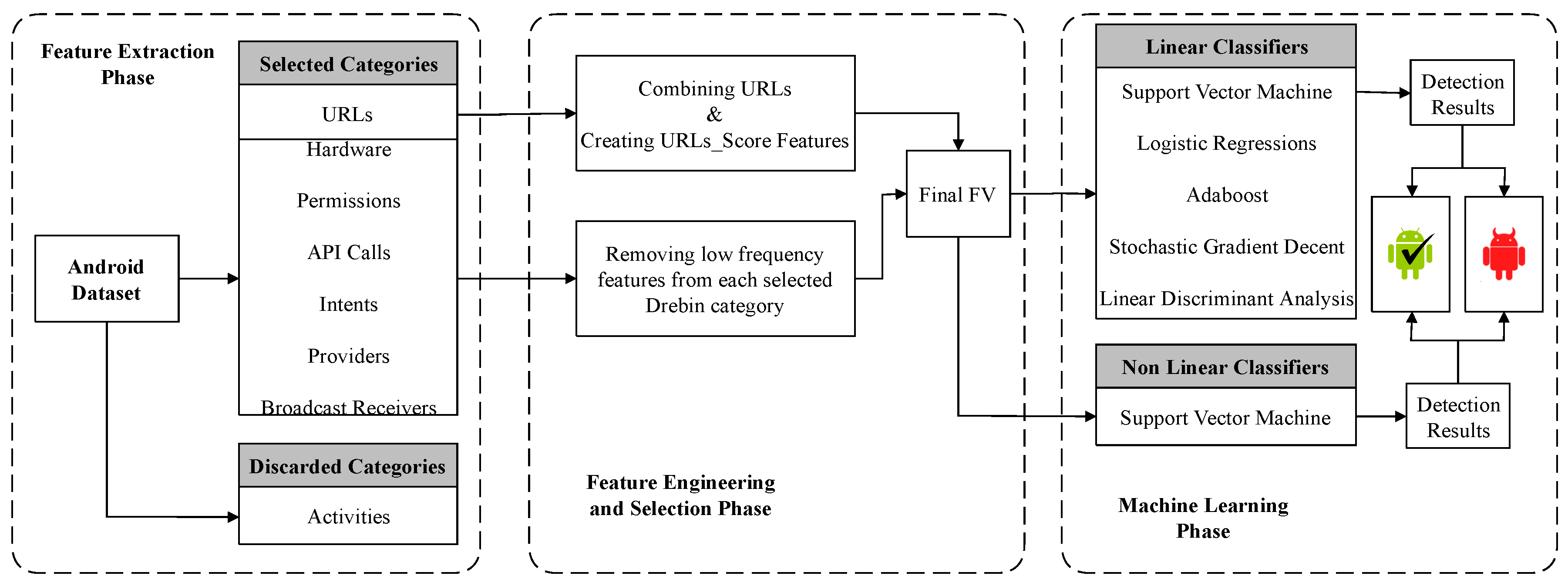
In [6], the authors proposed using the extracted URLs from the Drebin dataset as unique binary features. A feature value of zero indicated that an application did not include the specific URL being investigated; otherwise, the feature value was one. This treatment drastically increases the feature space of the dataset. Some methods treat URLs as redundant features and ignore this feature category [35].

In [36], the author proposed a method for analyzing Android application URLs and traffic. They collected and stored the traffic data for each URL from a set of benign and malware Android applications. Then, they analyzed the traffic to find any possible discriminative features of malware and benign applications. The proposed method achieved approximately 98.7% accuracy using the application URLs and network traffic only. The main issue with this method was that a considerable amount of traffic data must be collected before determining whether the application is benign or malware. Thus, some important information might be transferred or received during traffic collection. In addition, the tool ignored other important features, such as Android permissions, which may negatively affect the accuracy of the approach.

3. Methodology

The proposed system is composed of three phases: the feature extraction, feature engineering and selection, and ML model construction phases. The system block diagram is illustrated in Figure 1. In this section, we cover only the first two phases of selecting the most informative features, as we use the ML model (third phase) as it is.

3.1. Feature Extraction

We extracted the static features from the manifest and the disassembled dex code of the Android application. This information can be obtained by reading these two files. Then, we represent each Android application as a text file with one feature per line. The extracted features are similar to the extracted features described in [6], except we excluded those in the activity category.

3.2. Feature Engineering

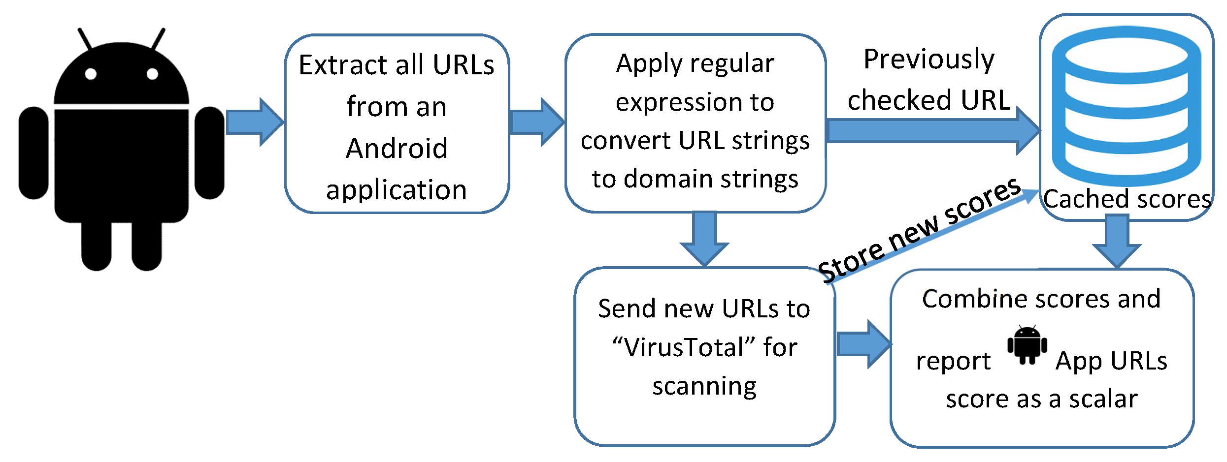
To construct the feature vector, we extract six categories of Android application features from the Android manifest file and source code. These feature types are Android permissions, used permissions application components, intent filters, and APIs (restricted and suspicious). We ignored features belonging to the activity category because many types of malware applications repack benign applications. Thus, the numbers of activity features considered malware and benign are almost the same.

Then, we merge all the application features belonging to the URL category into a single feature; this feature reflects the degree of maliciousness of all the URLs found in one application, and we call it the URL maliciousness score, or URL_score for short. Thus, we finally add the final feature to the feature vector.

URL Feature Merging

The URLs are extracted from the manifest file of the Android applications. The features in the URL category can be redundant. For instance, if an application includes ten URLs from the same domain, the state-of-the-art methods generate ten different features for all the applications of the dataset, using one-hot encoding as in [6,37]. It is assumed that these ten features belong to the same domain. Thus, if the domain is classified as a malicious domain, then the ten features have the same meaning. In this case, one feature can represent the other nine features. In addition, if a URL exists in one application, it will be included as a feature in the feature vector of each application. The value of this feature is zero if the URL appears in the application and one if it does not. There is a high probability that a URL that appears in one application will not appear in other applications in a dataset. Thus, the feature vector may include many zeros for the features that belong to the URL category, resulting in sparseness. Thus, in this study, all the application URLs are represented as a single value of the application maliciousness score.

The block diagram of the URL score calculation for an Android application is depicted in Figure 2. The procedure starts by extracting all the URLs from the application files. Then, these URLs are converted to the domain format using a regular expression.

Considering this URL https://www.youtube.com/abc, it is converted to www.youtube.com. Different webpages from the same domain should receive the same maliciousness score. Next, the procedure searches for the extracted domain in the cached database of domain scores. If the domain exists among the cached scores, then it receives a score. Otherwise, the domain is sent to VirusTotal [38] for scanning. VirusTotal scans the submitted URL with 67 different URL scanner engines. Then, for each URL, each application receives a score based on the number of malicious findings reported. The score varies from 1 to 67, and the higher the score is, the more malicious the application. Finally, the application takes the highest reported score between the cached score, if one exists, and VirusTotal score as the value of the URL_score feature.

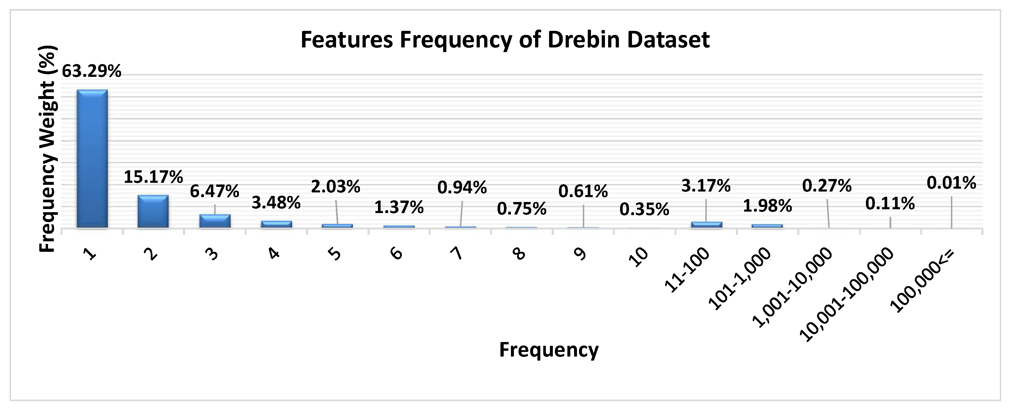
3.3. Feature Selection Based on the Feature Frequency

Inspired by the term frequency (TF) and inverse document frequency (IDF) techniques [39], we propose a frequency-based feature selection method called the feature frequency-application frequency ($FF-AF$) method. The core concept $FF-AF$ is that seldom used and highly frequent features are non-informative for the Android malware detection task or negatively affect the global performance of the task.

The TF-IDF technique measures two scores. First, the TF score is the number of occurrences of a word/term in a certain document divided by the total number of words in this document. Second, the IDF score is the number of documents containing a certain term, where N is the number of documents. The higher the IDF score is, the less the word is repeated in the N documents and the more important the word. Thus, this metric is called the IDF. In TF-IDF, words that are exclusive to a certain document can be used to recognize the document. Then, the TF-IDF weight is calculated as shown in Equation (1), where $n_{i,j}$ represents the number of occurrences of word i in document j, $M_j$ represents the total number of words in document j, N represents the number of documents, and $d{f}_i$ is the number of documents that contains term i.

$$w_{i,j}=\frac{n_{i,j}}{M_j}\times lg\left(\frac{N}{d{f}_i}\right)$$

(1)

To realize the TF-IDF method in the context of Android applications, we can replace the document with the Android application, and the words/terms with the extracted static features of this Android application. Thus, an Android application can be seen as a text file, where the dictionary includes the extracted feature names from the entire application dataset. Then, we use the binary $TF$ approach. The score $T{F}_{i,j}$ equals one if feature/term i belongs to application/document j, otherwise, the score $T{F}_{i,j}$ equals zero. We denote the feature space as $f_i\in F$, where F is the set of distinct features in the feature space and $f_i$ represents a unique feature. The intuition of using binary $TF$ is that it does not matter how many times the application uses a certain feature, e.g., a touch screen permission, but whether the Andoird application use this feature or not (0 or 1). In this context, we propose the $FF$ score, which corresponds to the $TF$ score. The $FF$ score is a binary value assigned to each distinct feature within the feature space, as described in Equation (2). Thus, if the feature space size is $\left|F\right|=S$, then each application receives as many as S $FF$ scores.

$$\begin{array}{c}F{F}_{i,j}=\left\{\begin{array}{c}1,feautreiappearsinapplicationj\hfill \\ 0,otherwise\hfill \end{array}\right.\end{array}$$

(2)

The $IDF$ score is used to assign a high score for seldom-occurring words in a given document. The ultimate goal of the TF-IDF method is to search for the document that best fits a set of keywords. In contrast, the task of malware detection involves finding common features for each benign and malware classes. We can assume that each class contains $N/2$ applications. Thus, if a feature appears in only one Android application out of $N/2$ applications, then this feature does not distinguish the class that contains that application. The goal of malware detection is to find the features that are common among all applications within the same class. Moreover, if a feature appears in N applications, then it is a useless feature because it appears in all feature sets within the two classes. Thus, if we have a new application with a feature that appears in N applications, then we cannot determine whether this new application belongs to the benign or malware class based on only this feature.

Thus, we replace the TF-IDF score with the proposed $FF-AF$ score, as shown in Equaion (3), where j represents the application number, i represents the feature number, and N represents the number of applications. Each feature out of S total features should receive an $FF-AF$ score. The $FF-AF$ score can be seen as the feature frequency, which is the number of applications containing this feature divided by the number of applications N. Using the $AF$ score, we do not need to apply the inverse concept of $IDF$. Instead, we use the $FF-AF\left(f_i\right)$ score to reflect how informative $f_i$ is. All $f_i$ features with $FF-AF\left(f_i\right)$ scores close to zero or 1 are considered non-informative and can be excluded from the feature space.

$$FF-AF\left(f_i\right)=\frac{{\sum }_{j=1}^{N}F{F}_{i,j}}{N}$$

(3)

Finally, we use the $FF-AF$ scores for frequency threshold-based feature selection. The threshold should be a range of $FF-AF$ scores that excludes seldom and common features close to zero and one. In other words, a set of features with $FF-AF$ scores less than a minimum threshold and a set of features with $FF-AF$ scores higher than a maximum threshold should both be excluded.

In addition, we propose two new measurements to evaluate the $FF-AF$ method. First, we propose measuring the weight of a given frequency in the feature space. For instance, this measurement can be used to determine how many features in the feature space have a frequency equal to one. This measure can help in determining the range of $FF-AF$ scores. The feature frequency is the numerator in Equation (3). Relative to the feature space size, if there are many features with a given frequency, then feature space will be greatly reduced if we exclude these features. We call this metric the frequency weight ($FW$). The $FW$ is calculated as shown in Equation (4), where $frequency$ represents a given frequency. This equation iterates over the entire feature space and counts only the features equal to the given frequency value.

$$FW\left(frequency\right)=\frac{{\sum }_{i=}^{\left|s\right|}\left\{\begin{array}{cc}1\hfill & ,frequency={\sum }_{j=1}^{N}F{F}_{i,j}\hfill \\ 0\hfill & ,otherwise\hfill \end{array}\right.}{\left|S\right|}$$

(4)

Second, we propose another measurement to evaluate the percentage of the feature space reduction for a given range of $FF-AF$ scores. We call this metric the frequency reduction percentage ($FRP$). The $FRP$ can be calculated using Equation (5), where min and max represent the minimum and maximum $FF-AF$ scores considered, respectively. The $FRP$ considers the number of features to be excluded from the feature space. Thus, Equation (5) iterates over all the $\left|S\right|$ features of the feature space and sums the total number of excluded features outside the $FF-AF$ score range. Then, the number of excluded features is divided by the total number of features.

$$FRP(min,max)=\frac{{\sum }_{i=}^{\left|s\right|}\left\{\begin{array}{cc}1\hfill & ,FF-AF\left(f_i\right)>min\hfill \\ 1\hfill & ,FF-AF\left(f_i\right)<max\hfill \\ 0\hfill & ,otherwise\hfill \end{array}\right.}{\left|S\right|}\times 100$$

(5)

4. Experimental Results

4.1. Experimental Setup

The experiments are performed on a computer with an Intel Xeon 1.70 GHz CPU E5-2609 v4 with 8 cores. The utilized OS is 64-bit Linux. Implementations are written in the Python programming language. We used the full Drebin dataset for training and testing the ML models. In all experiments, we used 30% of the data for testing and 70% for training.

All the classifiers’ attributes are set to the default values of the Python Scikit-learn package with the following exceptions. The SVM classifier’s kernel is set attribute is set to linear. The AdaBoost classifier’s number of estimator attribute is set to 30. The SGD classifier’s solver attribute is set to ’svd’. The logistic regression classifier’s C attribute is set to 1.0, penalty attribute is set to 12, and solver attribute is set to ’liblinear’. All the utilized classifiers class weight attribute is set to balanced, as the the two classes (i.e., malware and benign) are imbalanced.

4.2. Experimental Data

The Drebin dataset includes 123,453 benign and 5560 malware applications from 179 different malware families [6]. The Drebin dataset contains a total of 545,356 features, resulting in a feature vector with high sparsity. The number of applications in the Drebin dataset is 129,013. Thus, the Drebin dataset can be presented as a matrix of size 129,013 × 545,356. For this reason, the performance of nonlinear classifiers is not explored for the Drebin dataset because nonlinear classifiers are not applicable when the number of features is in the range of hundreds of thousands.

4.3. Results

4.3.1. Comparison against the Existing Malware Detection Methods

In

Table 1. Detection accuracy comparison.

Method	The Proposed Method	Ours (URL_Score)	Drebin [6]	CNN [40]	SVM [41]
Accuracy	99%	80%	94%	98%	98%
Num of features	349	1	545,356	545,356	545,356

, we compare the proposed method with three other methods. The numbers in bold in Table 1 indicates the best results. To the best of the authors’ knowledge, these methods are the only methods that used the complete Drebin dataset. These methods are the Drebin method [6], the CNN-based model proposed in [40], and an SVM model [41]. Information on the model disk size and training time was not available for the methods used in the comparison. Thus, the comparison included only the model accuracy and number of features. Intuitively, the greater the number of features is, the larger the model size. The model size depends on the number of features. Thus, the lower the number of features is, the smaller the model size. In Table 1, the 349 features are from the six feature categories (i.e., Android permissions, used permissions application components, intent filters, and APIs). Table 1 shows that the proposed method outperforms the existing methods in terms of accuracy and the number of features.

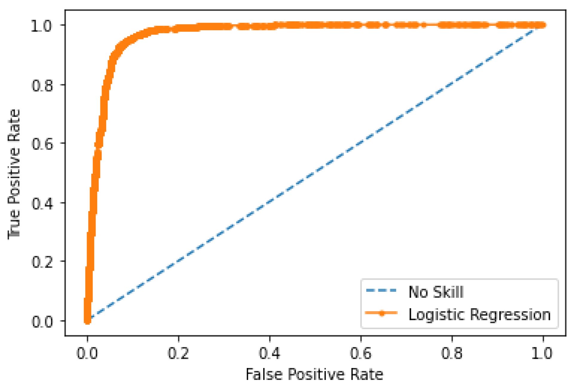
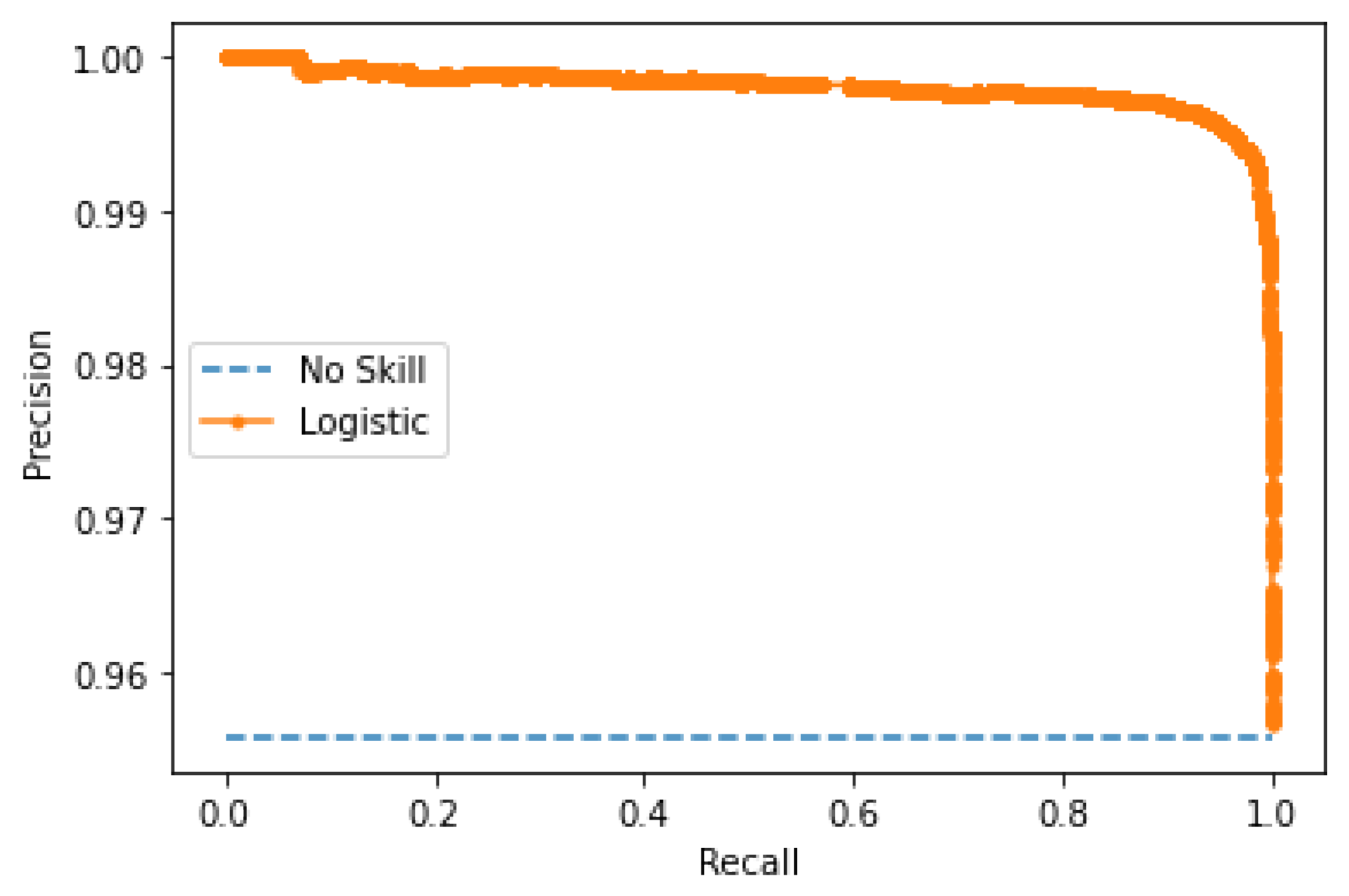
4.3.2. Accuracy Evaluation

Table 2. The test accuracy of the classification models on different feature spaces.

Feature Space	Linear SVM	Log. Reg.	AdaBoost	SGD	LDA
FS(1,1 × 105)	95.61%	95.68%	95.41%	95.71%	95.72%
FS(3,1 × 105)	95.71%	95.78%	95.81%	95.70%	95.75%
FS(5,1 × 105)	95.77%	95.70%	95.73%	95.75%	95.73%
FS(7,1 × 105)	98.94%	98.93%	97.95%	97.73%	98.83%
FS(9,1 × 105)	99.03%	98.82%	97.88%	97.77%	98.78%
FS(11,1 × 105)	98.89%	98.89%	97.90%	97.90%	98.73%
FS(13,1 × 105)	98.80%	98.78%	97.97%	97.80%	98.64%
FS(15,1 × 105)	98.77%	98.81%	97.98%	97.76%	98.54%
FS(25,1 × 105)	98.68%	98.62%	97.88%	97.87%	98.26%
FS(50,1 × 105)	98.44%	98.51%	97.86%	97.68%	98.18%
FS(75,1 × 105)	98.37%	98.45%	97.75%	97.62%	98.10%
FS(100,1 × 105)	98.47%	98.49%	97.85%	97.58%	98.18%
FS(125,1 × 105)	98.44%	98.50%	97.95%	97.50%	98.09%
FS(150,1 × 105)	98.04%	97.95%	97.73%	97.18%	97.78%
FS(250,1 × 105)	98.16%	98.40%	97.85%	97.54%	97.78%
FSURLs_score	80.15%	79.92%	79.89%	80.11%	79.67%

lists the accuracy of the linear classifiers for different feature spaces, $F{S}_{\left(min,max\right)}$. In addition, the feature space with a single feature, which is the URL_score, is denoted as $F{S}_{URL\_score}$. The results show that non-informative features, with low or high frequencies, act as noise, which degrades the classifier accuracy. Thus, the proposed method yields a lightweight size classifier. The linear classifiers listed in Table 2 exhibit similar performance, but linear SVM slightly outperforms the other linear classifiers.

Table 3. Average F1-score of the classification models.

Feature Space	Linear SVM	Log Reg.	AdaBoost	SGD	LDA
FS(3,1 × 105)	94%	94%	94%	94%	94%
FS(5,1 × 105)	94%	94%	94%	94%	94%
FS(7,1 × 105)	99%	99%	98%	98%	99%
FS(9,1 × 105)	99%	99%	98%	98%	99%
FSURLs_score	85%	85%	84%	85%	85%

lists the average F1 scores of the two Android application classes. Again, the results reflect similar performance for the utilized linear classifiers.

Finally, we evaluated the receiver operating characteristic (ROC) curve for the proposed logistic regression classifier on the FS_{(100,1 × 10⁵)}, as shown in Figure 3. The ROC area under curve (AUC) of Figure 3 is 97.1%. In addition, the precision-recall curve for the proposed logistic regression classifier on the FS_{(100,1 × 10⁵)} is depicted in Figure 4. The AUC value of Figure 4 is 99.8%. The other proposed classifiers show a similar behavior to Figure 3 and Figure 4.

In addition, we performed a cross-validation test using a 10-fold cross-validation approach [42]. This approach is computationally expensive but guarantees no waste of data. We performed the cross-validation test with the linear SVM only for $F{S}_{(9,1\times {10}^5)}$. The average reported accuracy for the ten tests was 97.82%. The lowest accuracy score was 96.93%, and the highest was 98.11%. The test results show that the model avoids the problem of overfitting.

4.3.3. Model’S Disk Size and Running Times

Table 4. The size of the classification models in bytes of $F{S}_9$.

Model Name	Linear SVM (URL) *	Linear SVM	Log_Reg	AdaBoost	SGD	LDA	Non Linear SVM
Model size	1	19,854	19,853	19,277	20,130	19,700	196,225,074

* The model utilized a feature vector of one feature, the proposed “URL_score”.

shows the size of the final classifier models in bytes to be stored in the external memory. This value reflects the complexity of the final model. The larger the model size is, the more complex the model and higher the classification time, and vice versa. For instance, the memory size of the linear SVM model is 20KB while the non-linear SVM model memory size is about 196MB. This result emphasizes the more complex the model is the more the memory size of the model.

The linear SVM training time is much shorter than that for the nonlinear SVM. For instance, linear SVM completed the training based on $F{S}_{(9,1\times {10}^5)}$ in 33 s and achieved an accuracy of 99%, and the nonlinear SVM completed the training based on the same feature vector in 4182 s, with an accuracy of 98%. For the same feature vector $F{S}_{(9,1\times {10}^5)}$, the fastest linear classifier to finish the training task were SGD at 11 seconds, and the slowest linear classifier was LDA, which needed 45 s to finish the training task.

4.3.4. Comparison against the Existing Feature Selection Methods

The proposed method was compared to the other feature selection methods. We selected the chi-square test for comparison. The chi-square test is a statistical test performed to measure the dependency of two variables. The chi-square test is applicable to categorical or nominal data. Chi-square reports a score for every feature, highlighting the relationship, if existent, between a certain feature and the target variable. Based on these scores, we use only the top k features to train the ML model.

The selection of the k values in the proposed work was based on

Table 5. The Drebin dataset features by frequency.

Feature Space	Drebin Original Feature Space	Drebin Modified Feature Space
	No. of Features	No. of Features	FRP
FS(1,1.3 × 105)	545,356	49,117	–
FS(3,1.3 × 105)	95,621	9838	20.0%
FS(5,1.3 × 105)	44,613	4890	9.9%
FS(7,1.3 × 105)	26,862	3253	6.6%
FS(9,1.3 × 105)	19,724	2411	4.9%
FS(11,1.3 × 105)	15,775	1888	3.8%
FS(13,1.3 × 105)	12,920	1544	3.1%
FS(15,1.3 × 105)	10,997	1380	2.8%
FS(25,1.3 × 105)	7223	865	1.8%
FS(50,1.3 × 105)	4269	517	1.1%
FS(75,1.3 × 105)	3112	352	0.7%
FS(100,1.3 × 105)	2422	349	0.7%
FS(200,1.3 × 105)	1313	172	0.4%

. For instance, using $F{S}_{(9,1\times {10}^5)}$ in the proposed method, we selected all features with frequencies equal to or greater than 9. The resultant feature space size was 19,724. To compare the chi-square and information gain methods with the proposed method, we set $k=\mathrm{19,724}$ in all the methods. Thus, all the methods consider the same number of features, but the selection criterion differs among methods. For the chi-square-based model, the best result for different feature spaces was FS(100,$1\times {10}^5$); utilizing this feature space, the best obtained accuracy and F1 score were 95.7% and 94%, respectively.

4.3.5. Evaluation of Feature Space Reduction

Table 6. Number of features of the Drebin dataset by category.

Category	URLs	Activity	Service Receiver	Intent	Provider	Permis.	Call	API Call	HW	Real Permis.
No. of features	310,511	185,729	33,222	6379	4513	3812	733	315	72	70

lists all the categories in the Drebin dataset and the number of features. Of note, the first two categories contain the largest numbers of features. The total feature space size of the Drebin dataset is 545,356, and we call this feature space the “original feature space”.

First, we studied the effect of URL merging into one feature, the URL_score, based on the Drebin dataset [6]. Table 6 shows that the URL feature category contains approximately 57% of all features. Thus, using the URL merging procedure reduced the 310,511 URL features to only one feature.

In addition, as discussed in Section 3.2, the features of the activity category can be excluded from the dataset without affecting the recognition of malware. Thus, 185,729 features are excluded from the 545,356 features in the Drebin dataset. Overall, 496,240 features (URL and activity features) were merged or excluded, and one feature was added. We call this feature space the “modified feature space”, and its size is $\left(545,356-496,240\right)+1=49,117$.

Second, we studied the effect of feature reduction using the proposed FF-AF score. Figure 5 depicts the feature frequencies with the corresponding FW values of the modified feature space. For instance, the feature space of the Drebin dataset includes 63.29% of features with a frequency equal to one. Figure 5 shows the FW values for frequencies 1 to 10. The FW scores are summed for frequencies from 11 to 100, 101 to 200 and so on due to space limits. For instance, if we exclude features with frequencies less than 3 and greater than 100,000, then the FF-AF minimum score is 3/129,013 and the maximum score is $\mathrm{100,000}/\mathrm{129,013}$. Thus, the feature space reduction equals $63.29+15.17+0.01=78.47\%$.

Table 5 lists the number of features filtered by frequency. The first column is the Drebin dataset feature space filtered by the frequency number, $F{S}_{\left(min,max\right)}$, where min and max represent the range boundaries of the feature frequencies. For instance, $F{S}_{\left(3,200\right)}$ is a feature space containing features with frequencies greater than two and less than 201. The dataset includes 129,013 samples; thus, the maximum frequency is the number of samples. Using an upper bound equal to $1.3\times {10}^5$, the resulting feature space includes all the features with frequencies higher than the lower bound of the range. The second and third columns of Table 5 list the size of the reduced feature space for the original and modified Drebin datasets, respectively. The features used in the classification belong to the intent provider, service, receiver, permission, API call, hardware, and real permission. In addition, all of the URL features are merged in one URL_score feature.

The last column of Table 5 represent the $FRP$ of the modified feature space. For instance, the $FRP$ of $F{S}_{\left(3,1.3\times {10}^5\right)}$ is calculated by dividing the number of features with frequencies within the range of $\left[3,1.3\times {10}^5\right]$ by the number of all features of the modified feature space, $FRP=\frac{9,838}{49,117}\simeq 20\%$. Thus, the feature space size of $F{S}_{\left(3,1.3\times {10}^5\right)}$ is about $20\%$ of the full modified feature space. We did not list the $FRP$ of the original feature space, as the used feature space in all the experiments is the modified feature space.

5. Conclusions

This research presented an evaluation of the detection of Android malware using ML classifiers based on the symmetric features of malware Android applications. The proposed approach aimed to produce a lightweight classifier model. To achieve this goal, we proposed reducing the number of features based on two methods. The first method includes removing the features with low and high frequencies and adding a new feature representing the URL maliciousness degree using URL scanning engines. The second method uses the chi-square method to select the most important k features, where k is the number of reduced features using the first proposed method. Using the Drebin dataset, the first method based on a linear SVM classifier achieves an accuracy of 99%, which is the highest reported accuracy to date for the full Drebin dataset, and the second method yields an accuracy of 95.74%. In addition, the proposed method yields a lightweight classifier with a size of 20KB in comparison to the 196MB required by the nonlinear SVM model. Thus, the proposed methods for reducing the feature space of the Android malware detection tasks significantly improve the accuracy, model memory size, and training time. The future work includes applying the proposed methods on the dynamic features of the Android applications. Thus, the proposed method can be used with any other static method to reduce the feature space and in turn, to reduce the feature extraction, training, and classification times.

References

1. Android OS Market Share of Smartphone Sales to End Users. 2018. Available online: https://www.statista.com/statistics/216420/global-market-share-forecast-of-smartphone-operating-systems/ (accessed on 3 December 2018).
2. Ribeiro, J.; Saghezchi, F.B.; Mantas, G.; Rodriguez, J.; Shepherd, S.J.; Abd-Alhameed, R.A. An Autonomous Host-Based Intrusion Detection System for Android Mobile Devices. Mob. Netw. Appl. 2020, 25, 164–172. [Google Scholar] [CrossRef]
3. Kim, D.; Shin, D.; Shin, D.; Kim, Y.H. Attack detection application with attack tree for mobile system using log analysis. Mob. Netw. Appl. 2019, 24, 184–192. [Google Scholar] [CrossRef]
4. Qiao, M.; Sung, A.H.; Liu, Q. Merging permission and api features for android malware detection. In Proceedings of the 2016 5th IIAI International Congress on Advanced Applied Informatics (IIAI-AAI), Kumamoto, Japan, 10–14 July 2016; pp. 566–571. [Google Scholar]
5. Kunda, D.; Chishimba, M. A survey of android mobile phone authentication schemes. Mob. Netw. Appl. 2018, 1–9. [Google Scholar] [CrossRef]
6. Arp, D.; Spreitzenbarth, M.; Hubner, M.; Gascon, H.; Rieck, K.; Siemens, C. DREBIN: Effective and Explainable Detection of Android Malware in Your Pocket. NDSS 2014, 14, 23–26. [Google Scholar]
7. Leeds, M.; Atkison, T. Preliminary Results of Applying Machine Learning Algorithms to Android Malware Detection. In Proceedings of the 2016 International Conference on Computational Science and Computational Intelligence (CSCI), Las Vegas, NV, USA, 15–17 December 2016; pp. 1070–1073. [Google Scholar]
8. Yuan, Z.; Lu, Y.; Xue, Y. Droiddetector: Android malware characterization and detection using deep learning. Tsinghua Sci. Technol. 2016, 21, 114–123. [Google Scholar] [CrossRef]
9. Ahmadi, M.; Sotgiu, A.; Giacinto, G. IntelliAV: Building an Effective On-Device Android Malware Detector. arXiv 2018, arXiv:1802.01185. [Google Scholar]
10. Wang, X.; Yang, Y.; Zeng, Y.; Tang, C.; Shi, J.; Xu, K. A novel hybrid mobile malware detection system integrating anomaly detection with misuse detection. In Proceedings of the 6th International Workshop on Mobile Cloud Computing and Services, Paris, France, 11 September 2015; pp. 15–22. [Google Scholar]
11. Moonsamy, V.; Rong, J.; Liu, S. Mining permission patterns for contrasting clean and malicious android applications. Future Gener. Comput. Syst. 2014, 36, 122–132. [Google Scholar] [CrossRef] [Green Version]
12. Dash, S.K.; Suarez-Tangil, G.; Khan, S.; Tam, K.; Ahmadi, M.; Kinder, J.; Cavallaro, L. Droidscribe: Classifying android malware based on runtime behavior. In Proceedings of the 2016 IEEE Security and Privacy Workshops (SPW), San Jose, CA, USA, 22–26 May 2016; pp. 252–261. [Google Scholar]
13. Somarriba, O.; Perez Ramos, L.C.; Zurutuza, U.; Uribeetxeberria, R. Dynamic DNS Request Monitoring of Android Applications via Networking. In Proceedings of the 2018 IEEE 38th Central America and Panama Convention (CONCAPAN XXXVIII), San Salvador, El Salvador, 7–9 November 2018; pp. 1–6. [Google Scholar]
14. Mao, K.; Capra, L.; Harman, M.; Jia, Y. A survey of the use of crowdsourcing in software engineering. J. Syst. Softw. 2017, 126, 57–84. [Google Scholar] [CrossRef] [Green Version]
15. Wang, W.; Zhao, M.; Wang, J. Effective android malware detection with a hybrid model based on deep autoencoder and convolutional neural network. J. Ambient. Intell. Humaniz. Comput. 2019, 10, 3035–3043. [Google Scholar] [CrossRef]
16. Tong, F.; Yan, Z. A hybrid approach of mobile malware detection in Android. J. Parallel Distrib. Comput. 2017, 103, 22–31. [Google Scholar] [CrossRef]
17. Xue, Y.; Zeng, D.; Chen, F.; Wang, Y.; Zhang, Z. A New Dataset and Deep Residual Spectral Spatial Network for Hyperspectral Image Classification. Symmetry 2020, 12, 561. [Google Scholar] [CrossRef] [Green Version]
18. Kabakus, A.T. What Static Analysis Can Utmost Offer for Android Malware Detection. Inf. Technol. Control. 2019, 48, 235–249. [Google Scholar] [CrossRef] [Green Version]
19. Amin, M.; Tanveer, T.A.; Tehseen, M.; Khan, M.; Khan, F.A.; Anwar, S. Static malware detection and attribution in android byte-code through an end-to-end deep system. Future Gener. Comput. Syst. 2020, 102, 112–126. [Google Scholar] [CrossRef]
20. Wang, K.; Song, T.; Liang, A. Mmda: Metadata Based Malware Detection on Android. In Proceedings of the 2016 12th IEEE International Conference on Computational Intelligence and Security (CIS), Wuxi, China, 16–19 December 2016; pp. 598–602. [Google Scholar]
21. Singh, B.; Evtyushkin, D.; Elwell, J.; Riley, R.; Cervesato, I. On the detection of kernel-level rootkits using hardware performance counters. In Proceedings of the 2017 ACM on Asia Conference on Computer and Communications Security, Abu Dhabi, UAE, 2–6 April 2017; pp. 483–493. [Google Scholar]
22. Idrees, F.; Rajarajan, M.; Conti, M.; Chen, T.M.; Rahulamathavan, Y. PIndroid: A novel Android malware detection system using ensemble learning methods. Comput. Secur. 2017, 68, 36–46. [Google Scholar] [CrossRef] [Green Version]
23. Feizollah, A.; Anuar, N.B.; Salleh, R.; Suarez-Tangil, G.; Furnell, S. Androdialysis: Analysis of android intent effectiveness in malware detection. Comput. Secur. 2017, 65, 121–134. [Google Scholar] [CrossRef] [Green Version]
24. Yerima, S.Y.; Sezer, S.; Muttik, I. Android malware detection: An eigenspace analysis approach. In Proceedings of the IEEE 2015 Science and Information Conference (SAI), London, UK, 28–30 July 2015; pp. 1236–1242. [Google Scholar]
25. Aafer, Y.; Du, W.; Yin, H. Droidapiminer: Mining api-level features for robust malware detection in android. In Proceedings of the International Conference on Security and Privacy in Communication Systems, Sydney, Australia, 25–28 September 2013; pp. 86–103. [Google Scholar]
26. Hou, S.; Ye, Y.; Song, Y.; Abdulhayoglu, M. Hindroid: An intelligent android malware detection system based on structured heterogeneous information network. In Proceedings of the 23rd ACM SIGKDD International Conference on Knowledge Discovery and Data Mining, Halifax, NS, Canada, 13–17 August 2017; pp. 1507–1515. [Google Scholar]
27. Garcia, J.; Hammad, M.; Malek, S. Lightweight, obfuscation-resilient detection and family identification of Android malware. ACM Trans. Softw. Eng. Methodol. (TOSEM) 2018, 26, 11. [Google Scholar] [CrossRef]
28. Wei, F.; Li, Y.; Roy, S.; Ou, X.; Zhou, W. Deep ground truth analysis of current android malware. In Proceedings of the International Conference on Detection of Intrusions and Malware, and Vulnerability Assessment, Bonn, Germany, 6–7 July 2017; pp. 252–276. [Google Scholar]
29. Zhou, Y.; Jiang, X. Dissecting android malware: Characterization and evolution. In Proceedings of the 2012 IEEE Symposium on Security and Privacy, San Francisco, CA, USA, 24–25 May 2012; pp. 95–109. [Google Scholar]
30. Andrototal Official Blog. Available online: http://blog.andrototal.org/ (accessed on 20 April 2020).
31. Liao, L.; Li, K.; Li, K.; Yang, C.; Tian, Q. UHCL-Darknet: An OpenCL-based Deep Neural Network Framework for Heterogeneous Multi-/Many-core Clusters. In Proceedings of the 47th International Conference on Parallel Processing (ICPP 2018), Eugene, OR, USA, 13–16 August 2018; p. 44. [Google Scholar]
32. Duan, M.; Li, K.; Li, K. An ensemble cnn2elm for age estimation. IEEE Trans. Inf. Forensics Secur. 2018, 13, 758–772. [Google Scholar] [CrossRef]
33. Ahmadi, M.; Sotgiu, A.; Giacinto, G. Intelliav: Toward the feasibility of building intelligent anti-malware on android devices. In Proceedings of the International Cross-Domain Conference for Machine Learning and Knowledge Extraction, Reggio, Italy, 29 August–1 September 2017; pp. 137–154. [Google Scholar]
34. Wang, X.; Zhang, J.; Zhang, A. Machine-Learning-Based Malware Detection for Virtual Machine by Analyzing Opcode Sequence. In Proceedings of the International Conference on Brain Inspired Cognitive Systems, Xi’an, China, 7–8 July 2018; pp. 717–726. [Google Scholar]
35. Li, C.; Zhu, R.; Niu, D.; Mills, K.; Zhang, H.; Kinawi, H. Android Malware Detection based on Factorization Machine. arXiv 2018, arXiv:1805.11843. [Google Scholar] [CrossRef]
36. Wang, S.; Chen, Z.; Yan, Q.; Ji, K.; Wang, L.; Yang, B.; Conti, M. Deep and Broad Learning based Detection of Android Malware via Network Traffic. In Proceedings of the 2018 IEEE/ACM 26th International Symposium on Quality of Service (IWQoS), Banff, AB, Canada, 4–6 June 2018; pp. 1–6. [Google Scholar]
37. Taheri, R.; Ghahramani, M.; Javidan, R.; Shojafar, M.; Pooranian, Z.; Conti, M. Similarity-based Android malware detection using Hamming distance of static binary features. Future Gener. Comput. Syst. 2020, 105, 230–247. [Google Scholar] [CrossRef] [Green Version]
38. VirusTotal. 2018. Available online: https://www.virustotal.com/ (accessed on 3 December 2018).
39. Robertson, S. Understanding inverse document frequency: On theoretical arguments for IDF. J. Doc. 2004, 60, 503–520. [Google Scholar] [CrossRef] [Green Version]
40. Grosse, K.; Papernot, N.; Manoharan, P.; Backes, M.; McDaniel, P. Adversarial perturbations against deep neural networks for malware classification. arXiv 2016, arXiv:1606.04435. [Google Scholar]
41. Shahpasand, M.; Hamey, L.; Vatsalan, D.; Xue, M. Adversarial Attacks on Mobile Malware Detection. In Proceedings of the 2019 IEEE 1st International Workshop on Artificial Intelligence for Mobile (AI4Mobile), Hangzhou, China, 24 February 2019; pp. 17–20. [Google Scholar]
42. Fushiki, T. Estimation of prediction error by using K-fold cross-validation. Stat. Comput. 2011, 21, 137–146. [Google Scholar] [CrossRef]
Figure 1. The proposed system block-diagram.
Symmetry 12 00858 g001
Figure 2. Block-diagram of the URLs score calculation procedure
Symmetry 12 00858 g002
Figure 3. The receiver operating characteristic (ROC) curve for the logistic regression model of feature space FS(100,1 × 10⁵).
Symmetry 12 00858 g003
Figure 4. The precision-recall curve for the logistic regression model of FS(100,1 × 10⁵).
Symmetry 12 00858 g004
Figure 5. Frequency weight (FW) scores for different features frequencies.
Symmetry 12 00858 g005