Construction and Optimization of Biconnected and Wide-Coverage Topology Based on Node Mobility

Abstract

Constructing a communications topology with fault tolerance and effective coverage plays an important role in wireless sensor networks. This paper is aimed at constructing and maintaining a biconnected topology, while minimizing the movement distance of the nodes and maximizing the coverage of the field of interest. First, it presents a new model with the motion constraint. If the nodes move at distance within the limit value calculated by the model, the topology is always connected, whether the neighbors of nodes are dynamic or static. Secondly, it improves the coverage strategy based on the nearest neighbor rule (NNR) and finds a rule of nodes’ spreading so that the nodes are distributed evenly and the spacing of the adjacent nodes is controllable. In addition, the nodes move only when necessary according to the added judgment conditions. Consequently, the movement distance is reduced. The simulation results prove the feasibility and effectiveness of the Localized Topology Optimized Method (LTOM) proposed by this paper. The connected indicators of the system’s topology during implementing LTOM are consistent, and the transformation of topology by LTOM is symmetric. Compared with the other distributed algorithm, NNR, LTOM reduces the movement distance of nodes, improves the connected probability, and maximizes the coverage of the topological structures under the biconnected conditions.

1. Introduction

Wireless mobile sensor networks are applied in multiple areas, such as rescue, exploration, visitation and reconnaissance. It has been widely concerned by scholars that intelligent agents, such as networked sensor or robots, can replace human beings to perform tasks in dangerous scenes [1,2]. Maintaining connectivity [3,4] and covering the field of interest [5,6] act as important supports and prerequisites for the multi-agent system (MAS) to perform a task. Therefore, to simultaneously build up a communications network with fault tolerance and a network widely covering the field of interest is an urgent problem in the research on multi-agent collaboration. In particular, networked agent nodes are often equipped with low-cost devices, as well as limited communications and energy resources. How to make these nodes move autonomously to optimize the topological structure of the system and reduce the moving energy consumption as much as possible still remains to be further studied.

The agent nodes exchange information through one or more hops in wireless networks. Any pair of nodes in the network can communicate with each other if and only if there is at least one communication path/link. $K$ can be defined as the number of disjoint communication paths between any pair of nodes. If the network is simply connected, namely $K=1$, the failure of one node will cause the whole network to be divided into two disconnected sub-networks. In the connected network of $K\ge 2$, if $K-1$, nodes are removed from the network, the network remains connected. However, with the larger $K$ value of the system and the denser nodes, it will impose greater motion constraints on the nodes system [7], which is not beneficial to enlarge the coverage of the system. Therefore, the objective of this paper is to construct and optimize the biconnected topological structure.

Building up the biconnected topological structure is an efficient approach to establish a communication network with destruction resistance [8,9]. The biconnected construction methods described in the existing literatures include the following three types [10]: 1. The transmitting power of each node in the system should be adjusted to build up the topological structure with destruction resistance [2,11,12,13], which is applicable for the node-intensive system. As for the node-sparse system, even though the transmitting power of each node reaches the maximum value, the system may not be biconnected. 2. Additional relay nodes should be deployed to improve the destruction resistance of the system [14,15], which can help solve the problem of topology control effectively. However, this method is not suitable for some conditions where the nodes cannot be deployed again. 3. It has been widely studied and applied that nodes can be moved to construct a biconnected topological structure [16,17,18]. Prithwish [16] proposed a centralized movement control method, which required the total information of the system. Then, in the literature [19], while maintaining the connectivity of the initial topological structure in the system, an iterative optimization algorithm was adopted to gradually move the nodes into the communications radius of the critical node. This method only requires the local information of k-hop neighbor nodes, which expends the application range, but the temporary cluster heads or central nodes are still necessary for calculating and controlling the movement of other nodes. Researchers [20] proposed a distributed algorithm based on node mobility to construct a biconnected topological structure, whereas, in a sparse topological system, this algorithm would lead to certain disconnections in the original topological structure. Thus, the authors in [10] put forward a model of motion constraints. The nodes move under the motion constraints, so as to avoid disconnections in the original topological structure. However, because this model was established under the relatively motionless conditions of the neighbor nodes, when the nodes and the neighbor nodes are in relative movements, some connections in the original topological structure will still be disconnected. Overall, further research is required on the optimization of the distributed topological structure based on node mobility.

Covering the field of interest is an important indicator for measuring the service quality of wireless sensor networks [21]. The coverage ability of a network usually refers to the increased area covered by nodes in an area and the reduced uncovered holes and redundant coverage area. In order to solve the problem of maximum coverage, scholars proposed many centralized methods [22,23], while others proposed distributed methods, among which the representative methods include the artificial potential field method [24], the Voronoi coverage method [25], and the nearest neighbor rule (NNR) [26], etc. However, it remains a challenge to minimize the movement distance while maintaining the nodes for effectively covering the field of interest. As the NNR algorithm is simple with the distributed features, this paper will enhance the solutions for the coverage based on the NNR algorithm.

Currently, many studies focus on minimizing the movement distance of nodes in the system while constructing the topological structure with destruction resistance [13] or minimizing the movement distance while solving the coverage problem [27]. On the other hand, few studies optimize multi-objective functions, including the construction of the topological structure with destruction resistance, the maximum coverage of the field of interest and the minimum movement distance [28]. In the literature [29], it is applicable for the node-intensive system to conserve the energy consumption while solving the problems of connectivity and coverage by scheduling. Literature [30] utilizes a centralized algorithm to solve the problems of connectivity, coverage and energy consumption. Literature [31] proposes a control model, which combines the control law of connectivity maintenance, with the control law of obstacle avoidance. In the literature [32], based on the above models, a control model introduced will solve the coverage problem, which aims to improve the invulnerability of communication networks, and enhance the coverage performance, and have the ability of obstacle avoidance. The above algorithm enables the multi-agent system to build up the expected topological structure autonomously, achieving the good results. However, it does not involve the minimum movement distance of nodes, and it requires the total information. This paper draws on the method of combining multiple control laws. Based on the local information of k-hop neighbor nodes, the nodes combine the biconnected construction method with the NNR coverage algorithm to construct the biconnected topological structure with the movement distance as short as possible and maximize the coverage under the biconnected condition.

This paper has made the following contributions to the construction and optimization of topological structure: (1) It proposes a new motion constraint model. If the node $v_i$ moves under the motion constraint condition, the node $v_i$ and the neighbor node (whenever static or dynamic) will always stay connected. (2) It improves the coverage method on the basis of NNR. The nodes in the system can be conducted in iterative optimization for the topological structure. In the end, the nodes will be distributed in the equal space and the node spacing is controllable. Besides, it adds constraints on node movement so that nodes can only move when it is necessary to reduce the movement distance. (3) It proposes a fully distributed approach for nodes moving autonomously to realize the multi objective optimization. Through this method of iterative optimization, the system can build up and maintain a biconnected topological structure while minimizing the movement distance of the nodes and maximizing the coverage of the field of interest.

Through the distributed strategy, this paper constructs the biconnected topological structure with maximum coverage. The sections of this paper are as follows: In Section 2, it describes the application background and related models. In Section 3, it refers to the exchange of location information between nodes and neighbor nodes and conduct the detection for the critical node. It also utilizes the nearest neighbor rule (NNR) to enhance coverage. In Section 4, in order to optimize the connectivity performance of nodes, nodes should accumulate near the critical node. As for optimizing the coverage performance, the nodes spread along a curve. Then, the nodes gradually optimize the topological structure by moving towards the resultant displacement at each iteration. In Section 5, it implements the simulation verification for the feasibility of the topological structure optimization algorithm. After optimization, the topological structure represents the features of low movement energy consumption, bi-connectivity and high coverage. In Section 6, it includes the summary and the expectations of future work.

2. Background and Nodes Distribution Model

2.1. Background

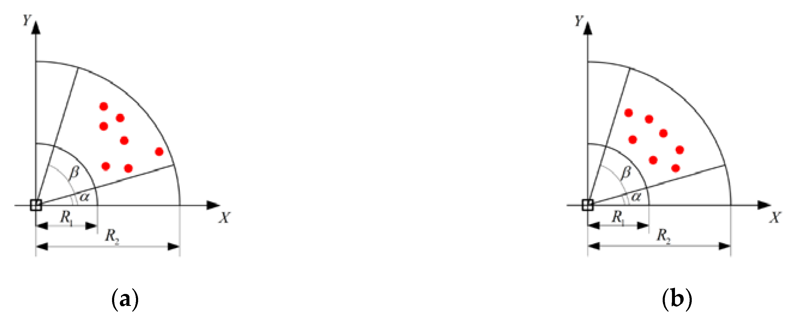
A number of small ground unmanned mobile platforms (hereinafter referred to as jamming nodes or nodes) with jamming equipment are scattered in the area near the enemy radar, as shown in Figure 1. When the radar is searching or tracing, the radar beam has directivity. Due to the directivity of the radar beam, effective jamming can be only achieved when interference energy enters from the main lobe of the radar beam. If the jamming nodes are deployed reasonably, no matter where the radar beam is directed, the jamming nodes in the main lobe of the radar beam can always be found to interfere with the radar, so that the jamming node group forms the jamming sector for the radar. Multi-jamming nodes can impose many-to-one co-interference on the radar, so that the radar detection performance is suppressed in the sector where the jamming node group is located.

At the initial time, the jamming nodes are randomly deployed in the sector region near the radar. The angle ${\theta }_i$ between the line linking the jamming node with the radar and the X-axis is the random variable uniformly distributed within the range of ($\alpha ,\beta$), and the distance from the jamming node to the radar, $R_i$, is the variable followed by the distribution function $f\left(r\right)=2r/\left(R_2^2-R_1^2\right)$, as shown in Figure 1a. In order to optimize the network topology, each node adopts a distributed strategy to move autonomously via iterative optimization, to construct a communications network with destruction resistance and topology with wide coverage, and to achieve the shortest average travelling distance. The distribution of nodes after the topology optimization is shown in Figure 1b.

2.2. Network Model and Coverage Model

Based on wireless communication theory, the maximum signal transmission distance is proportional to the transmission power. One node can be heard from the other if the transmission power of the other node is great enough. The distance of communication between each other is unique if the value of the transmission power is given. Thus, we use the distance instead of transmission power to represent the communication capability of the node. Besides, the network model is regarded as a Boolean model. That is, draw a circle with the position of node as the center and the communication distance as the radius. The nodes can communicate directly with each other if their corresponding circles are intersecting.

The assumptions are as follows: Nodes are isomorphic. The communication radius $r_c$ for each node is the same. Each node has the same interference performance, and each node $v_i$ knows its identification number $i$ and its exact coordinates $\left(x_i,y_i\right)$. At the same time, according to the previous reconnaissance radar information, the radar coordinates $\left(x_r,y_r\right)$ and the boundary value of the deployment area are available, as shown in Figure 1 $R_1,R_2,\alpha ,\beta$.

For the convenient description, the symbol definitions are as shown in

Table 1. Symbol definitions.

n	Number of the Jamming Nodes
$r_c$	Communication radius of the nodes
$\left(x_i,y_i\right)$	The coordinates of node $v_i$ in rectangular coordinates
${\theta }_i$	The angle between the line linking the node $v_i$ with the radar and the X-axis, called azimuth
$R_i$	The distance from the node to the radar
$\left[\alpha ,\beta \right]$	The combat zone is the sector area, and $\left[\alpha ,\beta \right]$ is the angle range of the combat zone, see Figure 1
$\left[R_1,R_2\right]$	The radial range of the combat zone, see Figure 1
$P\left(v_i,v_j\right)$	The sets of disjoint paths between the node $v_i and v_j$
$n_p\left(v_i,v_j\right)$	The number of the edges on the shortest path $P_1\left(v_i,v_j\right)$
$N\left(v_i\right)$	The sets of neighbor nodes for the node $v_i$
$△{\theta }_r$	The beam width of the radar main lobe, which is also the interval angle for dividing the subregions
$m$	Divide the combat zone into $m$ subregions
$S_i$	The subregion where the node $v_i$ is located
$△d_i\left(t\right)$	The moving distance of node $v_i$ at the $t$ iteration

:

The network of jamming nodes on the two-dimensional plane constitute graph $G=\left(V,E\right)$, among which $V=\left\{v_1,v_2,\dots ,v_n\right\}$ and $E=\left\{e_1,e_2,\dots ,e_m\right\}$ are the nodes set and the edges set, respectively. If the distance $d_{ij}$ between the node $v_i$ and the node $v_j$ is less than the communication radius, namely $d_{ij}<r_c$, there will be edge between the two nodes, otherwise there is no edge. Graph $G$ in this paper is an undirected graph. For the convenient description, the definitions are introduced as follows.

Definition 1.

K-connected. If there are at least K disjoint communication paths between any two nodes$v_i$and$v_j$, the Graph$G$is K-connected. Let$P\left(v_i,v_j\right)$be the sets of the disjoint communication paths between node$v_i$and node$v_j$. The definition of K-connected is as follows:

$$\left|P\left(v_i,v_j\right)\right|\ge K,\forall i,j\in \left[1,n\right].$$

When K = 1, Graph $G$ is simply connected. If there are $\mathrm{K}\ge 2$ disjoint paths in Graph $G$, when K-1 paths fail, Graph $G$ is still connected, which indicates that this network topology has fault tolerance and invulnerability. The connectivity and invulnerability of Graph $G$ will be better with a larger K, but excessive K requires more intensive nodes, causing network congestion or a higher cost. Therefore, this paper constructs a 2-connected network topology.

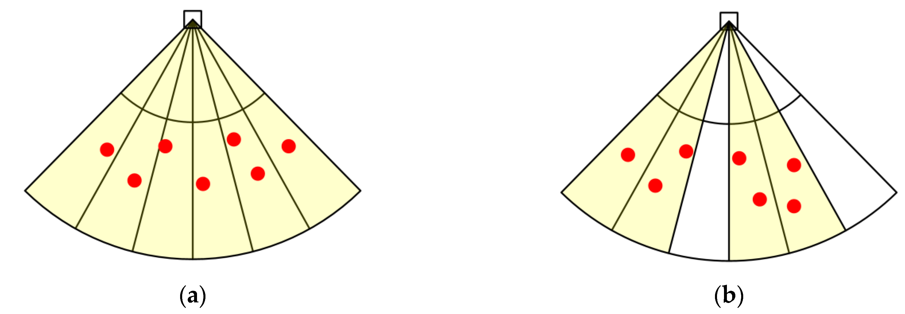
Definition 2.

Neighbor nodes. Let$P\left(v_i,v_j\right)$be the shortest paths linking$v_i$with$v_j$, and let$n_p\left(v_i,v_j\right)$be the number of the edges on the shortest path$P_1\left(v_i,v_j\right)$. Defining the set of nodes$N_{1hop}\left(v_i\right)$as 1-hop neighbors of the node$v_i$, the nodes in$N_{1hop}\left(v_i\right)$can communicate directly with the node$v_i$. Defining the set of nodes$N_{khop}\left(v_i\right)$as k-hop neighbors of the node$v_i$, there are k edges on the shortest path between the nodes in$N_{khop}\left(v_i\right)$and the node$v_i$. If there are no special explanations in this paper, the set of neighbors of the node$v_i$refers to 1-hop neighbor nodes.

$$N_{1hop}\left(v_i\right)=\left\{u\in V:n_p\left(v_i,u\right)=1\right\};$$

$$N_{khop}\left(v_i\right)=\left\{u\in V:n_p\left(v_i,u\right)=k\right\}.$$

Definition 3.

Coverage. It is assumed that all nodes located in the sector jamming area can implement the main lobe jamming to the radar, namely, when the radar beam points to the node, the single node has the ability to implement jamming to the radar. The main lobe width of the radar is$△{\theta }_r$the central angle range of the sector area is$\beta -\alpha$, and the sector area is divided into$m=\left(\beta -\alpha \right)/△{\theta }_r$subregions, as shown inFigure 2. If node$v_i$is located in a subregion, node$v_i$will cover this subregion, and the coverage area of node$v_i$is recorded as$S_i$. If there are nodes in each subregion, the sector region$S$will be completely covered, as shown inFigure 2a; otherwise, it will be not completely covered, as shown inFigure 2b. The mathematical description of the node for being completely covered is as follows:${\cup }_{i\in \left[1,n\right]}{S}_i=S$. The not completely covered mathematical description is as follows:$\exists S^{\prime }\in S$and$S^{\prime }\notin {\cup }_{i\in \left[1,n\right]}{S}_i$. The mathematical description of the coverage is as follows:

$$C=\frac{Area\left({\cup }_{i\in \left[1,n\right]}{S}_i\right)}{Area\left(S\right)}.$$

2.3. Objective Optimization Model

Each node moves gradually from the initial position to the position after topology optimization. This paper studies the optimization of the multi-objective function, namely minimizing the movement distance of nodes and maximizing the coverage, while building up the biconnected topological structure of the node network. The topology optimization of the node network can be described as shown in Formulas (1)–(3):

$$\min △D=\frac{1}{n}{\sum }_{i=1}^n{\sum }_{t=0}^T△d_i\left(t\right),$$

(1)

$$\max C,$$

(2)

$$\mathrm{s}.\mathrm{t}.,\left|P\left(v_i,v_j\right)\right|\ge 2,\forall i,j\in \left[1,n\right],$$

(3)

In Formula (1), $△D$ is the average movement distance of all the nodes, and $△d_i\left(t\right)$ is the distance that the node $v_i$ moves at the $t$ iteration. Formula (2) and Formula (3) are the definitions of coverage and bi-connectivity, respectively.

3. Critical Node Detection Algorithm and NNR Algorithm

3.1. Critical Node Detection Algorithm

It can be supposed that the system topology $G\left(V,E\right)$ is initially connected, if Graph $G$ is disconnected after a node in Graph $G$ and its affiliated edge deleted, this node is regarded as the critical node. Obviously, there is no critical node in the 2-connected topological structure. In order to construct a 2-connected topology, it requires detecting the critical node and then moving some nodes to make the critical node be a non-critical node, consequently making the initial 1-connected topological structure be 2-connected.

The depth-first search (DFS) method is often used for detecting the critical node. In the literature [15], it points out that the critical node has the following characteristics: Any node in Graph $G$ can be used as the root node to form the DFS tree. If a root node has two or more subtrees, this root node must be the critical node.

This paper detects the critical node through the distributed method [10]. Each node collects the information of the neighbor nodes and builds up the k-hop topological structure ($\mathrm{k}\ge 3$). The DFS algorithm is also used to detect whether the node is the critical node or not. If confirmed, the information of the critical node will be transmitted.

3.2. NNR

The multi-node deployment in this paper falls into the same category as the coverage of a wireless sensor network. To maximize coverage, the field of interest needs to reasonably adjust the node positions, as described in Definition 3. The traditional sensor network is intended to enhance the coverage ability of the network, which can increase the area covered by nodes in the area, reduce the uncovered holes and reduce the redundant coverage area. For the multi-node deployment problem in the scene of cooperative interference, the interference of nodes in the main lobe of radar beam performs well, while the radial distribution has little impact on the interference performance. Therefore, the multi-node coverage mainly refers to how to improve the coverage range of angle. The coverage performance of this paper means that the sector area is divided into several subregions by the radar beam, and the coverage performance will be better if more subregions are covered by nodes.

For a given number of nodes, if each node covers one subregion and each subregion has no redundant coverage, the nodes cover the sector area to the maximum extent. However, the minimized redundant coverage will cause an increase in node space, because when the nodes maximize the coverage area, they cannot form the biconnected communication or even maintain network connectivity due to the limited communication ability of nodes. Thus, the performance index of the node coverage algorithm is to maximize the node coverage under the condition of maintaining communication connectivity.

This paper applies the NNR algorithm to solve the coverage problem, as shown in Figure 3. Figure 3 indicates the process of node $v_i$ updating the positions at each iteration by using NNR. The specific steps are as follows:

• Node $v_i$ and the neighbor node exchange the information about their positions. Assume that the counter-clockwise direction is positive, the two nodes $v_l$ and $v_r,$ which are closest to node $v_i$ on the azimuth, are selected, namely ${\theta }_r<{\theta }_i<{\theta }_l$, and the azimuth of any other nodes $v_j$ is in accordance with ${\theta }_j<{\theta }_r$ or ${\theta }_j>{\theta }_l$.
• Calculate the angle that only involves the node $v_i$, then calculate the angular bisector of this angle, and the azimuth of the angular bisector is the azimuth ${\theta }_i\left(t+1\right)$ at the next time of the node. If the nodes $v_r$ and $v_l$ meet ${\theta }_r\left(t\right)<{\theta }_i\left(t\right)<{\theta }_l\left(t\right)$, ${\theta }_i\left(t+1\right)$ is the average value of the azimuth ${\theta }_l\left(t\right)$ and ${\theta }_r\left(t\right)$. If all neighbor nodes of $v_i$ are only at one side of the node, namely ${\theta }_i\left(t\right)<{\theta }_j\left(t\right)$ or ${\theta }_i\left(t\right)>{\theta }_j\left(t\right)$, and $v_j\in N\left(v_i\right)$, the virtual node $v_{vir}$ is constructed at the other side of the node $v_i$ and ${\theta }_i\left(t+1\right)$ is the average value of the azimuth between $v_l$ (or $v_r$) and $v_{vir}$, as shown in Formula (4). Moreover, the azimuth of the virtual node $v_{vir}$ is $v_{virr}=$ max{$\alpha ,\min \left\{{\theta }_j|v_j\in V\right\}-\Delta \theta$} or $v_{virl}=\min \left\{\beta ,\max \left\{{\theta }_j|v_j\in V\right\}+\Delta \theta \right\}$, among which $\Delta \theta$ is the control constant.

  $${\theta }_i\left(t+1\right)=\{\begin{array}{c}\frac{{\theta }_{virr}+{\theta }_l\left(t\right)}{2}, if v_i closest to boundary \alpha \\ \frac{{\theta }_r\left(t\right)+{\theta }_l\left(t\right)}{2},if there exists v_r and v_l\\ \frac{{\theta }_r\left(t\right)+{\theta }_{virl}}{2}, if v_i closest to boundary \beta \end{array}$$

  (4)
• Move the position ${\theta }_i\left(t\right)$ of node $v_i$ to the angular bisector ${\theta }_i\left(t+1\right)$, repeat the step 1 and 2 until ${\theta }_i\left(t\right)$ and ${\theta }_i\left(t+1\right)$ coincide.

NNR was originally used to solve the course consistency problem of multiple robots. Each node updates its own course according to the neighbor information, and the update formula is shown in Formula (5). Literature [33] proves the existence time $T_0$, and when $t=T_0$, all nodes have the same course ${\theta }_T$.

$${\theta }_i\left(t+T\right)=\frac{1}{1+N\left(V_i\left(t\right)\right)}\left({\theta }_i\left(t\right)+{\sum }_{j\in V_i\left(t\right)}{\theta }_j\left(t\right)\right),$$

(5)

The NNR mentioned above does not consider keeping the network connected. In Section 4, it adds motion constraints to maximize the coverage while maintaining the network connectivity.

4. The Optimization Method of the Topological Structure

The topology is optimized based on node mobility. Without loss of generality, the assumptions in terms of the motion model are as follows: (1) Each node knows its own position via GPS or a localization service, and acquires the position of its neighbors by communication. (2) The task area is free of obstacles. A node is able to choose an appropriate schedule to avoid collisions with other nodes. (3) The instantaneous model [34] is adopted. In this model, each node moves at a constant velocity, and is permitted to instantaneously change its velocity. That is, the acceleration is infinite, and each node can instantaneously accelerate to the constant velocity or instantaneously decelerate to zero velocity from the constant velocity.

4.1. The Limit Value for Moving

Due to the short communication radius, node $v_i$ moves in a certain direction subject to the neighbor node, $v_j$. If the movement distance exceeds the limit value, node $v_i$ will lose the connection with the neighbor node, $v_j$. Let ${\alpha }_{ijd}$ be the limit value in the direction of $\overrightarrow{d}$, and it denotes the maximum movement distance of node $v_i$ on the direction only under the constraint of its neighbor, $v_j\in N_{1hop}\left(v_i\right)$.

The current coordinate $\mathrm{I}\left(x_i,y_i\right)$ of node $v_i$ and the coordinate $\mathrm{J}\left(x_j,y_j\right)$ of the neighbor node is known. Based on the consistent rules, each node calculates the coordinates without constraints at the next time, namely the intentional destination coordinates ${\mathrm{I}}^{″}\left({x_i}^{″},{y_i}^{″}\right)$ and ${\mathrm{J}}^{″}\left({x_j}^{″},{y_j}^{″}\right)$. Due to communication constraints, the destination coordinates that the nodes can really reach are ${\mathrm{I}}^{\prime }\left({x_i}^{\prime },{y_i}^{\prime }\right)$ and ${\mathrm{J}}^{\prime }\left({x_j}^{\prime },{y_j}^{\prime }\right)$. Without the loss of generality, Figure 4 describes the planning graph of the node mobility.

There are four scenes where we calculate the limit value for moving.

Scene 1: It can be assumed that node $v_i$ and node $v_j$ move at the same speed to their respective destinations; when they move at a distance $l=l_i=l_j$, the spacing between node $v_i$ and node $v_j$ will reach the upper limit $r_c$, as shown in Figure 4. The equations can be listed according to the geometric relation between the nodes, see Equations (6) to (9).

$$l_i=l_j=l,$$

(6)

$${\mathrm{I}}^{\prime }\left(x_i^{\prime },y_i^{\prime }\right)=\mathrm{I}\left(x_i,y_i\right)+\frac{l_i}{\Vert {\mathrm{I}}^{″}\left(x_i^{″},y_i^{″}\right)-\mathrm{I}\left(x_i,y_i\right){\Vert }_2}\left({\mathrm{I}}^{″}\left(x_i^{″},y_i^{″}\right)-\mathrm{I}\left(x_i,y_i\right)\right),$$

(7)

$${\mathrm{J}}^{\prime }\left(x_j^{\prime },y_j^{\prime }\right)=\mathrm{J}\left(x_j,y_j\right)+\frac{l_j}{\Vert {\mathrm{J}}^{″}\left({x_j}^{″},{y_j}^{″}\right)-\mathrm{J}\left(x_j,y_j\right){\Vert }_2}\left({\mathrm{J}}^{″}\left({x_j}^{″},{x_j}^{″}\right)-\mathrm{J}\left(x_j,y_j\right)\right),$$

(8)

$$\Vert {\mathrm{I}}^{\prime }\left({x_j}^{\prime },{y_j}^{\prime }\right)-{\mathrm{I}}^{\prime }\left({x_j}^{\prime },{y_j}^{\prime }\right){\Vert }_2=r_c.$$

(9)

Solve the equations set and obtain the distance,

$$l=\left(\sqrt{B^2-4AC}-B\right)/2A,$$

(10)

where $A>0$, $C<0$, and B can be calculated from the known variables of $\mathrm{I}\left(x_i,y_i\right)$, $\mathrm{J}\left(x_j,y_j\right)$, ${\mathrm{I}}^{″}\left({x_i}^{″},{y_i}^{″}\right)$ and ${\mathrm{I}}^{″}\left({x_j}^{″},{y_j}^{″}\right)$.

Scene 2: As shown in Figure 5, the node $v_j$ only needs to move at a small distance. When node $v_j$ moves to the intentional destination ${\mathrm{I}}^{″}\left({x_j}^{″},{y_j}^{″}\right)$, the distance $l_{i^{\prime }{j}^{\prime }}$ between node $v_i$ and $v_j$ is still less than the communication radius $r_c$. At this time, the distance that the node $v_i$ is allowed to keep moving is $l_1.$ According to cosine theorem, $l_1$ satisfies Equation (11),

$$r_c^2=l_{i^{\prime }{j}^{\prime }}^2+l_1{}^2-2l_1\times l_{i^{\prime }{j}^{\prime }}\cos {\gamma }_1,$$

(11)

The solution of Equation (11) is as follows,

$$l_1=l_{i^{\prime }{j}^{\prime }}\cos {\gamma }_1+\sqrt{r_c^2-l_{i^{\prime }{j}^{\prime }}^2{\sin }^2{\gamma }_1},$$

(12)

Note that the value of variable $l$ in Scene 2 is $\Vert {\mathrm{J}}^{″}\left({x_j}^{″},{y_j}^{″}\right)-\mathrm{J}\left(x_j,y_j\right){\Vert }_2$. To avoid confusion with Equation (10) in Scene 1, $l$ satisfies the following definition,

$$l=\min \left\{\frac{\sqrt{B^2-4AC}-B}{2A},\Vert {\mathrm{J}}^{″}\left({x_j}^{″},{y_j}^{″}\right)-\mathrm{J}\left(x_j,y_j\right){\Vert }_2\right\}.$$

(13)

Scene 3: As shown in Figure 6, after node $v_i$ and node $v_j$ move at some distance $l$, if node $v_j$ continues to move, then $l_{i^{\prime }{j}^{\prime }}>r_c$; however, if node $v_i$ continues to move, the distance $l_{i^{\prime }{j}^{\prime }}$ between node $v_i$ and node $v_j$ is still less than the communication radius $r_c$. The distance that node $v_i$ can continue to move is $l_1$, as is solved in Equation (11), namely:

$$l_1=l_{i^{\prime }{j}^{\prime }}\cos {\gamma }_1+\sqrt{r_c^2-l_{i^{\prime }{j}^{\prime }}^2{\sin }^2{\gamma }_1}=2r_c\cos {\gamma }_1.$$

In Scene 2 and Scene 3, the process of node $v_i$ calculating the coordinate ${\mathrm{I}}^{\prime }\left({x_i}^{\prime },{y_i}^{\prime }\right)$ of the destination that the nodes can really reach is as follows: First, $l$ can be obtained from Formula (13). Then, assume that node $v_j$ stops, and that node $v_i$ continues to move, to judge whether the distance $l_{i^{\prime }{j}^{\prime }}$ between node $v_i$ and node $v_j$ exceeds $r_c$. If $l_{i^{\prime }{j}^{\prime }}<r_c$, then $l_1>0$, otherwise $l_1=0$. In Scene 1, Scene 2, and Scene 3, the maximum movement distance of the node $v_i$ is $l+l_1$.

Scene 4: As shown in Figure 7, node $v_j$ does not need to move or cannot move due to the constraints. Then, the movable distance of node $v_i$ is $l_2$, as is solved in Equation (11), namely:

$$l_2=l_{ij}\cos {\gamma }_2+\sqrt{r_c^2-l_{ij}^2{\sin }^2{\gamma }_2}.$$

In summary, the limit value of the node $v_i$ is,

$${\alpha }_{ijd}=\min \left\{l+l_1,l_2,\Vert {\mathrm{I}}^{″}\left(x_i^{″},y_i^{″}\right)-\mathrm{I}{\left(x_i,y_i\right)\Vert }_2\right\}.$$

(14)

Proposition 1.

The limit value of node$v_i$under the constraint of node$v_j$is${\alpha }_{ijd}$, and the limit value of node$v_j$under the constraint of node$v_i$is${\alpha }_{jid}$. Node$v_i$and node$v_j$respectively, move from the initial position to the destination. If the two nodes are initially connected, they will always remain connected when moving within the constraints’ limit value, that is, the connecting line$l_{i^{\prime }{j}^{\prime }}$between any point in the segment${\alpha }_{ijd}$and any point in the segment${\alpha }_{jid}$, is always less than or equal to the communication radius$r_c$.

Proof. 

If node $v_i$ and the neighbor node, $v_j$, move in the opposite directions, the distance between the nodes is monotone increasing, and spacing $l_{i^{\prime }{j}^{\prime }}$ reaches $r_c$ from small to large, so the spacing is $l_{i^{\prime }{j}^{\prime }}\le r_c$. If node $v_i$ and the neighbor node, $v_j$, move facing each other, the distance between the nodes firstly decreases and then increases to $r_c$. Thus, the spacing is also $l_{i^{\prime }{j}^{\prime }}\le r_c$. □

4.2. Building up the Biconnected Topology and Enhancing the Coverage Based on Mobility

This paper uses the basic rules of motion control of swarm intelligence, that is, the individuals keep together while avoiding collision with each other. In order to construct a biconnected network, the nodes move close to the critical node, and the displacement of the movement is $\Delta {\mathrm{X}}_{ic}$. To enhance the coverage performance, the node moves away from the neighbor nodes along the azimuth, and the next azimuth is ${\theta }_i\left(t+1\right)$. In order to maximize the angle coverage, when the node spacing exceeds the communication radius, the node moves to $R_i\left(t+1\right)$ along the radial as compensation. The resultant displacement of the node is as follows:

$$\Delta {\mathrm{X}}_i=\Delta {\mathrm{X}}_{ic}+\left\{R_i\left(t+1\right)\left[\cos \left({\theta }_i\left(t+1\right)\right),\sin \left({\theta }_i\left(t+1\right)\right)\right]-\left(x_i,y_i\right)\right\}.$$

(15)

Calculate the coordinate of the intentional destination ${\mathrm{I}}^{″}\left(x_i^{″},y_i^{″}\right)=\mathrm{I}\left(x_i,y_i\right)+\Delta {\mathrm{X}}_i$. The node is constrained by the connectivity of the neighbor nodes, and the limit value of the movement at the resultant displacement direction is ${\alpha }_i$, then the coordinate of the actual destination is as follows:

$$\mathrm{I}\prime \left(x_i^{\prime },y_i^{\prime }\right)=\mathrm{I}\left(x_i,y_i\right)+\Delta X_i^{\prime },$$

$$\Delta X_i^{\prime }=\frac{{\alpha }_i}{\Vert \Delta {\mathrm{X}}_i{\Vert }_2}\left({\mathrm{I}}^{″}\left(x_i^{″},y_i^{″}\right)-\mathrm{I}\left(x_i,y_i\right)\right).$$

(16)

4.2.1. Constructing the Biconnected Topology

Node $v_i$ detects the critical node according to Section 3.1. If there is one critical node in its neighbors, node $v_i$ moves toward the critical node. If there are multiple critical nodes, the node moves in the direction of the resultant displacement of the movement to the multiple critical nodes. From Figure 8, if the critical node, $v_c,$ and its attached edges are removed, the original topology is divided into a number of disconnected subgraphs. If all the neighbors of the critical node move within the $r_c/2$ distance range of the critical node, the spacing of all nodes is less than $r_c$, and the previously disconnected nodes become connected, thus turning the critical node into a non-critical node. The biconnected topology is formed.

The steps for node $v_i$ to construct the biconnected topology are as follows: First, detect whether this local node is the critical node, and receive the information from neighbors to verify whether the neighbor is a critical node. Then, verify whether the distance, $l_{icj}$, between the local node, $v_i$, and the critical node, $v_{cj}$, is greater than $r_c/2$. If it is true, node $v_i$ moves toward the critical node, $v_{cj}$. The movement displacement $\Delta {\mathrm{X}}_{icj}$ is as shown in Formula (17):

$$\{\begin{array}{c}\Delta {\mathrm{X}}_{icj}=w\times \left(\left(x_c,y_c\right)-\left(x_i,y_i\right)\right)\\ w=\left(1+\mathrm{sign}\left(l_{icj}-r_c/2\right)\right)/2\end{array},$$

(17)

where sign() is the sign function. If there are several critical nodes in the neighbors, node $v_i$ should calculate the resultant displacement of the movement to the multiple critical nodes, namely $\Delta {\mathrm{X}}_{ic}=\sum \Delta {\mathrm{X}}_{icj}$.

Each node has consistent calculation rules, which can predict the intentional destination coordinates at the next time of the neighbors without communication with the neighbors. It is suitable for distributed computing. In the meantime, the node only moves at a small distance to the point that is within the $r_c/2$ distance of the critical node. This operation reduces node mobility and saves energy consumption.

4.2.2. Enhancing Coverage

The system enhances the coverage performance according to NNR in Section 3.2. If node $v_i$ has the two nearest neighbors, $v_l$ and $v_r$, which meet the condition of ${\theta }_l\left(t\right)<{\theta }_i\left(t\right)<{\theta }_r\left(t\right)$, then the azimuth ${\theta }_i\left(t+1\right)$ at the next time of the node can be calculated by Formula (4). If all neighbors of node $v_i$ are only on one side of the node, the azimuth of the virtual node needs to be determined. This section introduces the control constant $\Delta \theta$ to determine the azimuth of the virtual node.

Proposition 2.

In the polar (or rectangular coordinate system) coordinate system, the multiple nodes spread along the$\theta$axis (X axis) according to NNR. Assume that node$v_i$is the outermost node in the multiple nodes system. Let$\Delta \theta$($\Delta X$) be the distance between node$v_i$and the virtual node on the$\theta$axis (X axis). If the area where the nodes system located is large enough, namely the width of the area is$\beta -\alpha >\left(n+1\right)\Delta \theta$, then the spacing of adjacent nodes on the$\theta$axis (X axis) will be$\Delta \theta$($\Delta X$) within finite iterations. If the nodes system is constrained by the area boundary, namely the width of the area is$\beta -\alpha <\left(n+1\right)\Delta \theta$, then the spacing of the adjacent nodes on the$\theta$axis (X axis) will be$\left(\beta -\alpha \right)/\left(n+1\right)$within finite iterations.

Proof. 

Studies [26,33] prove that $\forall v_i\in V$ the node spreads along the $\theta$ axis (X axis), and, for any given $\mathsf{\epsilon }$, there exists a time $t_k$, which makes $\left|{\theta }_i\left(t+1\right)-{\theta }_i\left(t\right)\right|<\mathsf{\epsilon }$ when $t>t_k$.

If the nodes system is not constrained by the space boundary, let $v_1$ and $v_{vir}$ be the outermost node and the virtual node, respectively, with spacing for $\Delta \theta$, and let $v_2$ be the nearest neighbor node of $v_1$, with spacing for $\Delta {\theta }_{12}$. It can be assumed that for any given $\mathsf{\epsilon }$, there exists a time $t_k$, which makes $\left|{\theta }_i\left(t+1\right)-{\theta }_i\left(t\right)\right|<\mathsf{\epsilon }$ when $t>t_k$, but $\Delta \theta \ne \Delta {\theta }_{12}$. Accordingly, ${\theta }_i\left(t+1\right)-{\theta }_i\left(t\right)=\frac{{\theta }_2\left(t\right)+{\theta }_{vir}\left(t\right)}{2}-{\theta }_i\left(t\right)=\left(\Delta \theta -\Delta {\theta }_{12}\right)/2\ne 0$. This assumption fails. Thus, within finite iterations, the spacing of adjacent nodes on the $\theta$ axis (X axis) is $\Delta \theta$.

If the nodes system is constrained by the region boundary, after a finite number of iterations, the spacing of adjacent nodes on the $\theta$ axis (X axis) is equal. That is, all nodes are evenly distributed along the $\theta$ axis (X axis), and the spacing is $\left(\beta -\alpha \right)/\left(n+1\right)$. □

After the distance constant $\Delta \theta$ determined, the nodes will eventually be evenly distributed along the $\theta$ axis (X axis), and the azimuth spacing of adjacent nodes is $\Delta \theta$. In order to effectively cover the radar scanning area, $\Delta \theta =\Delta {\theta }_r$ can be applied and $\Delta {\theta }_r$ is the main lobe beam width of the radar.

The nodes only spread in the direction of azimuth, which may lead to the disconnection of communication between the nodes, i.e., $l_{ij}>r_c$. In the meanwhile, nodes accumulate along the radial direction, then they can continue to expand the angle range in the azimuth direction. When the spacing between node $v_i$ and the nearest neighbor node, $v_{cn},$ is $l_{icn}>r_c/2$, or when the minimum angle between node $v_i$ and its neighbors is $\min \left({\theta }_{ij}\right)<\Delta {\theta }_r$ while the maximum radial spacing between node $v_i$ and its neighbors is $\max \left(R_{ij}\right)>r_c/2$, node $v_i$ needs to move in the radial direction. The radial coordinate $R_i\left(t+1\right)$ after movement is as follows:

$$\begin{array}{l}{R}_i\left(t+1\right)=\\ \{\begin{array}{cc}\hfill \left(\underset{j\in N_{1hop}\left(v_i\right)}{\max }{R}_j\left(t\right)+\underset{j\in N_{1hop}\left(v_i\right)}{\min }{R}_j\left(t\right)\right)/2,& l_{icn}>r_c/2 or \min \left({\theta }_{ij}\right)<\Delta {\theta }_r and \max \left(R_{ij}\right)>r_c/2\hfill \\ \hfill R_i\left(t\right),& otherwise\hfill \end{array}\end{array}.$$

(18)

4.2.3. Remove Redundant Connections

According to the contents of Section 4.1, the node $v_i$ calculates the motion limit value under the constraint of each neighbor. If the node mobility meets the constraints of all neighbors, it will be limited by redundancy, then the node cannot cover the radar scanning area to the maximum extent. Therefore, the node $v_i$ selects some neighbors to disconnect, while the topology remains biconnected.

The priority of disconnection with the neighbors should be determined. The level of the priority in disconnection will be higher with the smaller limit value. When the limit value remains the same, the level of the priority in disconnection will be higher with the longer distance.

Based on the critical node detection algorithm in Section 3.1, node $v_i$ verifies whether the neighbors are redundant one by one according to the order of disconnection priority from high to low. Assume that node $v_i$ is disconnected with neighbor $v_j$ and the neighbors with higher priorities, then verify whether a new critical node is created. If not, it indicated that neighbor $v_j$ is redundant and will be added to the set $dis\_req$. Otherwise, the critical node detection should be stopped. Let $dis\_re{q}_i$ be the redundant nodes set saved by node $v_i$.

It uses a handshake mechanism in which both the local node and neighbor confirm that they are ready to disconnect the communication. The process of the handshake mechanism is as follows: The node $v_i$ calculates and broadcasts the redundant nodes’ set $dis\_re{q}_i.$ At the same time, node $v_i$ receives the redundant nodes set $dis\_re{q}_j$ from the neighbors. When receiving the information from node $v_j$, the local node, $v_i$, verifies whether $v_j$ belongs to the redundant nodes’ set $dis\_re{q}_i$, and whether $v_i$ belongs to the redundant nodes’ set $dis\_re{q}_j$. If both the conditions are met, $v_i$ and $v_j$ can be disconnected and $v_j$ can be stored in the set $di{s}_i$.

The limit value of the node ${\mathrm{v}}_{\mathrm{i}}$ can be updated as follows:

$${\alpha }_i=\min \left\{{\alpha }_{ijd}\right\},v_j\in N_{1hop}\left(v_i\right)\backslash di{s}_i.$$

(19)

Solve Formula (4), (13) to (18), and the actual destination coordinate ${\mathrm{I}}^{\prime }\left(x_i^{\prime },y_i^{\prime }\right)$ of the node $v_i$ is obtained.

4.2.4. Termination of the Algorithm

The steps to optimize the topology for each node are summarized as follows:

• Obtain the position coordinate $\mathrm{I}\left(x_i,y_i\right)$ of the local node by GPS and obtain the position coordinates of its neighbors by communication.
• Calculate the actual destination coordinate ${\mathrm{I}}^{\prime }\left(x_i^{\prime },y_i^{\prime }\right)$ and move to the destination.
• Repeat Step 1 and Step 2 until ${\mathrm{I}}^{\prime }\left(x_i^{\prime },y_i^{\prime }\right)\approx \mathrm{I}\left(x_i,y_i\right),$ then the algorithm is terminated.

The topology optimization algorithm in this paper has the characteristics of starting at any time and ending at any time. Each iteration can be periodic. Even if a node does not move to the destination ${\mathrm{I}}^{\prime }\left(x_i^{\prime },y_i^{\prime }\right)$ at the end of a period, the coverage and connectivity performance of the algorithm will not be affected. On the other hand, if each iteration is not periodic, the calculation of the next iteration can start when the node receives the new coordinates from all neighbors. It can be seen that this method has good fault tolerance and distributed characteristics.

5. Simulation

We verify the feasibility of the Localized Topology Optimized Method (LTOM) proposed in this paper using Matlab software. This paper adopts the LTOM, NNR [27], Genetic [35], and Hungarian [30] algorithms to optimize the topology, then analyzes and compares the average movement distance, coverage and connectivity of two algorithms. When NNR is applied for each node, the azimuth ${\theta }_i\left(t+1\right)$ of the next position is calculated by Formula (4), and the radial distance, $R_i\left(t+1\right)$, of the next position is calculated by the following formula:

$$R_i\left(t+1\right)=\{\begin{array}{c}\frac{R_i\left(t\right)+R_l\left(t\right)}{2}, if v_i closest to boundary \alpha \\ \frac{R_i\left(t\right)+R_r\left(t\right)+R_l\left(t\right)}{3},if there exists v_r and v_l\\ \frac{R_i\left(t\right)+R_r\left(t\right)}{2}, if v_i closest to boundary \beta \end{array}.$$

(20)

It is noted that LTOM and NNR are the distributed algorithms, while Genetic and Hungarian are the centralized algorithms. Assume that a central node or base station knows the global information when Genetic and Hungarian algorithms applied, once the optimized topology is obtained, then the central node sends instructions to make all nodes moving directly from their initial positions to the final destinations.

Besides, the pre-defined destinations are needed when the Hungarian algorithm is applied. The topology optimization problem could be transferred to the assignment problem that is to assign exactly one node to one destination in such a way that the moving distance of all nodes is minimized. The pre-defined destinations are calculated by the following formula:

$$\{\begin{array}{cc}\hfill R_i\left(end\right)=\frac{1}{n}{\sum }_j{R}_j,& \forall v_j\hfill \\ \hfill \Delta {\theta }_{ik}=\frac{r_c}{2R_i\left(end\right)},& if v_i and v_k are the adjacent nodes\hfill \end{array}.$$

(21)

In the simulation for all algorithms, the combat zone is a sector area with an angle range of $\left[0°,120°\right]$ and the radial range of $\left[1,9\right]$. Without the loss of generality, the radial distance has no metric unit, and 1 represents a 1-unit distance. The communication radius of each node is 2. As the system nodes are randomly distributed in the sector area, the system may be divided into several disconnected subgroups. For the simplification of analysis, it can be assumed that the initial topology is simply connected. The simulation will not consider the signal attenuation and jam of the communication. It can be assumed that the radar main lobe beam width is $\Delta {\theta }_r=10°$, namely the angle coverage range of a single node is $10°$. Moreover, it can be assumed that the algorithm’s iteration period is $\mathrm{T}=1$, and the movement speed of the nodes is 0.01.

In order to study the impacts of system scale on results, this paper analyzes the average movement distance, coverage, and connectivity of the four algorithms under scenarios with different number of nodes. Let the number of nodes be $n=5,10,15,20,25,30$. The different scenarios include complete coverage and uncomplete coverage. As the initial deployment of the nodes is random, the results of each calculation are inconsistent. The results in this paper are the mean value calculated for 50 times.

5.1. Feasibility Analysis

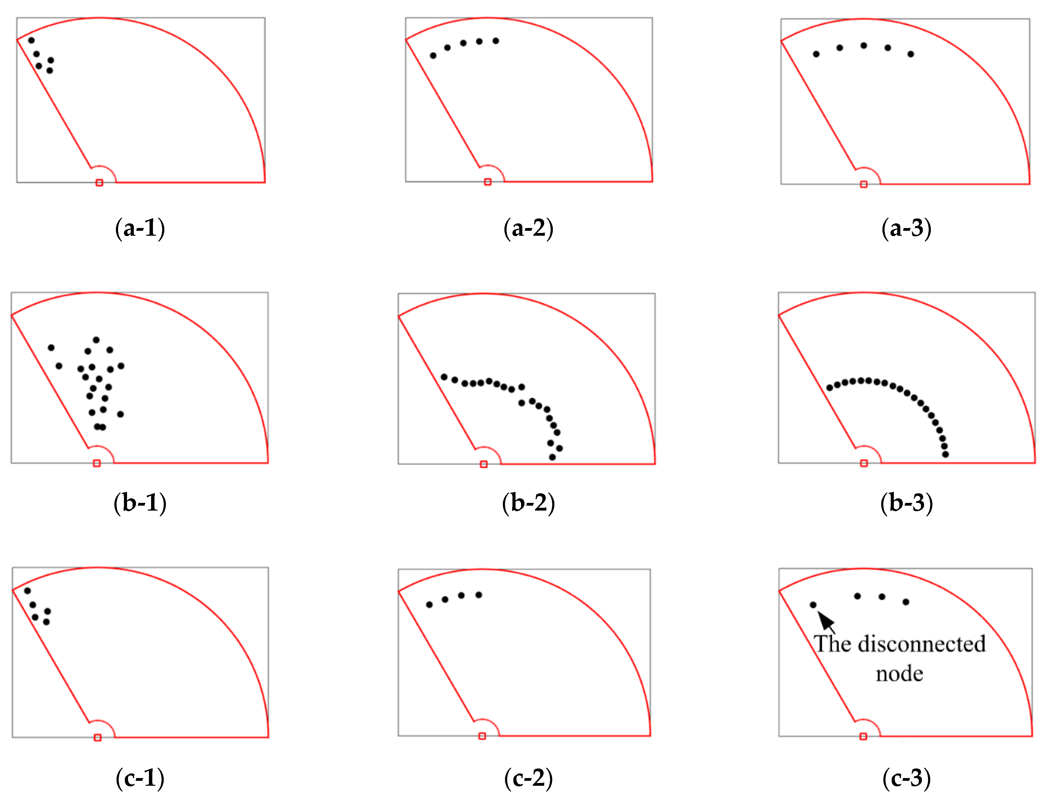
The simulation verifies the feasibility of the LTOM algorithm. Figure 9 describes the process of the system’s movement according to LTOM and NNR from the initial topology to the final topology under different scenarios. Scene 1 is as shown in Figure 9a-1–a-3, with the number of nodes at 5. Finally, the system of nodes cannot fully cover the sector area. Scene 2 is as shown in Figure 9b-1–b-3 with the number of nodes at 20. Finally, the system of nodes can fully cover the sector area. Scene 3 is as shown in Figure 9c-1–c-3. When one failure node appears, the system can be self-healing.

It can be seen from scene 1 that NNR has good coverage performance and maximizes the coverage without considering the connectivity constraints. LTOM integrates the NNR coverage algorithm and constructs the biconnected algorithm to maximize the coverage under the circumstance of maintaining 2-connectivity. However, it is constrained by the connectivity, and the coverage of LTOM is smaller than that of NNR. It can be seen from Scene 2 that the topology after NNR is an arc line where the nodes are evenly distributed. The nodes after LTOM are evenly distributed along the direction of the azimuth, but they are not at the same distance in the radial direction. The reason is that in order to reduce the movement distance of nodes, the LTOM algorithm adds constraint conditions when calculating the radial movement distance, and the nodes will only move radially if the constraints in Formula (17) are satisfied. Assume that the NNR algorithm also adds the constraint condition of this radial movement. Due to NNR not calculating the limit value of the connectivity constraint, when the condition of radial movement is not met, the nodes spread in the azimuth direction without radial accumulation as compensation, which is easy to disconnect the nodes, resulting in the original connected topology becoming disconnected. It can also be seen from Scene 3 that, for any connected system, LTOM can restore the system to 2-connectivity and maximize the coverage. The topology constructed by LTOM has the self-healing function when a node fails, and it indicates that the system enhances the destruction-resistance ability. For example, if the power of one node is too weak due to energy exhaustion that the node cannot work anymore, the optimized topology will be reconstructed by LTOM.

The symmetry of the multi-node system is shown in the invariance of the connectivity performance of the system’s topology after some transformations. The corresponding transformation is called a symmetric transformation. Let $\lambda$ be the algebraic connectivity of Graph $G$, and it can be calculated by the Laplacian matrix of $G$ from the algebraic graph theory. Define $f\left(G\right)=\mathrm{sign}\left(\lambda \left(G\right)\right)$ as the connected indicator, where $\lambda >0$ implies that $G$ is connected, and $\mathrm{sign}()$ is the sign function. The scenes show that the connected indicators of topology during implementing LTOM are consistent. Thus, the transformation of topology by LTOM is symmetric.

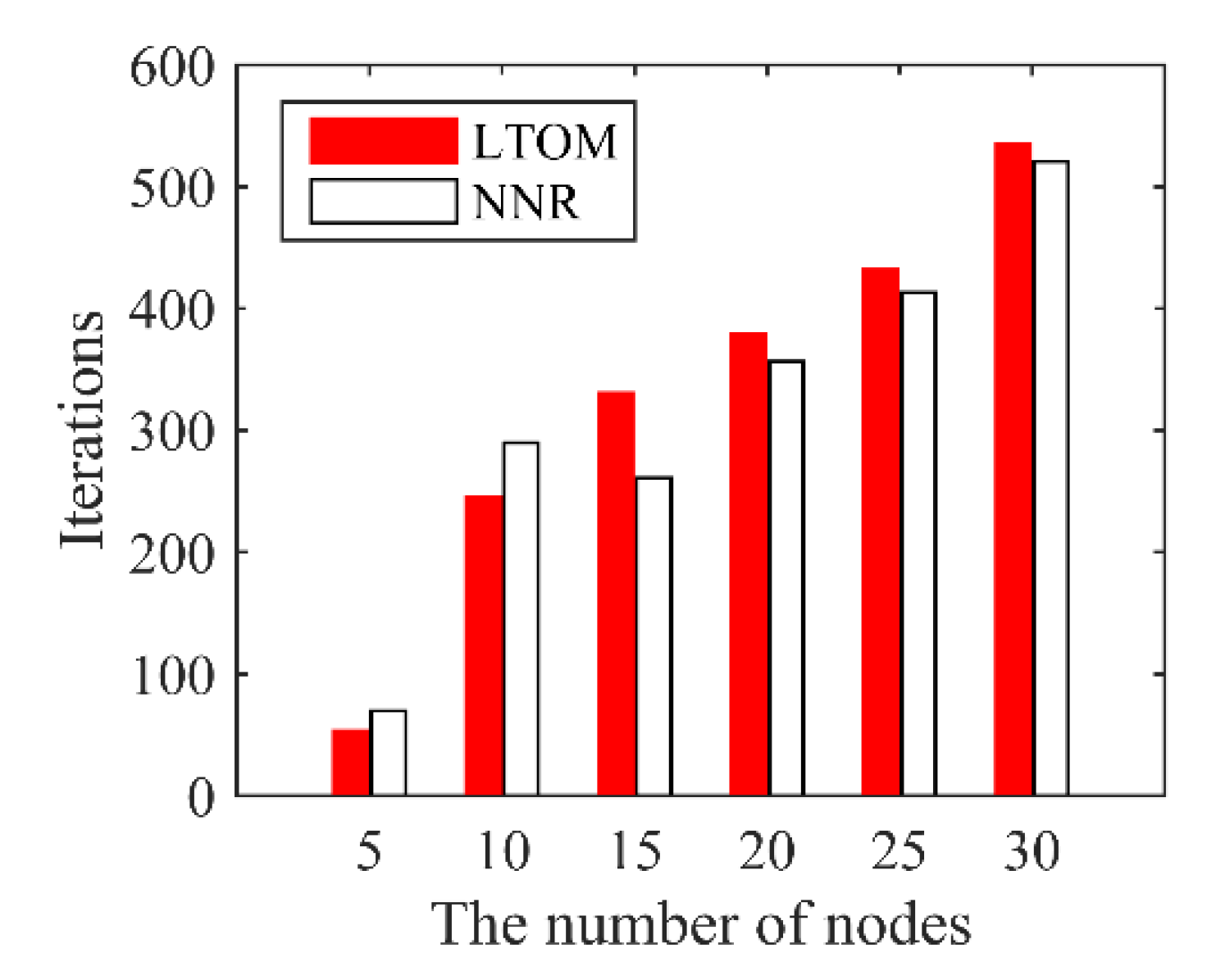
In LTOM and NNR, based on the local information, each node calculates iteratively the coordinates of position at next time and move gradually until the algorithms terminate. Figure 10 shows the iteration times of both algorithms over the number of nodes. The iteration times of LTOM is slightly higher than that of NNR when the number of nodes is more than 10. The reason is that the nodes move a short distance at each iteration for maintaining connected when LTOM is applied. The results illustrate that LTOM can terminate in the acceptable iteration times.

5.2. Performance Comparison

The LTOM, NNR, Genetic and Hungarian algorithms are operated under scenarios with a different number of nodes, and the simulation results are as shown in Figure 11, Figure 12 and Figure 13.

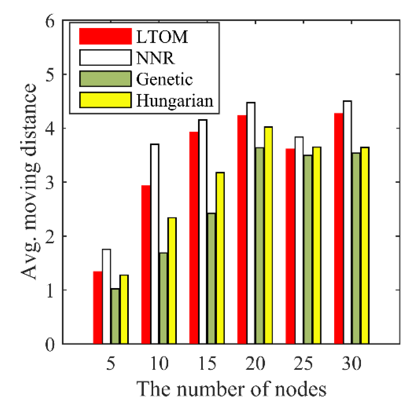
Figure 11 shows that the average movement distances of LTOM and NNR are greater than that of the Genetic and Hungarian algorithms. As mentioned, once the solutions are obtained by the Genetic and Hungarian algorithms, all nodes go straight to their destinations. However, when the distributed algorithms of LTOM and NNR are applied, the nodes adjust their destinations continuously and move step by step until the algorithms terminate. Although the centralized algorithms have better performance in terms of movement cost, they are impractical in some cases. For example, in scenarios where global information is not available in real time, when some nodes fail, the system can neither fill the coverage hole caused by the failure node nor reconstruct the biconnected topology.

Figure 11 shows that the average movement distance of LTOM is less than that of NNR under the scenarios with a different number of nodes. When the number of nodes goes from 5 to 20, the average movement distance of both algorithms is increasing. When the number of nodes goes from 20 to 30, the results of both algorithms vary irregularly and are basically consistent. When the number of nodes is small, the nodes system is not constrained by the area boundaries. The area covered by nodes increases as the number of nodes increases; accordingly, the movement distance of nodes increases. When the number of nodes is large, the nodes are constrained by the area boundaries, the movement distance no longer increases with the number of nodes.

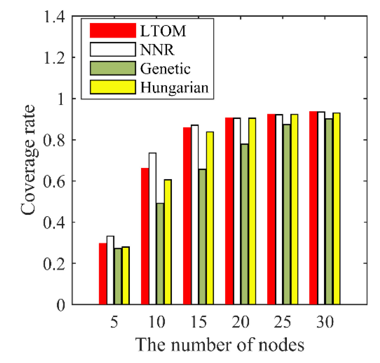
Figure 12 shows that the coverage rate of LTOM is smaller than that of NNR when the number of nodes ranges from 5 to 20, and the coverages of both algorithms are basically consistent when the number of nodes ranges from 20 to 30. Note that the topology after LTOM is biconnected; however, the connectivity after NNR cannot be guaranteed. In conclusion, the LTOM algorithm maximizes the coverage while the 2-connectivity is maintained. Besides, Figure 12 shows that the distributed algorithms of LTOM and NNR have better performance in terms of coverage than the centralized algorithms of Genetic and Hungarian.

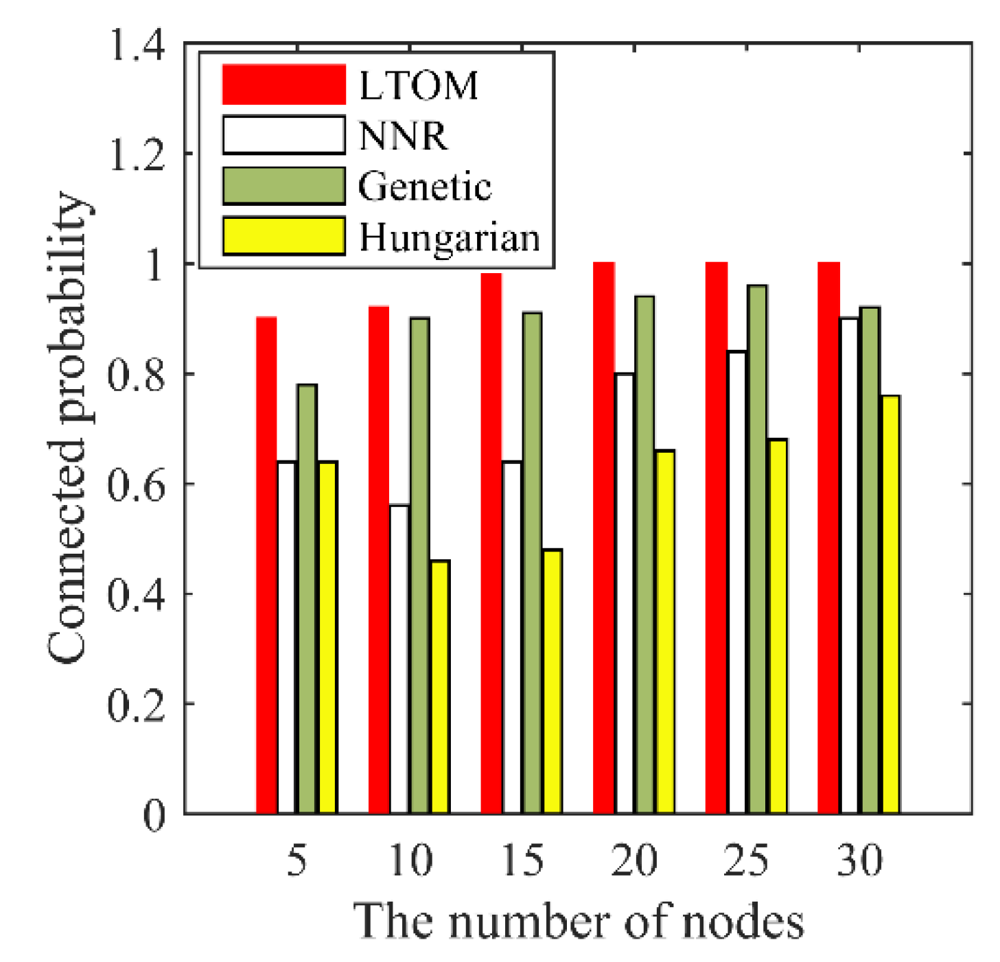
Connectivity is one of the main indicators to evaluate the invulnerability of topology. The connectivity in this paper is measured by the connectivity probability. The connectivity probability refers to the probability that the nodes system stays connected from any initially connected topology to the final topology, even in the presence of some node failures. Define the set of specific times $t=\left[20,60,100,140\right]$ to be the failure times. The connectivity probability is the ratio of the counting of surviving connected network to the total simulations in the presence of failures. Figure 13 shows that the connectivity probability of LTOM is the highest among all algorithms. The results show that the LTOM algorithm improves the performance of the connectivity by constructing a biconnected topology.

6. Conclusions

This paper proposes a new topology optimization method (LTOM), combining the biconnected construction algorithm and NNR coverage algorithm. The multi-objective optimization problem is solved, that is, to minimize the moving distance, to maximize the coverage, and to construct and maintain the biconnected topology. Applying LTOM only needs information from finite neighbors, which has the advantage of distributed computing. It is noticed that LTOM is not only applied to the scenario of radar countermeasure, but is also applied to other scenarios such as border surveillance or intrusion detection.

In terms of building up the biconnected topology, the limit value for moving is calculated. The topology stays connected whenever the nodes are moving or stationary according to LTOM. Meanwhile, the handshake mechanism is adopted to remove redundant connections. This mechanism reduces the impact of movement restrictions, and it maximizes the coverage without weakening the connectivity performance. In terms of improving the coverage, LTOM further optimizes the coverage strategy based on NNR. This paper discovers the rule of nodes spreading in an unbounded scenario. Let $\Delta \theta$ be the distance between the outermost node and the virtual node. The nodes after LTOM are distributed evenly, and the spacing of the adjacent nodes is $\Delta \theta$. Besides, the judgment is added to determine whether a node requires to move in the radial direction. The improved coverage strategy conduces to reduce the moving distance and energy consumption of the nodes system.

The feasibility and effectiveness of LTOM are demonstrated through simulation. For any initially connected topology, LTOM has the ability to construct a biconnected topology while the coverage is maximized. Compared with the other existing algorithms, LTOM in a decentralized way reduces the moving distance of each node, improves the performance of connectivity, and maximizes the coverage on the premise of bi-connection.

The LTOM algorithm optimizes the topology where the nodes are isomorphic. In future work, we will study how to optimize the topology while minimizing the cost in the case of inconsistent communication distances or different agents’ capabilities.

References

1. Tomic, T.; Schmid, K.; Lutz, P.; Domel, A.; Kassecker, M.; Mair, E.; Grixa, I.L.; Ruess, F.; Suppa, M.; Burschka, D. Toward a fully autonomous UAV: Research platform for indoor and outdoor urban search and rescue. IEEE Robot. Autom. Mag. 2012, 19, 46–56. [Google Scholar] [CrossRef] [Green Version]
2. Deniz, F.; Bagci, H.; Korpeoglu, I.; Yazici, A. An adaptive, energy-aware and distributed fault-tolerant topology-control algorithm for heterogeneous wireless sensor networks. Ad Hoc Netw. 2016, 44, 104–117. [Google Scholar] [CrossRef] [Green Version]
3. Ye, W.; Vaughan, R.T.; Sukhatme, G.S.; Heidemann, J.S.; Estrin, D.; Mataric, M.J. Evaluating control strategies for wireless-networked robots using an integrated robot and network simulation. In Proceedings of the IEEE International Conference on Robotics and Automation, Seoul, Korea, 21–26 May 2001; pp. 2941–2947. [Google Scholar]
4. Wang, S.G.; Mao, X.F.; Tang, S.J.; Li, X.Y.; Zhao, J.Z.; Dai, G.J. On movement-assisted connectivity restoration in wireless sensor and actor networks. IEEE Trans. Parallel Distrb. Syst. 2011, 22, 687–694. [Google Scholar] [CrossRef] [Green Version]
5. Yoon, Y.; Kim, Y.-H. An efficient genetic algorithm for maximum coverage deployment in wireless sensor networks. IEEE Trans. Cybern. 2013, 43, 1473–1483. [Google Scholar] [CrossRef] [PubMed]
6. Nguyen, T.G.; So-In, C.; Nguyen, N.G.; Phoemphon, S. A novel energy-efficient clustering protocol with area coverage awareness for wireless sensor networks. Peer Peer Netw. Appl. 2017, 10, 519–536. [Google Scholar] [CrossRef]
7. Wang, Q.; Chen, J.; Fang, H. Fault-tolerant topology control algorithm for mobile robotic networks. Int. J. Control Autom. 2014, 12, 582–589. [Google Scholar] [CrossRef]
8. Chen, L.; Liang, J.; Hu, Z.; Wu, B. Movement control algorithm of fault-tolerant UAVs Ad Hoc Networks. J. Natl. Univ. Def. Technol. 2012, 33, 58–62. [Google Scholar]
9. Shi, Y.; Sun, H.; Sheng, M.; Li, J.; Li, X. Constructing a robust topology for reliable communications in multi-channel cognitive radio Ad Hoc Networks. IEEE Commun. Mag. 2018, 56, 172–179. [Google Scholar] [CrossRef]
10. Guo, Q.; Yan, J.; Xu, W. Localized fault tolerant algorithm based on node movement freedom degree in flying Ad Hoc Networks. Symmetry 2019, 11, 106. [Google Scholar] [CrossRef] [Green Version]
11. Chang, Y.C.; Yuan, X.B.; Li, B.; Niyato, D.; Al-Dhahir, N. A joint unsupervised learning and genetic algorithm approach for topology control in energy-efficient ultra-dense wireless sensor networks. IEEE Commun. Lett. 2018, 22, 2370–2373. [Google Scholar] [CrossRef]
12. Bagci, H.; Korpeoglu, I.; Yazıcı, A. A distributed fault-tolerant topology control algorithm for heterogeneous wireless sensor networks. IEEE Trans. Parallel Distrb. Syst. 2015, 26, 914–923. [Google Scholar] [CrossRef]
13. Li, X.; Cai, J.; Zhang, H. Topology control for guaranteed connectivity provisioning in heterogeneous sensor networks. IEEE Sens. J. 2016, 16, 5060–5071. [Google Scholar] [CrossRef]
14. Nitesh, K.; Jana, P.K. Relay node placement with assured coverage and connectivity: A jarvis march approach. Wirel. Pers. Commun. 2018, 98, 1361–1381. [Google Scholar] [CrossRef]
15. Wang, Q.; Chen, J.; Fang, H. A construction method of fault-tolerant topology for multi-agent systems. Pattern Recognit. Artif. Intell. 2014, 27, 356–362. [Google Scholar]
16. Basu, P.; Redi, J. Movement control algorithms for realization of fault tolerant Ad Hoc Networks. IEEE Netw. 2004, 18, 36–44. [Google Scholar] [CrossRef]
17. Song, X.; Zhou, L.; Zhao, H. Localized fault tolerant and connectivity restoration algorithms in mobile wireless Ad Hoc Network. IEEE Access 2018, 6, 36469–36478. [Google Scholar] [CrossRef]
18. Vahid, K.A.; Orhan, D. TAPU: Test and pick up-based k-connectivity restoration algorithm for wireless sensor networks. Turk. J. Electr. Eng. Comput. Sci. 2019, 27, 985–997. [Google Scholar]
19. Chakraborty, N.; Sycara, K. Reconfiguration algorithms for mobile robotic networks. In Proceedings of the IEEE International Conference on Robotics and Automation (ICRA), Anchorage, AK, USA, 3–8 May 2010; pp. 5484–5489. [Google Scholar]
20. Das, S.; Liu, H.; Nayak, A.; Stojmenovi, I. Localized algorithm for bi-connectivity of connected mobile robots. Telecommun. Syst. 2009, 40, 129–140. [Google Scholar] [CrossRef]
21. Das, S.; Sahana, S.; Das, I. Energy efficient area coverage mechanisms for mobile Ad Hoc Networks. Wirel. Pers. Commun. 2019, 107, 973–986. [Google Scholar] [CrossRef]
22. Chang, Y.C.; Yuan, X.B.; Li, B.Q.; Niyato, D.; Al-Dhahir, N. Machine-learning-based parallel genetic algorithms for multi-objective optimization in ultra-reliable low-latency WSNs. IEEE Access 2019, 7, 4913–4926. [Google Scholar] [CrossRef]
23. Gupta, G.P.; Jha, S. Biogeography-based optimization scheme for solving the coverage and connected node placement problem for wireless sensor networks. Wirel. Netw. 2019, 25, 3167–3177. [Google Scholar] [CrossRef]
24. Huang, C.; Li, W.; Xiao, C.; Liang, B.; Han, S. Potential field method for persistent surveillance of multiple unmanned aerial vehicle sensors. Int. J. Distrib. Sens. Netw. 2018, 14, 1–13. [Google Scholar] [CrossRef] [Green Version]
25. Breitenmoser, A.; Schwager, M.; Metzger, J.C.; Siegwart, R.; Rus, D.L. Voronoi coverage of non-convex environments with a group of networked robots. In Proceedings of the IEEE International Conference on Robotics and Automation (ICRA), Anchorage, AK, USA, 3–8 May 2010; pp. 4982–4989. [Google Scholar]
26. Luo, J.; Ren, X.; Zou, S. A decentralized K-barriers construction approach based on nearest neighbors rule for two-dimensional rectangular region. Wirel. Netw. 2018, 24, 969–979. [Google Scholar] [CrossRef]
27. Nguyen, T.G.; So-In, C. Distributed deployment algorithm for barrier coverage in mobile sensor networks. IEEE Access 2018, 6, 21042–21052. [Google Scholar] [CrossRef]
28. Tripathi, A.; Gupta, H.; Dutta, T.; Mishra, R.; Shukla, K.K.; Jit, S. Coverage and connectivity in WSNs: A survey, research issues and challenges. IEEE Access 2018, 6, 26971–26992. [Google Scholar] [CrossRef]
29. Diya, T.; Rajan, S.; Mehmet, O.; Michael, H.; Wei, N. Energy-efficient military surveillance: Coverage meets connectivity. IEEE Sens. J. 2019, 19, 3902–3911. [Google Scholar]
30. Liao, Z.; Wang, J.; Zhang, S.; Cao, J.; Min, G. Minimizing movement for target coverage and network connectivity in mobile sensor networks. IEEE Trans. Parallel Distrb. Syst. 2015, 26, 1971–1983. [Google Scholar] [CrossRef] [Green Version]
31. Ghedini, C.; Ribeiro, C.H.C.; Sabattini, L. A decentralized control strategy for resilient connectivity maintenance in multi-robot systems subject to failures. In Proceedings of the International Symposium on Distributed Autonomous Robotic Systems (DARS), London, UK, 7–9 November 2016. [Google Scholar]
32. Ghedini, C.; Ribeiro, C.H.C.; Sabattini, L. Toward efficient adaptive ad-hoc multi-robot network topologies. Ad Hoc Netw. 2018, 74, 57–70. [Google Scholar] [CrossRef]
33. Savkin, A.V. Coordinated collective motion of groups of autonomous mobile robots: Analysis of Vicseks model. IEEE Trans. Autom. Contrb. 2004, 49, 981–983. [Google Scholar] [CrossRef]
34. Peng, J.; Akella, S. Coordinating multiple robots with Kinodynamic constraints along specified paths. Int. J. Robot Res. 2005, 24, 295–310. [Google Scholar] [CrossRef]
35. Gupta, S.K.; Kuila, P.; Jana, P.K. Genetic algorithm approach for k-coverage and m-connected node placement in target based wireless sensor networks. Comput. Electr. Eng. 2016, 56, 544–556. [Google Scholar] [CrossRef]
Figure 1. Illustration of jamming node distribution. The square marks denote the Radars, and the bold dots denote the jamming nodes. (a) At the initial moment, a number of jamming nodes are deployed randomly in the sector region near the enemy radar; (b) denotes that the jamming nodes are deployed reasonably after network topology optimization.
Symmetry 12 00791 g001
Figure 2. Illustration of coverage by jamming nodes. The square marks denote the radars, and the bold dots denote the jamming nodes. The sector area is divided into m subregions, and the angle of the subregion is equal to the width of the main lobe of the radar beam. (a) The sector area is completely covered where the shaded area represents covered area. (b) The sector area is not completely covered.
Symmetry 12 00791 g002
Figure 3. Illustration of the process of nodes moving by the nearest neighbor rule (NNR). The circle marks denote the initial positions, and the plus signs denote the positions at next iteration. (a) Take node v i as example, calculate the angle which only involves the node v i , then calculate the angular bisector of this angle. The target position of node v i is located on the angular bisector. (b) The process of nodes moving from the initial position to the target position. (c) Repeatable process to update the positions of nodes.
Symmetry 12 00791 g003
Figure 4. Motion planning in Scene 1. The solid circles denote the current positions of nodes. The empty circles with a solid line denote the destination that the nodes can really reach. The empty circles with a dashed line denote the intentional destination.
Symmetry 12 00791 g004
Figure 5. Motion planning in Scene 2.
Symmetry 12 00791 g005
Figure 6. Motion planning in Scene 3.
Symmetry 12 00791 g006
Figure 7. Motion planning in Scene 4
Symmetry 12 00791 g007
Figure 8. Topology sketch of single critical node. The red circle denotes the critical node v c , and the blue circles denote the neighbors.
Symmetry 12 00791 g008
Figure 9. Simulation results under three scenes. (a-1), the initial topology with 5 nodes. (a-2), the final topology constructed by the Localized Topology Optimized Method (LTOM). (a-3), the final topology constructed by NNR. (b-1), the initial topology with 20 nodes. (b-2), the final topology constructed by LTOM. (b-3), the final topology constructed by NNR. (c-1), a node fails during the operation of the algorithm. (c-2), the final topology constructed by LTOM. (c-3), the final topology constructed by NNR.
Symmetry 12 00791 g009
Figure 10. Iteration times.
Symmetry 12 00791 g010
Figure 11. Average movement distances.
Symmetry 12 00791 g011
Figure 12. Coverage rate.
Symmetry 12 00791 g012
Figure 13. Connected probability.
Symmetry 12 00791 g013