Abstract
Constraints of the underwater environment pose certain challenges to the design of routing protocols for underwater sensor networks. One such constraint is free mobility of sensor nodes with water currents. Free mobility and asymmetric acoustic propagation characteristics may lead to network partitioning which results in one or more nodes being unable to connect to the rest of the network and thus unable to report their sensed data. In this work, we propose a two-stage routing protocol to enable not only the connected nodes but also the partitioned nodes to successfully report their data thus improving the overall packet delivery ratio. We also introduce a minimum energy threshold and a rerouting scheme to delay death of busier nodes, thereby ensuring that nodes stay alive longer for their sensing job, and to avoid connectivity holes, respectively. Moreover, we also resolve forwarding loops to avoid the unnecessary waste of resources. Our results show that the proposed scheme successfully resolves network partitions and achieves a higher packet delivery ratio while avoiding early death of sensor nodes.
1. Introduction
Due to the rapid growth of technology in the last fifty years or so, science has ventured to explore and exploit previously unknown resources such as oceans and other water bodies that constitute more than 70% of the planet earth. Serious efforts have been made to tap the potentials of the world’s waters in the fields including but not limited to mineral exploration, energy harvesting, defense and surveillance, communication, and underwater agriculture. Tools are being developed to support these efforts. Underwater wireless sensor networks (UWSNs) is one such tool which can provide basic technical support for gathering, organizing, and reporting mission-critical data [1]. UWSNs share some common characteristics with their terrestrial counterpart, which include limited energy, large-scale deployment, mobility, uncertain topology, etc. Nevertheless, UWSNs are faced with many issues that are alien to terrestrial sensor networks [2,3,4]. For instance, radio wave communication, which is prevalent in terrestrial sensor network, is not a suitable choice for underwater environments where acoustic waves are considered a better alternative [5,6]. The acoustic channel has certain limitations, such as high error probability, multiple sources of noise, geometrical and cylindrical spreading, more pronounced Doppler’s effect, etc. Moreover, nodes in underwater environments are prone to mobility with currents, resulting in an inconsistent network topology that may result in network partitioning and degradation in performance.
Routing protocols for UWSNs have been extensively researched [7,8,9,10,11,12]. Many protocols have been proposed for fixed networks and for networks with constrained mobility with water currents. One of the most important performance metrics addressed by these routing schemes is packet delivery ratio. The packet delivery ratio can be hampered by many factors such as, connectivity hole creation due to early death of nodes located near the sink nodes, adverse channel conditions and network partitioning. Many existing routing protocols propose solutions for energy management and connectivity hole avoidance. However, as per our knowledge, there has been no considerable effort to tackle network partitioning that may result due to free mobility of sensor nodes within the underwater streams. Network partitioning occurs when a certain number of nodes move out of the range of the nodes in the main body of the network and consequently cannot receive neighborhood information which is a critical building block for any routing protocol.
Figure 1 shows the network architecture used by many of the existing routing protocols. The sink nodes initiate neighborhood information collection phase by broadcasting beacons. Based on the beacon, the receiving nodes record their distance from the sink nodes in terms of hop count. The receiving nodes update the beacon with information such as their hop count to the sink node and their residual energy. The updated beacon is retransmitted for the nodes further down the network which repeat the same process. The collected information is used by nodes in the data transmission phase to select a next hop node that will maximize the packet delivery ratio and improve energy efficiency. This architecture works effectively for networks with static or limitedly mobile nodes. However, in case of free mobility of nodes, the architecture will achieve very low packet delivery ratios as the sensor nodes move away from the static sink nodes and thus cannot receive beacons. These shortcomings dictate the need for network architecture and routing schemes which can efficiently tackle the above mentioned issues related to mobile UWSNs.
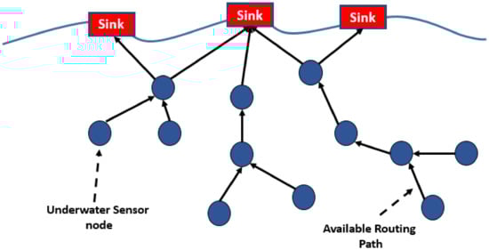
Figure 1.
Commonly used network architecture.
In this work we propose a suitable network architecture and a routing scheme that can handle partitioning in mobile UWSNs and thereby improve network performance by delivering higher volumes of traffic to the sink node. Our scheme consists of two phases. In phase 1, neighborhood information is disseminated in the network using beacons. In this phase, we propose a partition resolution strategy to reach and disseminate neighborhood information to the disconnected parts of the network. In phase 2, the neighborhood information collected in phase 1 is used to select appropriate relay nodes for forwarding the collected data to the sink node. A minimum residual energy threshold policy is used to enable busier nodes avoid early death in order to continue their sensing job. We also devise a rerouting strategy to route traffic in case a relay node cannot continue to operate as relay upon reaching its residual energy threshold.
In this work, we assume that all sensor nodes are freely mobile with underwater currents. All the sensor nodes transmit with same default transmission power initially. However, the transmission power can be increased when required. We assume that the relative positions of nodes do not change considerably in the short run. This assumption is reasonable because all the sensor nodes move within the same underwater stream. All nodes employ the multipath compensation strategy proposed in [13] to compensate for the multipath effect. Depth levels can be adjusted using pressure sensors; however, we deploy nodes at equal depth, thus forming a two-dimensional (2D) topology. Nevertheless, if we deploy nodes at different depth levels, the three-dimensional problem can be translated to 2D using depth information from pressure sensors.
Main contributions of this work are as follows:
- Network architecture is proposed that is suitable for mobile UWSNs.
- A partition resolution strategy is devised which improves network performance by improving the packet delivery ratio.
- A minimum residual energy threshold is used in order to delay early death of nodes and to shift the traffic load to the less loaded downstream nodes.
- In order to deal with connectivity holes, a loop-free re-routing scheme is devised to keep the network connected.
2. Literature Review
In [14], the authors propose a three-stage routing protocol aiming at tackling the energy hole minimization problem. In stage 1, nodes are deployed in circular regions around a sink node termed corona. Each corona region has equal width and the nodes deployed in a particular corona are equidistant from the sink node. In stage 2, load weights are calculated for every corona. Transmission ranges of nodes in a particular corona correspond to the load weight of that corona. This helps in achieving balanced energy dissipation. Stage 3 executes actual data transfer based on the predetermined topological setting and load weights. This scheme successfully reduces energy holes in the coronas near the sink node for fixed networks with predetermined topologies. However, in case of mobile networks where topology cannot be predetermined, the performance of this scheme may be seriously compromised.
In [15], the authors propose a cluster based routing protocol. Nodes are deployed in layers in such a way that the layers nearer to the sink nodes have smaller widths compared to the farther layers. The aim of this layering structure is to reduce the chances of creating hot spots by adjusting the transmission powers of nodes based on their distance from the sink node. Furthermore, nodes are grouped into clusters within each layer. Clusterhead for each cluster is selected based on its neighborhood connectivity, residual energy and its distance from the sink node. Data transmission begins once the clusters are formed. Relay selection is based on residual energy and distance of the candidate relay from the sink node. This scheme reduces chances of the early death of nodes due to energy drainage by reducing contention. The reduction in contention is achieved by setting contending radii of clusterheads according to their distance from sink.
In [16], the authors propose a cluster-based protocol for data collection. Nodes are positioned in hexagonal style and are grouped into a cluster. Cluster heads are selected based on the position of the nodes within the cluster and their residual energy levels. That is, the nodes that are located near the center of the cluster and have highest residual energy are the best candidate for selection as cluster heads. For data collection, [17] uses an Autonomous Underwater Vehicle (AUV) that uses ant colony optimization to determine shortest paths for its traversal in order to reduce end-to-end delays. The proposed scheme reduces end-to-end delays, and improves network lifetime through better energy management.
In [17], the authors propose a two-stage, depth-based routing scheme. In phase 1, called the update phase, nodes share information such as residual energy, node type, etc., with their neighboring nodes. This helps populate neighborhood tables of the nodes which are used to make forwarding decisions during the second phase, i.e., the routing phase. In the routing phase, void regions are avoided by proactive identification of such areas. As the process is carried out locally, it does not incur extensive communication overhead. The packet delivery ratio is improved by regulating the forwarding area according to the node density of the area ahead.
In [18], the authors propose a two-stage, multi-sink routing scheme. In stage 1, called the layering stage, nodes are deployed in concentric layered structure around each sink node thus forming a structure in which a particular node may be located in the layered structure of more than one node. The layers are refreshed if the packet delivery ratio (PDR) drops below a certain PDR threshold value. The layering stage is followed by the communication stage which selects an appropriate sink node for each node and also establishes and efficient path towards that sink. The criteria for route establishment aims at improving PDR and energy efficiency. The shortcoming of this protocol is the lack of mechanisms to handle connectivity holes.
In [19], the authors propose a Radius-based Multipath Courier Node (RMCN) routing scheme, a routing protocol for long-term sensing applications. The network is divided into two areas: the node area which takes ¾ of the total area and the sink area which constitutes ¼ of the total network area. The node area hosts equal numbers of static and mobile courier nodes whereas the sink area hosts sink nodes. Forwarders selection is based on the depth of the candidate node, its residual energy level its track ID and the outcome of a cost function. RMCN improves the PDR by well-organized coordination between static and mobile courier nodes, whereas energy consumption is controlled by avoiding flooding. However, as nodes are deployed according to a predefined criterion, RMCN may fail to perform in case of random deployment of nodes which is inherent in certain applications such as the cases where free mobility of nodes is considered.
In [20], the authors propose a cross-layer routing scheme that includes information from physical, Medium Access and network layers to make forwarding decisions. It is a two-hop forwarding solution in which forwarding decisions are made keeping in view the status of nodes up to two hops away from the sender. The sender selects a one hop forwarder, a relay node and a two-hop forwarder. A relay node is used for reliability. The protocol works in three stages. In stage one, neighborhood information is disseminated in the network. Stage two is related to route selection, whereas stage three deals with the transmission of actual data. This scheme improves reliability and thus improves PDR by incorporating cooperative routing in the form of redundant relay nodes besides the actual forwarder. However, this redundant transmission every two hops increases communication overhead and contention, which consequently increases energy consumption.
In [21], the authors propose a joint design of Power Control and opportunistic Routing (PCR). The proposed scheme aims at improving PDR. It carries out its operations in three stages: In Stage one, neighborhood information in the form of beacons is transmitted by every node using all available power levels. In stage two, candidate forwarders are selected based on the information received during phase one. This phase takes into account every possible power level and selects one forwarder corresponding to each of the available power levels. Energy consumption is considered in order to improve energy efficiency. Stage three deals with the transmission of data and coordination among forwarders in such a way that energy dissipation is balanced. As in PCR, beacons are transmitted using all available power levels, and hence multiple transmission of the same information creates a huge communication overhead which in turn increases the contention and energy consumption. This will lead to creation of connectivity holes and partitions in the network and, consequently, a low packet delivery ratio. Moreover, in the case of mobile network, stage one should be carried out periodically, thus increasing the energy consumption many-fold.
Besides the above, many other routing schemes have been proposed. For instance, [22] is a cluster based Quality of Service aware routing protocol that deploys nodes in a hierarchical order to achieve balanced distribution of traffic and energy dissipation. Route establishment and forwarding are carried out in a greedy manner based on the link quality between clusterheads. Moreover, transmission range variation is used to deal with failed nodes and connectivity holes. In [23], the authors propose three routing schemes that work in collaboration to achieve high energy efficiency and fair load distribution. Transmission power is altered according to the energy level of the forwarder, traffic load and distance between the forwarder and the sender. It attains balanced distribution of traffic load by taking into account residual energy while selecting a forwarder. In [24], a reactive source routing scheme is proposed. The use of source routing enables the source node to determine the whole path from itself to the destination. The scheme takes cross-layer approach by a Stop-and-Wait Automatic Repeat Request (ARQ) which enables it to identify overloaded links and unpredictable routes.
All the above-mentioned protocols assume limitedly mobile or static sensor nodes. Therefore, when faced with mobility induced issues such as network partitioning, the performance of the protocols may suffer setbacks. Moreover, many of these protocols deploy nodes according to predetermined deployment patterns and then design the protocol accordingly. If the topology changes, for instance due to mobility, the performance of such protocol may go down.
3. Methodology
The proposed scheme consists of two phases: the neighborhood information acquisition phase, and the relay selection and transmission phases. During the neighborhood information acquisition phase, nodes transmit beacons to share their residual energy and hop count information. Those nodes which do not receive a beacon until a predefined threshold time, request beacon by transmitting beacon requests. In the relay selection and transmission phase, upon reception of data, nodes select the best next hop node to forward the received data towards the sink node. The next hop node is selected based on link condition, residual energy and hop count.
3.1. Network Model
Figure 2 illustrates our network model. The network consists of n sensor nodes, one underwater sink node (UW-Sink), m backup UW-Sink nodes and one surface sink node. All the underwater nodes move freely within the same underwater stream. The sensor nodes send the sensed data to the UW-Sink periodically. The UW-Sink is connected to the surface sink node using a long-haul connection which is used to transfer the data collected from the underwater sensor node to the surface sink node. We assume that the UW-Sink nodes have abundant energy resources for long-haul communication. The backup UW-Sink nodes, which also act as ordinary sensor nodes, take the role of UW-Sink in case of failure of the main UW-Sink. Every UW-Sink is equipped with movement tracking apparatus using which it can estimate its distance from its initial position at the time of deployment and thus, its distance from the surface sink node at any given time. This distance information is necessary for range adjustment, as the nodes move away from initial deployment position.
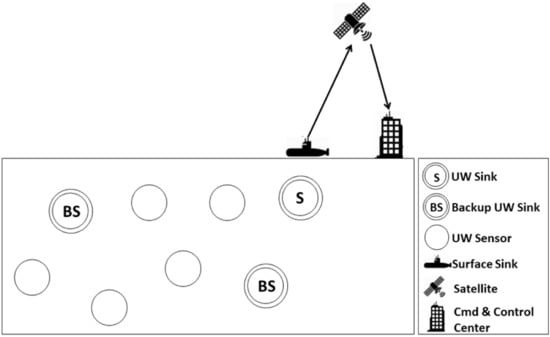
Figure 2.
Network model.
Transfer of Control among UW-Sink nodes: The transfer of control may be required if the energy level of the active UW-Sink node reaches a certain threshold. In such a case, the UW-Sink node exclusively instructs one of the backup UW-Sink nodes to take control from the next iteration. This can be done in many ways. For instance, the backup node can be informed through a special bit piggy-backed in a routine beacon. The message can be protected using forward error correction (FEC). As the number of control transfers is normally negligible, addition of FEC bits to a “transfer of control” message has a very insignificant effect on the protocol performance. Other options, such as sending a message on an exclusive control channel or sending a “transfer of control notification” on the same channel either through multihop communication or directly with increased range, also exist.
3.2. Underwater Channel Model
The behavior of the underwater channel is influenced by many factors such as signal attenuation, noise and the speed of sound in the underwater medium which are described as follows:
Transmission Loss: Transmission loss is the drop in the intensity of the transmitted signal as it travels the medium from the sender to the receiver. Transmission loss has two major constituent factors; absorption loss and spreading loss. Equation (1) [25] represents transmission loss in an underwater acoustic channel over distance l and frequency f.
where k is the spreading factor and the α(f) stands for absorption coefficient. Commonly used values of k are 1.5 for practical spreading, 2 for spherical spreading and 1 for cylindrical spreading where α(f) can be computed using Equation (4).
Attenuation: The power of a transmitted signal in the underwater acoustic channel reduces as it travels from source to destination. Major factors contributing to the attenuation of a transmitted signal in the underwater acoustic channel are distance, frequency spreading of the acoustic waves and absorption. Attenuation over a distance l using frequency f in an underwater acoustic channel can be estimated using Equation (2) [26],
where l, α, f, c and Ao represent distance, absorption coefficient, frequency, spreading factor and normalization constant, respectively. The attenuation can be denoted as in decibel (dB) using Equation (3) [26].
The absorption coefficient α is represented by Thorps model (Equation (4)) [26].
Equation (4) is used for frequencies above a few hundred Hertz. However, Equation (5) [26] is used for smaller frequencies.
Speed of Sound: The speed of sound underwater may vary between 1450 m/s to 1550 m/s based on temperature, depth and salinity of water [26]. In [27], the authors modeled an empirical equation for the speed of sound in water given as Equation (6) below:
where c, T, S and D represent the speed of sound in water, temperature in Celsius scale (°C), salinity in parts per thousand and depth in meters, respectively.
Channel Noise: The ambient noise in the underwater environment has four major contributing factors which are shipping activity, breaking waves, turbulence and thermal noise [28]. Equations (7)–(10) [28] represent the PDFs of noises due to shipping activity, waves, turbulence and thermal noise, respectively.
3.3. The Routing Process
Our routing procedure is performed periodically every N units of time. Every instance of the routing procedure is termed as routing cycle. Every routing cycle has two major constituent phases: The Neighborhood information acquisition phase, in which beacons are used to disseminate neighborhood information; and the relay selection and data transmission phase, during which the data collected by the sensor nodes is delivered to the UW-Sink through relay nodes. Each sensor node selects its next hop/Relay node based on the information collected during the Neighborhood information acquisition phase. Before we explain the routing phases in detail, we explain the network scenarios that our protocol addresses.
3.3.1. Network Partitioning Scenarios
We identify two types of network partitioning.
Scenario 1:Figure 3 shows network partitioning scenario 1. Network partitioning occurs when one or more nodes drift apart from the main body of the network due to mobility and therefore are not able to receive beacons. Here, the main body of the network refers to those nodes that can receive beacon directly or indirectly (through two or more hops) from the UW-Sink. All those nodes which have not received a beacon do not have neighborhood information. Due to the fact that a partitioned node cannot reach the main body of the network with default range, absence of neighborhood information results in the inability of such nodes to send their data.
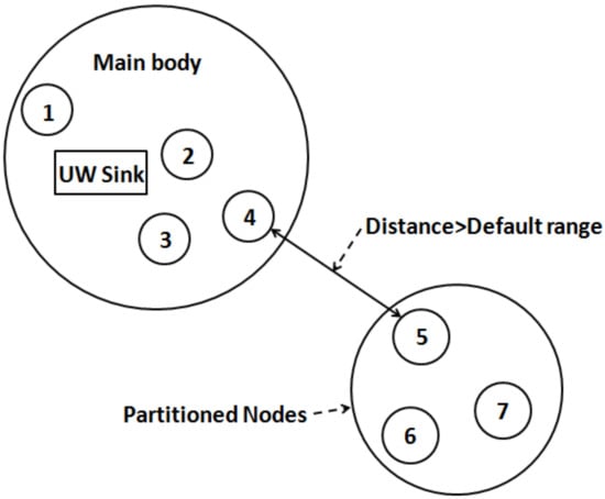
Figure 3.
Network partitioning due to mobility.
Scenario 2:Figure 4 shows network partitioning scenario two which occurs when nodes in an otherwise connected network die out due to energy drainage. In such a case, all those nodes whose route to the UW-Sink passes through a dead node get partitioned and are not able to send data to the UW-Sink.
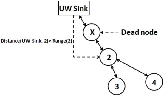
Figure 4.
Network partitioning due to connectivity holes.
It is important to note that scenario 1 occurs before the neighborhood information acquisition phase, whereas scenario two occurs during the data forwarding after the neighborhood dissemination phase.
3.3.2. Neighborhood Information Acquisition Phase
The neighborhood information acquisition phase uses the ALOHA protocol for channel access. This phase can be subdivided into two steps. In step 1, the UW-Sink initiates the neighborhood information acquisition phase by transmitting a beacon with transmission power p. Each sensor node that is located within the communication range of the UW-Sink receives the beacon and sets its minimum hop count to the sink node to one. After the reception of the first beacon, the receiving nodes set up a waiting time Wt during which they wait for the arrival of beacons from other nodes. This is done to gather further neighborhood information. Acquiring information from more than one neighbor offers flexibility and reliability in case of failure of a next hop neighbor (further explained in Section 3.3.3). At the end of the Wt of a node, the node creates a beacon containing its residual energy information and minimum hop count along with the neighborhood information received from the neighboring nodes. The minimum hop count for any receiver X is one plus the minimum hop count of the node whose minimum hop count is minimum among all the neighbors of node X. The updated beacon is retransmitted using the default transmission power. All the nodes further down the stream update their hop count based on the received beacons and repeat the above mentioned process upon reception of beacons. Consequently, every single and multihop neighbor X of the sink node has the following information:
- (1)
- One and two hop neighbors of node X. We refer to the set of one hop neighbors of node X as Nx and the set of two hop neighbors of node X as N2x
- (2)
- Minimum hop count of all the nodes in sets Nx and N2x
- (3)
- Residual energies of all the nodes in sets Nx and N2x
- (4)
- Distance of every node in Nx from node X and distance of every node in N2x from their corresponding node in Nx (i.e., the node in Nx that received beacon from the node in N2x).
During step 1, the single and multiple hop neighbors of the UW-Sink receive beacons. Single and multihop neighbors refer to those nodes that can be accessed over single or multiple hops, while the default transmission power is being used by all the nodes. However, the partitioned nodes that are out of the default communication range of the UW-Sink and all the beacon carrying nodes will not receive beacon during step 1 of the neighborhood information acquisition phase. These partitioned nodes initiate step 2 proactively by sending beacon requests after a certain threshold time TR with increased transmission power. As all the nodes have the same initial transmission power, lack of reception of a beacon stresses the need for increased transmission power for sending requests in order to increase the chances of finding a beacon hosting node in the neighborhood. After transmission of the beacon request, the requesting node goes into wait state for time Tw which is given as
where Tpr represents the processing delay, R is the current range, and C denotes the speed of sound under water. The second term, α, is used to compensate for channel asymmetry. We note that R/C measures the maximum propagation delay.
Tw = 2 R/C + α + Tpr
Any beacon hosting node that receives a beacon request responds by transmitting beacon with transmission power equal to that of the sender of the beacon request plus an offset value that is used to compensate for the lack of symmetry in the underwater channel. This ensures that the transmitted beacon reaches the requesting node. However, there are two possible failure scenarios:
- A partitioned node may not find a beacon hosting node even with increased transmission power as the beacon hosting nodes may be farther away.
- The beacon transmission in response to a request is lost due to collision or channel impairments.
If a requesting node does not receive beacon within its Tw due to either of the above-mentioned failure scenarios, it resends beacon request by further increasing its transmission power and also sets Tw using (1). The number of attempts can be pre-determined based on the deployment pattern and the characteristics of the underwater stream carrying the sensor nodes.
Link Budget: In order to deal with the high bit error rate of the underwater channel, the next hop selection criteria (explained in Section 3.3.3) includes link condition. Link budget is used to estimate the received power level of a signal at destination D located x meters from the source where the signal is transmitted over frequency f.
Upon reception of a beacon, the receiver R estimates its distance from the sender S using the distance and frequency information along with other channel parameters; R estimates the achievable power level at S. It is important note that the beacon receiver R will potentially send data to the sender S in the data transmission phase. Therefore, it calculates the link budget (i.e., the estimated received power level at S) for its potential data transmission to S. The link budget information is added to the neighborhood table of R to be used during relay selection process.
If the expected received power is within the acceptable limits, i.e., Eo/No, the node in question is selected for further evaluation as next hop, i.e., hop count and Residual energy evaluation (details in Section 3.3.3).
Equation (13) [29] represents the link budget for the underwater wireless channel
where SNR, PL, TL, N, and represent Signal to noise ratio at destination (received power), Pressure Level at the transmitter (transmitted power), transmission loss, ambient noise, directivity index of the sender and the directivity index of the receiver, respectively. All the above quantities are stated in dB re 1 µPa. As we are assume use of omni directional antenna and are set to zero. Figure 5 shows a block diagram of the link budget as expressed in Equation (13).
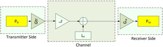
Figure 5.
Block diagram of the link budget [26].
The signal power at the receiver can be converted to electrical power using
Required signal Level (Eo/No): The required signal level which is a function of the desired bit error rate can be defined as the ratio of energy per bit to receiver noise level, i.e., Eo/No [29].
Available signal Level: The product of the link budget analysis is available SNR at the receiver. To compare with required, received power is translated to an energy-per-bit equivalent using Equation (16) [29].
where , , , B and D represent, received power (SNR), energy required per bit of information, receiver noise in 1 Hz of bandwidth, spectral bandwidth and data rate, respectively.
The link margin (LM) compares received power level with that required for the established BER (Equation (17)) [29]
Based on the above-mentioned comparison, i.e., the link margin reception is considered a success or failure.
In Figure 6, we show a flowchart that illustrates the neighborhood information acquisition phase.
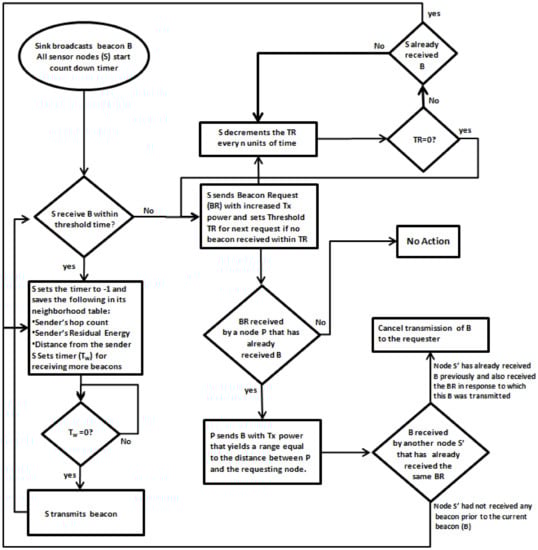
Figure 6.
Neighborhood information acquisition phase.
3.3.3. Relay Selection and Data Transmission Phase
Relay Selection
This phase deals with hop by hop transmission of data from source node to the UW-Sink. Every node, that has a data packet to send (either of its own or received from a downstream node) searches in its neighborhood table for the nodes which have acceptable link condition (received power), minimum hop count to the UW-Sink and maximum residual energy. The neighborhood table contains IDs of the neighboring nodes y, the total hop count to the UW-Sink through any particular node y, the residual energy of node y, the expected received power at node y and the distance between node x (neighborhood table host) and that particular node y. The table is sorted in ascending order of hop count subject to link condition, i.e., if the expected received power at the destination node x is above a certain threshold and it is the minimum hop count node, node x goes top of the list. The topmost node is used as the next hop relay. However, if there are more than one nodes that fulfill the above-mentioned criteria, residual energy becomes the deciding factor. That is, the node with highest residual energy among the least hop count nodes is selected as relay. This helps in delaying connectivity hole creation and in achieving low end-to-end delay. It is important to note that a node with estimated received power below the required threshold will not be considered as the relay irrespective of its hop count and residual energy. Figure 7 elaborates upon the relay selection process.
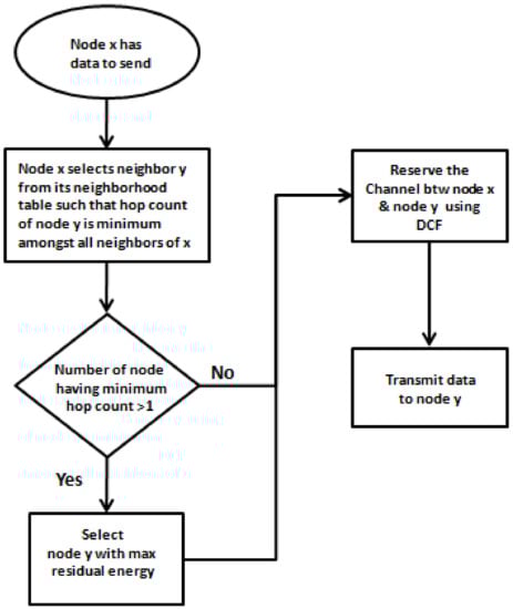
Figure 7.
Relay Selection.
Data Transmission
During this phase, all the nodes that have data send their packet to their next hop nodes. We use the Distributed Coordination Function (DCF) to deal with the contention related issues. (Besides providing a solution to the hidden node problem, DCF also helps in dealing with the harsh underwater environment through the ACK mechanism. The ACK function in the DCF ensures that packet delivery to the next hop is confirmed. If ACK is not received the packet is resent). Every node that has a data packet to send forwards the packet to its predetermined next hop by reserving the channel through RTS/CTS exchange. A successful reception at the destination is acknowledged with an ACK frame from the receiver. As every node takes the shortest possible path, certain nodes with higher traffic volume may drain their energy early. Consequently, such sensor nodes die out early during the sensing mission, thus reducing the number of sensor nodes deployed for the sensing mission. To deal with this problem, we propose that every node maintains a minimum residual energy threshold. Upon reaching the threshold, the node refuses to act as relay for other nodes. In response, the neighboring nodes, whose next hop is a node that refused to act as relay node, reroute their traffic through other neighboring nodes. The process is explained as follows.
Rerouting
Whenever a node’s residual energy level reaches the minimum residual energy threshold, it transmits a notification to inform all its neighbors about itself quitting the forwarder/relay role. The notification also contains a list of neighbors of the quitting node. Upon reception of the notification, the neighboring nodes reorient their neighborhood tables by removing the quitting node from their neighborhood tables. The topmost node in the reoriented table (that represents the least hop count node with acceptable level of expected received power) is selected as the relay node. If more than one node have the minimum hop count to the UW-Sink, the node with maximum residual energy is selected as relay. However, there is possibility that:
- All the one hop neighbors have reached their minimum residual energy threshold.
- There is no other one-hop neighbor in the list.
In the first case, any node X, whose predetermined next hop node is a quitting node, searches for a suitable next hop node in the one-hop neighbors of its neighbors. If a suitable next hop node is found in the neighborhood of a neighboring node Y, node X increases its range equal to its distance from node Y plus node Y’s distance from the neighbor which is being considered as next hop.
In the second case, i.e., when there is no other neighbor except the current next hop node (i.e., the quitting node), node X searches for a suitable next hop node in the one hop neighborhood of its current next hop node.
However, if no appropriate next hop node is found even in the neighborhood of the neighboring nodes, the packet for this cycle is dropped. Our partition handling mechanism ensures that the node finds an appropriate next hop node in the next Cycle. Rerouting can be explained using Figure 8.
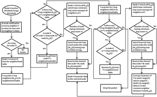
Figure 8.
Relay selection and rerouting.
Forwarding Loop
Consider the scenario in Figure 8. In this figure, we assume that node one has two available routes (one through node 2 and the other through node 4) to send its data to the UW-Sink. However, node 2 offers the least hop count to the UW-Sink. Therefore, node 2 is selected as relay for node 1. Node 2 has only two nodes in its neighborhood, i.e., node 1 and node 3. Node 3 is relay for node 2 as it offers smaller hop count as compared to node 1. In order to understand loop creation, we assume that node 3 reaches residual energy threshold and therefore it denies relay service to node 2. In response, node 2 selects node 1 as its next hop as there is no other node in node 2’s neighborhood table (node 4, 5 and 6 are out of node 2’s current communication range). This will create a loop where node 1 and node 2 keep forwarding data to each other, thus, are not able to deliver data to the UW-Sink.
Forwarding Loop Resolution
If at any time a node X receive a data packet from another node Y where Y is the next hop node of node X, node X changes its next hop. For changing the next hop, node X removes node Y from its neighborhood table and selects the least hop count neighbor from the remaining nodes. For instance, in Figure 9, upon reception of an RTS packet from node 2 (which is node 1’s next hop node), node 1 removes node 2 from its neighborhood table and evaluates the remaining nodes in its table to select the best forwarder, i.e., node 4. This will result in breaking the loop and avoiding connectivity loss due to loops.
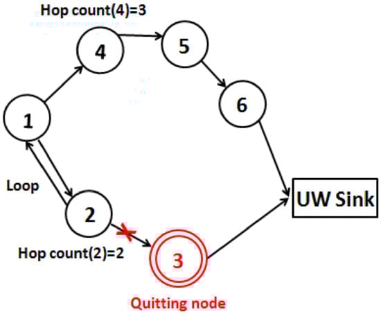
Figure 9.
Forwarding Loop.
Why Residual Energy Threshold
Connectivity holes are created because the nodes nearer to the UW-Sink have a higher volume of traffic going through them. This results in early drainage of their batteries thus disabling the nodes, which are sending data through them to reach the UW-Sink. According to [8], when the nodes near the UW-Sink have consumed all their initial energy deposit, the nodes farther down the stream have 93% of their energy deposit intact. Thus, if the connectivity holes are not resolved, even though the farther nodes have enough energy, it is not useful as the packets from such node may not be delivered. Moreover, the relay nodes are also sensor nodes. Therefore, the early death of a relay node reduces the number of nodes assigned for the underwater sensing mission. The residual energy threshold ensures delay in the early death of sensor nodes. Secondly, our partition handling mechanism ensures that the load is shifted down the network to the less loaded nodes thus ensuring better distribution of energy consumption across the network.
This can be explained with the help of the Figure 10:
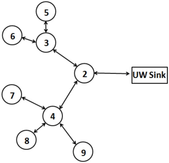
Figure 10.
Rationale for Residual Energy Threshold.
In this example, we assume that only node 2 is directly connected to the UW-Sink. Nodes 3 and 4 are within the range of node 2, which enables them to receive beacon from node 2. Whereas, nodes 5, 6 and nodes 7, 8 and 9 fall within the communication range of nodes 3 and 4, respectively. For the sake of simplicity, we assume that none of the above-mentioned nodes fall within the communication range of any other node except for those mentioned above.
As evident from the topology, the traffic load is highest on node 2, followed by nodes 4 and 3, whereas nodes 5 to 9 have the smallest load which is their own data packets. Intuitively, we can tell that node 2 will reach its residual energy threshold before other nodes. If node 2 keeps forwarding data from this point onwards, it will soon run out of energy and will not be able to continue its role a sensor node. However, if node 2 quits forwarding, a connectivity hole will be created. In the absence of other neighboring nodes, the rest of the network will not be able to reach the UW-Sink, thus bringing down the packet delivery ratio to zero. For the ongoing routing cycle, this issue is resolved by our rerouting mechanism which ensures that the load is shifted down the network to the less loaded nodes, i.e., nodes 3 and 4. Moreover, in the following routing cycles, our partition handling routine solves the issue amicably by shifting the load backwards. In the next routing cycle, node 2 will not send beacon thus none of the neighbors will be able to route traffic through node 2. After the threshold time, the remaining nodes will send requests with increased transmission power. We assume that nodes 3 and 4, being nearer to the UW-Sink, receive a beacon from the UW-Sink which they retransmit. The beacons are received by their neighbors, i.e., nodes 5 to 9. Now nodes 3 and 4 will directly transmit data from nodes 5,6,7,8 and 9 to the UW-Sink. The same process will be followed when nodes 3 and 4 reach their residual energy threshold. This technique effectively distributes energy consumption across the network. Even though farther nodes have to use higher transmission power to send their data that results in higher energy consumption, this technique keeps the network connected. The high residual energy in the downstream network nodes may be wasted if the network disconnects due to connectivity holes.
3.4. Protocol 1.1: No Partition Handling (NPH)
We define Protocol 1.1, a generic routing protocol for underwater acoustic sensor networks. It works in two stages: Beacon dissemination and data transmission stages. During the beacon dissemination stage, the sink node initiates the process by transmitting a beacon which is then forwarded by every node that receives the beacon. Based on the neighborhood information acquired during the beacon dissemination stage, every node determines its next hop node. The next hop selection criteria is based hop count and residual energy. Protocol 1.1 differs from the proposed protocol in the following respects:
- Unlike the proposed protocol, protocol 1.1 does not incorporate any partition handling mechanism. Therefore, in case of network partitioning, the partitioned part will not be able to receive beacons and therefore will not be able to access the main body of the network. The drop in the packet delivery ration will depend upon the number of partitioned nodes besides other factors such as connectivity hole and erroneous reception.
- Unlike the proposed protocol, protocol 1.1 does not implement any mechanism for diverting the traffic load to less burdened, high residual energy downstream nodes.
- Protocol 1.1 does not incorporate a loop resolution strategy.
- Protocol 1.1 does not enforce any minimum residual energy threshold and therefore does not follow the actions taken by the proposed scheme when a node reaches its residual energy threshold.
Protocol 1.1 has the following similarities with the proposed scheme:
- Protocol 1.1 assumes untethered free mobility of sensor nodes with water currents. It, therefore, assumes the same network architecture as that of the proposed scheme.
- Next hop selection criteria is the similar to that of the proposed scheme. The candidate nodes are first evaluated based on the link condition. The nodes with acceptable expected SNR are shortlisted. Among the shortlisted nodes, the nodes with minimum hop count and maximum residual energy are selected as next hop.
The reason for comparing our scheme with protocol 1.1 is lack of available protocols that follow similar network architecture and/or assume free untethered mobility of sensor nodes. To the best of our knowledge, this area still remains to be explored.
4. Results and Discussion
Based on the operation of the proposed protocol, our protocol needs functionality only up to data link layer level. On the link level, for channel access we use the ALOHA protocol for dissemination of beacons and requests and DCF for data forwarding. Through our channel model, we acquire the required physical parameters for our work. We used Matlab R2016b to simulate our protocol. Table 1 shows simulation parameters.

Table 1.
Simulation Parameters.
In all the following results, PH refers to the proposed scheme whereas No-PH refers to protocol 1.1. The results are averaged over 50 random topologies for all the different number of nodes.
4.1. Network without Partitions
This section shows results for networks that are not partitioned at the start of a routing cycle. However partitions may or may not occur in later routing cycles due to dying nodes.
4.1.1. Number of Delivered Packets
Every node has exactly one data packet to send per routing cycle.
Figure 11 shows the percentage of the number of successfully delivered packets for networks consisting of 25, 50, 75 and 100 nodes. The considered networks do not have any partition initially. However, connectivity holes may be created that may or may not result in network partitioning. Our proposed scheme shows improvement in the number of delivered packets. The improvement is achieved due to our residual energy threshold policy. When a node reaches its residual energy threshold, it denies relay service to downstream nodes. This helps maintain the number of delivered packets as the data traffic is taken off the nodes with low energy and routed through high energy nodes. This enables the low energy nodes stay alive longer to send only their own data packet. (It is important to note that, besides other factors such as connectivity holes, collisions, etc., the number of delivered packets reduce with number of dying nodes as every node sends one data packet per routing cycle. Therefore, if one node dies, we have one less packet in the total number of delivered packets). Moreover, in case of denial of relay service, our rerouting mechanism extends the forwarder search area to the two-hop neighborhood, thus increasing the chances of a successful packet delivery. Furthermore, if one or more nodes cannot find any next hop node even in its two-hop neighborhood, our partition handling routine will connect it in the next routing cycle, thus maintaining a higher packet delivery ratio. Compared to PH, in NPH nodes nearer to the UW-Sink die out earlier as NPH does not follow any residual energy threshold policy. The death of nodes may result in the creation of connectivity holes which, in the absence of rerouting mechanism, results in a lower number of delivered packets.
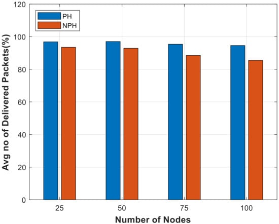
Figure 11.
Number of delivered packets.
The number of delivered packets for PH is highest for 25 nodes; however, it drops slightly due to increased contention as the number of nodes increase. Similar trend can be observed in case of NPH.
4.1.2. Death Ratio
Figure 12a–d show the number of dead nodes for 25, 50, 75 and 100 nodes, respectively, over the routing cycles intervals of 1–20, 21–40 and 41–50. In all four cases, PH shows a smaller number of dead nodes in each interval. This is due to the residual energy threshold policy which prevents early death of nodes by allowing highly burdened nodes to deny relay service upon reaching their residual energy threshold and by rerouting traffic through other nodes having enough residual energy. (It is important to note that the last interval is only 10 routing cycles as compared to 20 routing cycles in the first two intervals. Therefore, our graphs show smaller number of dead nodes in the last interval). The number of dead nodes increases with increasing routing cycles as nodes run out of their energy due to transmission (mostly relay transmissions) in previous routing cycles. Overall, the number of dead nodes in each interval increases with the increasing number of nodes. The reason for the increase is that higher number of nodes increases load on the nodes nearer to the sink node. However, the rise is not too high due to the following two reasons. Firstly, a higher number of nodes inherently distributes load by offering multiple relay options. Secondly, our link condition criteria for selecting the next hop node improves successful reception of packets which consequently reduces unnecessary transmissions and energy consumption.
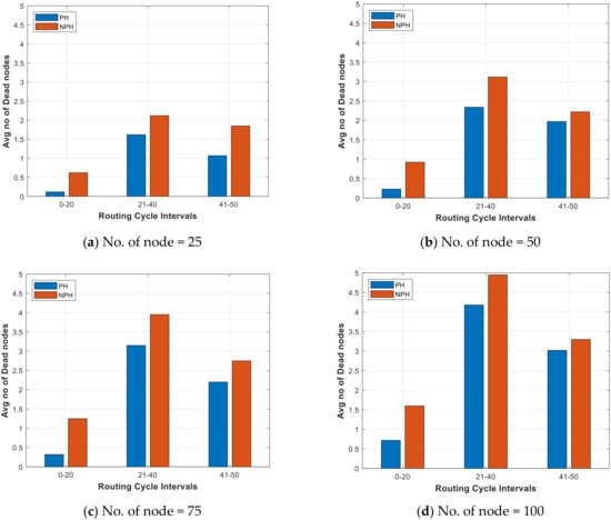
Figure 12.
Death Rate. Descriptions for (a–d) are given in figure.
4.1.3. Communication Overhead
Figure 13 shows the communication overheads of PH and NPH. PH has slightly higher communication overhead due to the following two reasons:
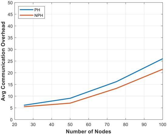
Figure 13.
Communication Overhead.
- In case of partitioning in the network, PH involves transmission of localization requests. Beacons are transmitted in response to the requests by the nodes that receive the request. However, if a particular node that received a request and subsequently heard a beacon destined for the requester it abandons transmission of the beacon.
- Unlike NPH, in PH when a node reaches its residual energy threshold it transmits a notification to inform its neighbor about denial of relay service, thus adding to the overall communication overhead.
As the number of nodes increase from 25 to 100, the gap between the two curves increases. The reason for this is again the higher communication overhead in the form of relay service denial notifications and request and subsequent beacons due to connectivity holes. With increase in the number of nodes, this overhead (which is specific to PH only) increases, thus widening the gap between the two curves.
4.1.4. Energy Consumption
We assume that all nodes are equipped with Evo Logic’s S2CR 48/47 acoustic modem [30].
Figure 14 shows the overall average energy consumption. The higher communication overhead, in the form of “denial of relay service” notifications, localization requests and corresponding beacons in case of partition, results in higher energy consumption. Another very important reason for the gap between the energy consumption of the two schemes is absence of transmission activity by the partitioned nodes due to the lack of partition handling capability in case of NPH. As there is no partition handling mechanism in NPH, if a node gets partitioned, it will not be able to receive any beacon and, thus, will not indulge in any transmission activity. This will keep its energy intact thus widening the gap between the two curves. Moreover, the elimination of partitioned nodes also reduces contention (and therefore reduces energy consumption) in the main body of the network as fewer nodes contend for the medium. However, being unable to connect the partitioned nodes, NPH achieves lower packet delivery ratio. As partitioned nodes cannot send their sensed data, it results in a reduction of the number of deployed nodes for the sensing mission. The disconnected nodes are useless as their data cannot be delivered.
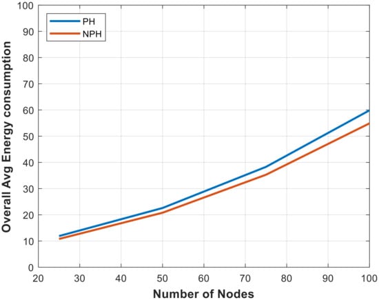
Figure 14.
Energy Consumption.
4.2. Partitioned Network
This section shows results for partitioned network. In order to focus only on the partition handling ability (which is clearly indicated by the number of delivered packets), we keep the initial energy level to 300 joules.
4.2.1. Packet Delivery Ratio
Figure 15 shows the number of delivered packet by PH and NPH for 25, 50, 75 and 100 nodes. The proposed scheme (PH) achieves higher packet delivery ratio in all the cases. The reason for the better performance is the partition handling mechanism which allows the partitioned nodes, which cannot receive a beacon because of being out of the range of all the beacon-carrying nodes, to request beacon with increased transmission power. Secondly, nodes stay alive longer in case of PH due to the residual energy threshold policy. As the number of delivered packet is just count, an alive node adds to it if its packet is delivered. However, if a node dies, the count goes down by one as a dead node cannot send data. On the other hand, in case of No-PH, a partition handling mechanism does not exist. Therefore, in case of No-PH, partitioned nodes cannot receive a beacon and, as a result, cannot send their packets thus cutting down the number of packets by at least the number of partitioned nodes. A further reduction in the number of delivered packets is caused by connectivity holes and early death of nodes with higher loads.
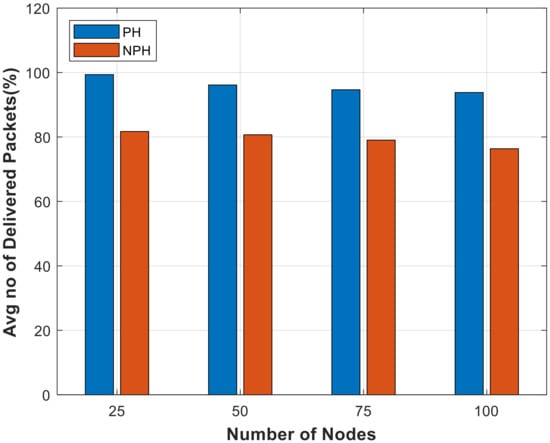
Figure 15.
No. of delivered packets (Partitioned Network).
4.2.2. Death Rate
Figure 16a–d show the number of dead nodes for 25, 50, 75 and 100 nodes, respectively, over the routing cycles intervals of 1–20, 21–40 and 41–50. For 25 and 50 nodes, PH shows a smaller number of dead nodes compared to NPH. Comparison of the death rate figures of the partitioned networks with those of unpartitioned networks reveals that the difference between the death rates of PH and NPH is reduced, i.e., the death rate of PH has increased whereas the death rate of NPH has reduced in the case of partitioned networks. The increase in the death rate of PH is caused due to the additional transmissions (in case of partitioned networks) in the form for localization requests and the corresponding beacons plus additional contention due to the transmission of these packets. Due to the same reason, the number of dead nodes in the 2nd and 3rd interval in the case of 75 and 100 nodes goes higher in PH as compared to NPH. The increase in the requests, response beacons and higher contention created due to bigger number of nodes, increases energy consumption and thus increases the no. of dead nodes. How can PH still produce better packet delivery ration despite its slightly higher death rate in case of 75 and 100 nodes. The answer lies in the functioning of NPH. In case of NPH, the nodes which get partitioned, do not have any mechanism to receive beacons. Therefore, despite having enough energy, these nodes can neither transmit their own data packets, nor can they act as relay. Therefore, their energy remains intact which results in a lower death rate. However, as the partitioned nodes cannot transmit their packets, the overall number of delivered packets is reduced at least by the number of partitioned nodes. On the other hand, PH incurs some additional cost, in the form of request and beacon response packet, in order to access the partitioned nodes thus enabling them to transmit their data, thereby improving the packet delivery ratio.
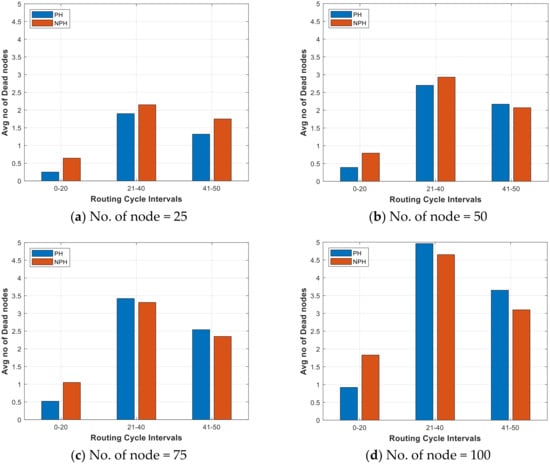
Figure 16.
Death Rate. Descriptions for (a–d) are given in figure.
In case of 25 nodes, PH has a lower number of dead nodes during routing cycle number 21 to 40 and 41 to 50, respectively. Due to the smaller number of nodes, the effect of traffic generated due to our partition handling mechanism is minimal. Thus, even though the proposed scheme improves the packet delivery ratio, the volume of overhead for partition handling is small and therefore does not affect the death rate considerably. Moreover, as explained before, the early death of nodes is avoided by the introduction of residual energy threshold.
In case of 50 nodes, a similar affect can be observed. However, the number of dead nodes in PH during the same intervals has increased compared to 25 nodes. Moreover, the difference between the number of dead nodes of PH and No-PH has also decreased. This is due to the increasing overhead of PH to carryout partition handling routine.
In PH, in case of 75 nodes, a higher number of partitioned nodes generates higher communication overhead in the form of localization requests and response beacons. Besides, overhead due to contention also increases, thus resulting in higher number of dead nodes in case of PH compared to NPH. The smaller number of dead nodes in case of NPH is also due to the fact that the partitioned nodes do not transmit at all, thus reducing the contention domain. With a smaller contention domain, fewer packets are lost which reduces death rate of NPH in the later routing cycles. However, this reduction in death rate is achieved at the cost of eliminating partitioned nodes and thus reducing the packet delivery ratio. PH, on the other hand, keeps the network connected by allowing the partitioned nodes to send some extra packets in the form of beacon request.
5. Conclusions
In this work, we proposed a two-stage routing protocol for mobile underwater sensor networks. We specifically focused on network partitioning problem. Partitions are resolved by allowing the partitioned nodes to access the main body of the network by sending beacon requests with increased transmission power. The beacon received in response enables the partitioned nodes to connect to the main body of the network. Besides, we also proposed a minimum residual energy threshold aiming at avoiding early death of burdened nodes and transferring the burden to the less busy nodes. Furthermore, a rerouting scheme based on two-hop neighborhood information is proposed to reroute traffic in case of connectivity holes. Overall, we improve the packet delivery ratio by enabling the partitioned nodes to send their data. Moreover, our minimum residual energy threshold scheme successfully delays complete energy drainage, thus allowing nodes to continue their sensing job for a longer period of time. In future research, we want to further enhance the functionality of the proposed scheme by using multiple simultaneously working, strategically deployed sink nodes. Moreover, we also plan to improve the partition handling mechanism by introducing clustering.
Author Contributions
Writing—original draft preparation, T.I.; writing—review and editing, S.-H.P. All authors have read and agree to the published version of the manuscript.
Funding
This work was supported by the Basic Science Research Program through the National Research Foundation of Korea (NRF) grants funded by the Ministry of Education under Grants NRF-2018R1D1A1B07040322 and NRF-2019R1A6A1A09031717.
Conflicts of Interest
The authors declare no conflict of interest.
References
- Luo, J.; Fan, L.; Wu, S.; Yan, X. Research on Localization Algorithms Based on Acoustic Communication for Underwater Sensor Networks. Sensors 2017, 18, 67. [Google Scholar] [CrossRef] [PubMed]
- Felemban, E.; Shaikh, F.K.; Qureshi, U.M.; Sheikh, A.A.; Qaisar, S. Underwater Sensor Network Applications: A Comprehensive Survey. Int. J. Distrib. Sens. Netw. 2015, 11, 896832. [Google Scholar] [CrossRef]
- Heidemann, J.; Ye, W.; Wills, J.; Syed, A.; Li, Y. Research challenges and applications for underwater sensor networking. In Proceedings of the WCNC 2006 IEEE Wireless Communications and Networking Conference, Las Vegas, NV, USA, 3–6 April 2006; Volume 1, pp. 228–235. [Google Scholar]
- Kumar, R.; Singh, N. A Survey on Data Aggregation and Clustering Schemes in Underwater Sensor Networks. Int. J. Grid Distrib. Comput. 2014, 7, 29–52. [Google Scholar] [CrossRef]
- Luo, J.; Fan, L. A Two-Phase Time Synchronization-Free Localization Algorithm for Underwater Sensor Networks. Sensors 2017, 17, 726. [Google Scholar] [CrossRef]
- Akyildiz, I.F.; Pompili, D.; Melodia, T. Underwater acoustic sensor networks: Research challenges. Ad Hoc Netw. 2005, 3, 257–279. [Google Scholar] [CrossRef]
- Islam, T.; Lee, Y.K. A Comprehensive Survey of Recent Routing Protocols for Underwater Acoustic Sensor Networks. Sensors 2019, 19, 4256. [Google Scholar] [CrossRef]
- Bouabdallah, F.; Zidi, C.; Boutaba, R. Joint Routing and Energy Management in UnderWater Acoustic Sensor Networks. IEEE Trans. Netw. Serv. Manag. 2017, 14, 456–471. [Google Scholar] [CrossRef]
- Jin, Z.; Ji, Z.; Su, Y. An Evidence Theory Based Opportunistic Routing Protocol for Underwater Acoustic Sensor Networks. IEEE Access 2018, 6, 71038–71047. [Google Scholar] [CrossRef]
- Ali, M.; Khan, A.; Aurangzeb, K.; Ali, I.; Mahmood, H.; Haider, S.I.; Bhatti, N. CoSiM-RPO: Cooperative Routing with Sink Mobility for Reliable and Persistent Operation in Underwater Acoustic Wireless Sensor Networks. Sensors 2019, 19, 1101. [Google Scholar] [CrossRef]
- Guan, Q.; Ji, F.; Liu, Y.; Yu, H.; Chen, W. Distance-Vector-Based Opportunistic Routing for Underwater Acoustic Sensor Networks. IEEE Internet Things J. 2019, 6, 3831–3839. [Google Scholar] [CrossRef]
- Coutinho, R.W.L.; Boukerche, A.; Vieira, L.F.; Loureiro, A.A.F. A Joint Anypath Routing and Duty-Cycling Model for Sustainable Underwater Sensor Networks. IEEE Trans. Sustain. Comput. 2019, 4, 314–325. [Google Scholar] [CrossRef]
- Tseng, C.-H.; Lu, F.-S.; Chen, F.-K.; Wu, S.-T. Compensation of multipath fading in underwater spread-spectrum communication systems. In Proceedings of the 1998 International Symposium on Underwater Technology, Tokyo, Japan, 15–17 April 1998; pp. 453–458. [Google Scholar]
- Azam, I.; Javaid, N.; Ahmad, A.; Abdul, W.; Almogren, A.; Alamri, A. Balanced Load Distribution With Energy Hole Avoidance in Underwater WSNs. IEEE Access 2017, 5, 15206–15221. [Google Scholar] [CrossRef]
- Hou, R.; He, L.; Hu, S.; Luo, J. Energy-Balanced Unequal Layering Clustering in Underwater Acoustic Sensor Networks. IEEE Access 2018, 6, 39685–39691. [Google Scholar] [CrossRef]
- Wang, S.; Nguyen, T.L.N.; Shin, Y. Data Collection Strategy for Magnetic Induction Based Monitoring in Underwater Sensor Networks. IEEE Access 2018, 6, 43644–43653. [Google Scholar] [CrossRef]
- Ghoreyshi, S.M.; Shahrabi, A.; Boutaleb, T. An Underwater Routing Protocol with Void Detection and Bypassing Capability. In Proceedings of the 2017 IEEE 31st International Conference on Advanced Information Networking and Applications (AINA), Taipei, Taiwan, 27–29 March 2017; pp. 530–537. [Google Scholar]
- Wang, Z.; Wang, Y.S.Z. Mobile-MultiSink Routing Protocol for Underwater Wireless Sensor Networks. IJPE 2017, 13, 966–974. [Google Scholar] [CrossRef]
- Khalid, M.; Cao, Y.; Ahmad, N.; Khalid, W.; Dhawankar, P.; Khalıd, M. Radius-based multipath courier node routing protocol for acoustic communications. IET Wirel. Sens. Syst. 2018, 8, 183–189. [Google Scholar] [CrossRef]
- Tran-Dang, H.; Kim, D.-S. Channel-Aware Energy-Efficient Two-Hop Cooperative Routing Protocol for Underwater Acoustic Sensor Networks. IEEE Access 2019, 7, 63181–63194. [Google Scholar] [CrossRef]
- Coutinho, R.W.; Boukerche, A.; Loureiro, A.A. PCR: A power control-based opportunistic routing for underwater sensor networks. In Proceedings of the 21st ACM International Conference on Modeling, Analysis and Simulation of Wireless and Mobile Systems, Montreal, QC, Canada, 28 October 2018; pp. 173–180. [Google Scholar]
- Faheem, M.; Tuna, G.; Gungor, V.C. QERP: Quality-of-Service (QoS) Aware Evolutionary Routing Protocol for Underwater Wireless Sensor Networks. IEEE Syst. J. 2017, 12, 2066–2073. [Google Scholar] [CrossRef]
- Khan, Z.A.; Latif, G.; Sher, A.; Usman, I.; Ashraf, M.; Ilahi, M.; Javaid, N. Efficient routing for corona based underwater wireless sensor networks. Computing 2019, 101, 831–856. [Google Scholar] [CrossRef]
- Toso, G.; Masiero, R.; Casari, P.; Komar, M.; Kebkal, O.; Zorzi, M. Revisiting Source Routing for Underwater Networking: The SUN Protocol. IEEE Access 2018, 6, 1525–1541. [Google Scholar] [CrossRef]
- Joshy, S.; Babu, A. Capacity of Underwater Wireless Communication Channel with Different Acoustic Propoagation Loss Models. Int. J. Comput. Netw. Commun. (IJCNC) 2010, 2. [Google Scholar] [CrossRef]
- Qadir, J.; Khan, A.; Zareei, M.; Vargas-Rosales, C. Energy Balanced Localization-Free Cooperative Noise-Aware Routing Protocols for Underwater Wireless Sensor Networks. Energies 2019, 12, 4263. [Google Scholar] [CrossRef]
- MacKenzie, K.V. Discussion of sea water sound-speed determinations. J. Acoust. Soc. Am. 1981, 70, 801. [Google Scholar] [CrossRef]
- Stojanovic, M. On the relationship between capacity and distance in an underwater acoustic communication channel. ACM SIGMOBILE Mob. Comput. Commun. Rev. 2007, 11, 34–43. [Google Scholar] [CrossRef]
- Rice, J.A.; Hansen, J.T. Wideband link-budget analysis for undersea acoustic signaling. J. Acoust. Soc. Am. 2002, 112, 2420. [Google Scholar] [CrossRef]
- Available online: https://evologics.de/acoustic-modem/48-78/r-seriehtml (accessed on 12 April 2020).
© 2020 by the authors. Licensee MDPI, Basel, Switzerland. This article is an open access article distributed under the terms and conditions of the Creative Commons Attribution (CC BY) license (http://creativecommons.org/licenses/by/4.0/).