Inertial Mann-Type Algorithm for a Nonexpansive Mapping to Solve Monotone Inclusion and Image Restoration Problems

Abstract

In this article, we establish a new Mann-type method combining both inertial terms and errors to find a fixed point of a nonexpansive mapping in a Hilbert space. We show strong convergence of the iterate under some appropriate assumptions in order to find a solution to an investigative fixed point problem. For the virtue of the main theorem, it can be applied to an approximately zero point of the sum of three monotone operators. We compare the convergent performance of our proposed method, the Mann-type algorithm without both inertial terms and errors, and the Halpern-type algorithm in convex minimization problem with the constraint of a non-zero asymmetric linear transformation. Finally, we illustrate the functionality of the algorithm through numerical experiments addressing image restoration problems.

1. Introduction

Throughout this article, $\mathcal{H}$ is defined as a real Hilbert space with an inner product and corresponding norm which is denoted by the notations $⟨·,·⟩$ and $\parallel ·\parallel =\sqrt{⟨·,·⟩}$, respectively. Let $T:\mathcal{H}\to \mathcal{H}$ be a nonexpansive mapping, that is, $\parallel Tx-Ty\parallel \le \parallel x-y\parallel$ for all $x,y\in \mathcal{H}$. Given $\mathcal{C}$ a nonempty closed convex subset of $\mathcal{H}$. The set of all fixed points of the operator T is denoted by $\mathbf{Fix}\left(T\right):=\{x\in \mathcal{H}:Tx=x\}$. The metric projection of $\mathcal{H}$ onto $\mathcal{C}$, ${\mathbf{proj}}_{\mathcal{C}}:\mathcal{H}\to \mathcal{C}$ is defined by ${\mathbf{proj}}_{\mathcal{C}}\left(x\right)=arg{min}_{c\in \mathcal{C}}\parallel x-c\parallel$ for all $x\in \mathcal{H}$ (see more detail in [1] and the references therein).

Problem: The fixed point problem for the mapping T is generally denoted as,

$$\mathrm{find}x\in \mathcal{H}\mathrm{such}\mathrm{that}x=Tx$$

Many problems in the real world, such as optimal control problems, economic modelings, variational analysis, game theory, data analysis, etc. can be formed into the fixed point problem of nonexpansive mappings (see Bagiror et al.’s book [2] for more applications and recent developments). A solution of the fixed point problem for nonexpansive mappings was approximated by the iterative method which was introduced by Mann [3]. In addition, the "Mann Iteration" stated that

$$x_{n+1}={\alpha }_n{x}_n+(1-{\alpha }_n)T{x}_n,\forall n\ge 1,$$

(1)

where $x_1\in \mathcal{H}$ and ${\left({\alpha }_n\right)}_{n\ge 1}$ is a real sequence in $[0,1].$ The weak convergent result of the iterative sequence ${\left(x_n\right)}_{n\ge 1}$ was obtained under control condition that ${\sum }_{n\ge 1}{\alpha }_n(1-{\alpha }_n)=+\infty$ (see [4,5]). To obtain the strong convergence for the fixed point solutions of nonexpansive mappings, one of the most important methods to solve the fixed point problem for a nonexpansive mapping was introduced by Halpern [6]:

$$x_{n+1}={\alpha }_{n}u+(1-{\alpha }_n)T{x}_n,\forall n\ge 1,$$

(2)

where $x_1,u\in \mathcal{H}$ and ${\left({\alpha }_n\right)}_{n\ge 1}$ is a real sequence in $[0,1].$ In direction to study and improve this algorithm in Equation (2), many results have been presented (see [7,8,9,10,11,12,13,14]). In 2000, Moudafi [15] proposed iterative method which involved the concept of viscosity to solve strong convergence of the iterate. Moreover, many authors are interested in studying and developing Moudafi’s algorithm. The several methods that are in reference to this study are reviewed in the next extensively (see, for example, [7,16,17,18,19,20]). Recently, Bot et al. [21] proposed a new Mann-type algorithm (MTA) to solve the fixed point problem for a nonexpansive mapping and proved strong convergence of the iterate without using viscosity and projection method under some control conditions of parameters sequences. Their algorithm is defined by

$$\begin{array}{c}\hfill \left(\mathbf{MTA}\right)x_{n+1}=(1-{\alpha }_n){\delta }_n{x}_n+{\alpha }_{n}T{\delta }_n{x}_n,\forall n\ge 1,\end{array}$$

where $x_1\in \mathcal{H}$ and ${\left({\alpha }_n\right)}_{n\ge 0}$, ${\left({\delta }_n\right)}_{n\ge 0}$ are sequences in $(0,1]$.

Polyak [22] firstly proposed an inertial extrapolation as an acceleration process to solve the smooth convex minimization problem. An inertial algorithm is a two-step iterative method and the next iterate is defined by making use of the previous two iterates. It is well known that combining an inertial term in an algorithm can accelerate the speed of convergence of the sequence generated by the algorithm. Subsequently, there are many authors who are interested in studying the inertial-type algorithm. We refer interested readers to [23,24,25,26,27,28,29,30,31] for more information. In 2015, Combettes and Yamada [32] presented a new Mann algorithm combining error term for solving a common fixed point of averaged nonexpansive mappings in a Hilbert space. By using the concept of the inertial method, the technique of Halpern method, and error terms, Shehu et al. [33] introduced an algorithm for solving a fixed point of a nonexpansive mapping, which is defined as follows:

$$\begin{array}{c}\hfill \left\{\begin{array}{c}{x}_0,x_1\in \mathcal{H},\hfill \\ y_n=x_n+{\theta }_n(x_n-x_{n-1}),\hfill \\ x_{n+1}={\alpha }_n{x}_0+{\delta }_n{y}_n+{\gamma }_{n}T{y}_n+e_n,\hfill \end{array}\right.\end{array}$$

(3)

for all $n\ge 1$, where ${\left({\theta }_n\right)}_{n\ge 0}\subseteq [0,\theta ]$ with $\theta \in [0,1)$, ${\left({\alpha }_n\right)}_{n\ge 0},{\left({\delta }_n\right)}_{n\ge 0}$ and ${\left({\gamma }_n\right)}_{n\ge 0}$ are sequences in $(0,1]$ and ${\left(e_n\right)}_{n\ge 0}$ is a sequence in $\mathcal{H}$.

Being motivated by the above facts, we intend to accelerate the speed of convergence by avoiding the viscosity concept, hence, we propose a Mann-type method combining both inertial terms and errors for finding a fixed point of a nonexpansive mapping in a Hilbert space.

Let a nonexpansive mapping T from $\mathcal{H}$ into itself be such that $\mathbf{Fix}\left(T\right)\ne \varnothing$. We propose the following algorithm.

$$\left(\mathbf{Algorithm}\mathbf{1}\right)\left\{\begin{array}{c}{x}_0,x_1\in \mathcal{C},\hfill \\ y_n=x_n+{\theta }_n(x_n-x_{n-1}),\hfill \\ x_{n+1}={\delta }_n{y}_n+{\alpha }_n(T{\delta }_n{y}_n-{\delta }_n{y}_n)+{\epsilon }_n,\hfill \end{array}\right.$$

for all $n\ge 1$, where ${\left({\theta }_n\right)}_{n\ge 0}\subseteq [0,\theta ]$ with $\theta \in [0,1)$, ${\left({\alpha }_n\right)}_{n\ge 0}$ and ${\left({\delta }_n\right)}_{n\ge 0}$ are sequences in $(0,1]$ and ${\left({\epsilon }_n\right)}_{n\ge 0}$ is a sequence in $\mathcal{H}$.

On the other hand, for the set of all zeros of the sum of three monotone operators $A,B,C$ as the following

$$\mathrm{find}x\in \mathcal{H}\mathrm{such}\mathrm{that}0\in Ax+Bx+Cx,$$

(4)

where $A,B,C$ are maximal monotone operators on a Hilbert space $\mathcal{H}$ and C is $\delta$-cocoercive with parameter $\delta$. The problem in Equation (4) was considered by Davis and Yin [34] and it can be reformulated to the fixed point problem for nonexpansive mappings. Therefore, it is interesting to study the fixed point problem in order to apply for solving the zeros problem of maximal monotone operators.

For the applications, we can formulate the main problem, that is, the fixed point problem in order to apply in the case of finding a zero point of the sum of three maximal monotone operators. Furthermore, the convergence behavior between the algorithms obtained from Algorithm 1 are illustrated by some numerical experiment.

2. Preliminaries

This section gathers the results in real Hilbert spaces that are useful for this study, e.g., convergence analysis.

Lemma 1.

[20] Let $\mathcal{H}$ be a real Hilbert space. The conditions are verifiable, as follows.

1. 

${\parallel x-y\parallel }^2={\parallel x\parallel }^2-{\parallel y\parallel }^2-2⟨x-y,y⟩$ for all $x,y\in \mathcal{H}$,

2. 

${\parallel x+y\parallel }^2\le {\parallel x\parallel }^2+2⟨x+y,y⟩$ for all $x,y\in \mathcal{H}$,

3. 

${\parallel rx+(1-r)y\parallel }^2={r\parallel x\parallel }^2+{(1-r)\parallel y\parallel }^2-r(1-r){\parallel x-y\parallel }^2$ for all $r\in [0,1]$ and $x,y\in \mathcal{H}.$

Lemma 2.

[14,35] Let ${\left(a_n\right)}_{n\ge 1}$ and ${\left({\mu }_n\right)}_{n\ge 0}$ be sequences of nonnegative real numbers and satisfy the inequality

$$a_{n+1}\le (1-{\delta }_n)a_n+{\mu }_n+{\epsilon }_n\forall n\ge 0,$$

where $0\le {\delta }_n\le 1$ for all $n\ge 0$. Assume that ${\sum }_{k\ge 1}{\epsilon }_n<+\infty .$ Then, the following statement hold:

1. 

If ${\mu }_n\le c{\delta }_n$ (where $c\ge 0$), then ${\left(a_n\right)}_{n\ge 1}$ is bounded.

2. 

If ${\sum }_{n\ge 0}{\delta }_n=\infty$ and ${lim\; sup}_{n\to +\infty }\frac{{\mu }_n}{{\delta }_n}\le 0$, then the sequence ${\left(a_n\right)}_{n\ge 0}$ converges to 0.

Lemma 3.

[1] Let T be a nonexpansive operator from $\mathcal{H}$ into itself. Let ${\left(x_n\right)}_{n\ge 0}$ be a sequence in $\mathcal{H}$ and $x\in \mathcal{H}$ such that $x_n\rightharpoonup x$ as $n\to +\infty$ (i.e., ${\left(x_n\right)}_{n\ge 0}$ converges weakly to x) and $x_n-T{x}_n\to 0$ as $n\to +\infty$ (i.e., ${(x_n-T{x}_n)}_{n\ge 0}$ converges strongly to 0). Then, $x\in \mathbf{Fix}\left(T\right).$

Assumption 1.

Let ${\left({\alpha }_n\right)}_{n\ge 0}$ and ${\left({\delta }_n\right)}_{n\ge 0}$ be sequences in $(0,1]$ and let ${\left({\epsilon }_n\right)}_{n\ge 0}$ be a sequence in $\mathcal{H}$. Assume the conditions are verifiable, as follows.

1. 

${\displaystyle \underset{n\to +\infty }{lim\; inf}{\alpha }_n>0}$ and ${\sum }_{n\ge 1}|{\alpha }_n-{\alpha }_{n-1}|<+\infty$,

2. 

${\displaystyle \underset{n\to +\infty }{lim}{\delta }_n=1}$, ${\sum }_{n\ge 0}(1-{\delta }_n)=+\infty$ and ${\sum }_{n\ge 1}|{\delta }_n-{\delta }_{n-1}|<+\infty$,

3. 

${\sum }_{n\ge 0}\parallel {\epsilon }_n\parallel <+\infty .$

We have verified Assumption 1, as shown in the following remark.

Remark 1.

Let $z\in \mathcal{H}$. We set ${\delta }_n=1-\frac{1}{n+2}$, ${\alpha }_n=\frac{1}{4}-\frac{1}{{(n+3)}^2}$ and ${\epsilon }_n=\frac{z}{{(n+1)}^3}$ for all $n\ge 0$. It is easy to see that Assumption 1 is satisfied.

3. Main Results

This section discusses the convergence analysis of the proposed algorithm, beginning with given boundedness of our algorithm, as in the following lemma.

Lemma 4.

Let $T:\mathcal{H}\to \mathcal{H}$ be a nonexpansive mapping such that $\mathbf{Fix}\left(T\right)\ne \varnothing$ and let ${\left(x_n\right)}_{n\ge 0}$ be generated by Algorithm 1. Let ${\left({\theta }_n\right)}_{n\ge 0}$ be a sequence in $[0,\theta ]$ with $\theta \in [0,1)$ such that ${\sum }_{n\ge 1}{\theta }_n\parallel x_n-x_{n-1}\parallel <+\infty .$ Suppose Assumption 1 holds. Then, ${\left(x_n\right)}_{n\ge 0}$ is bounded.

Proof. 

Let $n\in \mathbb{N}$ and a sequence ${\left(z_n\right)}_{n\ge 1}$ be defined by

$$z_{n+1}={\delta }_n{z}_n+{\alpha }_n(T{\delta }_n{z}_n-{\delta }_n{z}_n)+{\epsilon }_n.$$

By nonexpansiveness of T, we have

$$\begin{array}{ccc}\hfill \parallel x_{n+1}-z_{n+1}\parallel & =& \parallel (1-{\alpha }_n){\delta }_n(y_n-z_n)+{\alpha }_n(T{\delta }_n{y}_n-T{\delta }_n{z}_n)\parallel \hfill \\ & \le & (1-{\alpha }_n){\delta }_n\parallel y_n-z_n\parallel +{\alpha }_n{\delta }_n\parallel y_n-z_n\parallel \hfill \\ & =& {\delta }_n\parallel y_n-z_n\parallel \hfill \\ & =& {\delta }_n\parallel x_n-z_n+{\theta }_n(x_n-x_{n-1})\parallel \hfill \\ & \le & {\delta }_n\parallel x_n-z_n\parallel +{\delta }_n{\theta }_n\parallel x_n-x_{n-1}\parallel \hfill \\ & \le & {\delta }_n\parallel x_n-z_n\parallel +{\theta }_n\parallel x_n-x_{n-1}\parallel .\hfill \end{array}$$

(5)

By applying Lemma 2, we have ${\displaystyle \underset{n\to +\infty }{lim}\parallel x_n-z_n\parallel =0}$.

Next, we expect that ${\left(z_n\right)}_{n\ge 1}$ is bounded. Let $x^{*}\in \mathbf{Fix}\left(T\right)$. It follows that

$$\begin{array}{cc}\hfill \parallel z_{n+1}-x^{*}\parallel & \le \parallel {\delta }_n{z}_n+{\alpha }_n(T{\delta }_n{z}_n-{\delta }_n{z}_n+{\epsilon }_n-x^{*})\parallel \hfill \\ \hfill & \le (1-{\alpha }_n)\parallel {\delta }_n{z}_n-x^{*}\parallel +{\alpha }_n\parallel T{\delta }_n{z}_n-x^{*}\parallel +\parallel {\epsilon }_n\parallel \hfill \\ \hfill & \le \parallel {\delta }_n{z}_n-x^{*}\parallel +\parallel {\epsilon }_n\parallel \hfill \\ \hfill & =\parallel {\delta }_n(z_n-x^{*})+({\delta }_n-1)x^{*}\parallel +\parallel {\epsilon }_n\parallel \hfill \\ \hfill & \le {\delta }_n\parallel z_n-x^{*}\parallel +(1-{\delta }_n)\parallel x^{*}\parallel +\parallel {\epsilon }_n\parallel .\hfill \end{array}$$

(6)

Notice that ${\sum }_{n\ge 0}{\epsilon }_n<+\infty$. We can apply Lemma 2 to obtain that ${\left(z_n\right)}_{n\ge 1}$ is bounded. Seeing that ${\displaystyle \underset{n\to +\infty }{lim}\parallel x_n-z_n\parallel =0}$ and ${\left(z_n\right)}_{n\ge 1}$ is bounded, we get that ${\left(x_n\right)}_{n\ge 0}$ is bounded. □

Theorem 1.

Let $T:\mathcal{H}\to \mathcal{H}$ be a nonexpansive mapping such that $\mathbf{Fix}\left(T\right)\ne \varnothing$ and let ${\left(x_n\right)}_{n\ge 0}$ be generated by Algorithm 1. Let ${\left({\theta }_n\right)}_{n\ge 0}$ be a sequence in $[0,\theta ]$ with $\theta \in [0,1)$ such that ${\sum }_{n\ge 1}{\theta }_n\parallel x_n-x_{n-1}\parallel <+\infty .$ Suppose Assumption 1 holds. Then, the sequence ${\left(x_n\right)}_{n\ge 0}$ strongly converges to $x^{*}:={\mathbf{proj}}_{\mathbf{Fix}\left(T\right)}\left(0\right)$.

Proof. 

From Lemma 4, we have ${\left(x_n\right)}_{n\ge 0}$ is bounded. Moreover, ${\left(y_n\right)}_{n\ge 1}$ is also bounded. Let $x^{*}:={\mathbf{proj}}_{\mathbf{Fix}\left(T\right)}\left(0\right)$. Then, $x^{*}\in \mathbf{Fix}\left(T\right)$. By using Lemma 1 and Equation (2), we get that

$$\begin{array}{cc}\hfill \parallel {\delta }_n{y}_n-x^{*}{\parallel }^2& =\parallel {\delta }_n(y_n-x^{*})+({\delta }_n-1)x^{*}{\parallel }^2\hfill \\ \hfill & ={\delta }_n^2\parallel y_n-x^{*}{\parallel }^2+2{\delta }_n(1-{\delta }_n)⟨-x^{*},y_n-x^{*}⟩+{(1-{\delta }_n)}^2{\parallel x^{*}\parallel }^2\hfill \\ \hfill & \le {\delta }_n{\parallel x_n-x^{*}+{\theta }_n(x_n-x_{n-1})\parallel }^2+(1-{\delta }_n)\left(2{\delta }_n⟨-x^{*},y_n-x^{*}⟩+(1-{\delta }_n){\parallel x^{*}\parallel }^2\right)\hfill \\ \hfill & \le {\delta }_n{\parallel x_n-x^{*}\parallel }^2+2{\delta }_n⟨{\theta }_n(x_n-x_{n-1}),y_n-x^{*}⟩\hfill \\ \hfill & +(1-{\delta }_n)\left(2{\delta }_n⟨-x^{*},y_n-x^{*}⟩+(1-{\delta }_n){\parallel x^{*}\parallel }^2\right).\hfill \end{array}$$

(7)

By using Lemma 1 and the nonexpansiveness of T, we have

$$\begin{array}{cc}\hfill \parallel x_{n+1}-x^{*}{\parallel }^2& =\parallel {\delta }_n{y}_n+{\alpha }_n(T{\delta }_n{y}_n-{\delta }_n{y}_n)+{\epsilon }_n-x^{*}{\parallel }^2\hfill \\ \hfill & =\parallel (1-{\alpha }_n)({\delta }_n{y}_n-x^{*})+{\alpha }_n(T{\delta }_n{y}_n-x^{*})+{\epsilon }_n{\parallel }^2\hfill \\ \hfill & \le \parallel (1-{\alpha }_n)({\delta }_n{y}_n-x^{*})+{\alpha }_n(T{\delta }_n{y}_n-x^{*}){\parallel }^2+2⟨{\epsilon }_n,x_{n+1}-x^{*}⟩\hfill \\ \hfill & =(1-{\alpha }_n)\parallel {\delta }_n{y}_n-x^{*}{\parallel }^2+{\alpha }_n\parallel T{\delta }_n{y}_n-x^{*}{\parallel }^2-{\alpha }_n(1-{\alpha }_n){\parallel T{\delta }_n{y}_n-{\delta }_n{y}_n\parallel }^2\hfill \\ \hfill & +2⟨{\epsilon }_n,x_{n+1}-x^{*}⟩\hfill \\ \hfill & \le \parallel {\delta }_n{y}_n-x^{*}{\parallel }^2+2⟨{\epsilon }_n,x_{n+1}-x^{*}⟩.\hfill \end{array}$$

(8)

Combining Equations (7) and (8), we obtain that

$$\begin{array}{cc}\hfill \parallel x_{n+1}-x^{*}{\parallel }^2& \le {\delta }_n{\parallel x_n-x^{*}\parallel }^2+(1-{\delta }_n)\left(2{\delta }_n⟨-x^{*},y_n-x^{*}⟩+(1-{\delta }_n){\parallel x^{*}\parallel }^2\right)\hfill \\ \hfill & +2{\delta }_n⟨{\theta }_n(x_n-x_{n-1}),y_n-x^{*}⟩+2⟨{\epsilon }_n,x_{n+1}-x^{*}⟩\hfill \\ \hfill & \le {\delta }_n{\parallel x_n-x^{*}\parallel }^2+(1-{\delta }_n)\left(2{\delta }_n⟨-x^{*},y_n-x^{*}⟩+(1-{\delta }_n){\parallel x^{*}\parallel }^2\right)\hfill \\ \hfill & +2{\delta }_n\parallel y_n-x^{*}\parallel \left({\theta }_n\parallel (x_n-x_{n-1})\parallel \right)+2\parallel x_{n+1}-x^{*}\parallel (\parallel {\epsilon }_n\parallel ).\hfill \end{array}$$

(9)

Next, we claim that $\parallel x_{n+1}-x_n\parallel \to 0$ as $n\to +\infty$. By the boundedness of a sequence ${\left(y_n\right)}_{n\ge 1}$ and the nonexpansiveness of T, we have

$$\begin{array}{cc}\hfill \parallel x_{n+1}-x_n\parallel & =\parallel {\delta }_n{y}_n+{\alpha }_n(T{\delta }_n{y}_n-{\delta }_n{y}_n)+{\epsilon }_n-({\delta }_{n-1}{y}_{n_1}+{\alpha }_{n_1}(T{\delta }_{n-1}{y}_{n-1}-{\delta }_{n-1}{y}_{n-1})+{\epsilon }_{n-1})\parallel \hfill \\ \hfill & \le \parallel (1-{\alpha }_n)({\delta }_n{y}_n-{\delta }_{n-1}{y}_{n-1})+({\alpha }_n-{\alpha }_{n-1}){\delta }_{n-1}{y}_{n-1}\parallel \hfill \\ \hfill & +\parallel {\alpha }_n(T{\delta }_n{y}_n-T{\delta }_{n-1}{y}_{n-1})+({\alpha }_n-{\alpha }_{n-1})T{\delta }_{n-1}{y}_{n-1}\parallel +\parallel {\epsilon }_n-{\epsilon }_{n-1}\parallel \hfill \\ \hfill & \le \parallel {\delta }_n{y}_n-{\delta }_{n-1}{y}_{n-1}\parallel +|{\alpha }_n-{\alpha }_{n-1}\left|\right(\parallel {\delta }_{n-1}{y}_{n-1}\parallel +\parallel T{\delta }_{n-1}{y}_{n-1}\parallel )+\parallel {\epsilon }_n-{\epsilon }_{n-1}\parallel \hfill \\ \hfill & \le \parallel {\delta }_n{y}_n-{\delta }_{n-1}{y}_{n-1}\parallel +|{\alpha }_n-{\alpha }_{n-1}|C_1+\parallel {\epsilon }_n-{\epsilon }_{n-1}\parallel ,\hfill \end{array}$$

(10)

where $C_1>0$. After that, we consider the term $\parallel {\delta }_n{y}_n-{\delta }_{n-1}{y}_{n-1}\parallel$ in the inequality in Equation (10).

Let us consider,

$$\begin{array}{cc}\hfill \parallel {\delta }_n{y}_n-{\delta }_{n-1}{y}_{n-1}\parallel & =\parallel {\delta }_n(y_n-y_{n-1})+({\delta }_n-{\delta }_{n-1})y_{n-1}\parallel \hfill \\ \hfill & \le {\delta }_n\parallel y_n-y_{n-1}\parallel +|{\delta }_n-{\delta }_{n-1}\left|\right(\parallel y_{n-1}\parallel )\hfill \\ \hfill & \le {\delta }_n\parallel x_n-x_{n-1}\parallel +{\delta }_n{\theta }_n\parallel x_n-x_{n-1}\parallel +{\delta }_n{\theta }_{n-1}\parallel x_{n-1}-x_{n-2}\parallel \hfill \\ \hfill & +|{\delta }_n-{\delta }_{n-1}\left|\right(\parallel y_{n-1}\parallel )\hfill \\ \hfill & \le {\delta }_n\parallel x_n-x_{n-1}\parallel +{\theta }_n\parallel x_n-x_{n-1}\parallel +{\theta }_{n-1}\parallel x_{n-1}-x_{n-2}\parallel \hfill \\ \hfill & +|{\delta }_n-{\delta }_{n-1}|C_2,\hfill \end{array}$$

(11)

where $C_2>0$. Combining Equations (10) and (11), we get that

$$\begin{array}{cc}\hfill \parallel x_{n+1}-x_n\parallel & \le {\delta }_n\parallel x_n-x_{n-1}\parallel +{\theta }_n\parallel x_n-x_{n-1}\parallel +{\theta }_{n-1}\parallel x_{n-1}-x_{n-2}\parallel +|{\alpha }_n-{\alpha }_{n-1}|C_1\hfill \\ \hfill & +|{\delta }_n-{\delta }_{n-1}|C_2+\parallel {\epsilon }_n-{\epsilon }_{n-1}\parallel .\hfill \end{array}$$

(12)

By applying Lemma 2 and Assumption 1, we can conclude that $\parallel x_{n+1}-x_n\parallel \to 0$ as $n\to +\infty$.

In the following, we prove that $\parallel T{\delta }_n{y}_n-{\delta }_n{y}_n\parallel \to 0$ as $n\to +\infty$. We observe that

$$\begin{array}{cc}\hfill \parallel T{\delta }_n{y}_n-{\delta }_n{y}_n\parallel & =\parallel T{\delta }_n{y}_n-x_{n+1}+x_{n+1}-{\delta }_n{y}_n\parallel \hfill \\ \hfill & \le \parallel T{\delta }_n{y}_n-x_{n+1}\parallel +\parallel x_{n+1}-{\delta }_n{y}_n\parallel \hfill \\ \hfill & =\parallel (1-{\alpha }_n)(T{\delta }_n{y}_n-{\delta }_n{y}_n)-{\epsilon }_n\parallel +\parallel (1-{\delta }_n)x_{n+1}+{\delta }_n{x}_{n+1}-{\delta }_n{y}_n\parallel \hfill \\ \hfill & \le (1-{\alpha }_n)\parallel T{\delta }_n{y}_n-{\delta }_n{y}_n\parallel +\parallel {\epsilon }_n\parallel +(1-{\delta }_n)\parallel x_{n+1}\parallel +{\delta }_n\parallel x_{n+1}-y_n\parallel \hfill \\ \hfill & =(1-{\alpha }_n)\parallel T{\delta }_n{y}_n-{\delta }_n{y}_n\parallel +\parallel {\epsilon }_n\parallel +(1-{\delta }_n)\parallel x_{n+1}\parallel +{\delta }_n\parallel x_{n+1}-x_n\parallel \hfill \\ \hfill & +{\delta }_n{\theta }_n\parallel x_n-x_{n-1}\parallel .\hfill \end{array}$$

(13)

It follows that

$$\begin{array}{cc}\hfill \parallel T{\delta }_n{y}_n-{\delta }_n{y}_n\parallel & \le \frac{1}{{\alpha }_n}\left(\parallel {\epsilon }_n\parallel +(1-{\delta }_n)\parallel x_{n+1}\parallel +{\delta }_n\parallel x_{n+1}-x_n\parallel +{\delta }_n{\theta }_n\parallel x_n-x_{n-1}\parallel \right).\hfill \end{array}$$

(14)

Since ${\displaystyle \underset{n\to +\infty }{lim}\parallel x_{n+1}-x_n\parallel =0}$ and the properties of the sequences involved, we can conclude that ${\displaystyle \underset{n\to +\infty }{lim}\parallel T{\delta }_n{y}_n-{\delta }_n{y}_n\parallel =0.}$

To show that the sequence ${\left(x_n\right)}_{n\ge 0}$ strongly converges to $x^{*}$, it is sufficient to prove that

$${\displaystyle \underset{n\to +\infty }{lim\; sup}⟨-x^{*},y_n-x^{*}⟩\le 0.}$$

(15)

On the other hand, assume that the inequality in Equation (15) does not hold. Then, there exist a real number $k>0$ and a subsequence ${\left(y_{n_i}\right)}_{i\ge 1}$ such that

$$⟨-x^{*},y_{n_i}-x^{*}⟩\ge k>0\forall i\ge 1.$$

For ${\left(y_n\right)}_{n\ge 1}$ bounded on a Hilbert space $\mathcal{H}$, we can find a subsequence of ${\left(y_n\right)}_{n\ge 1}$ that weakly converges to a point $y\in \mathcal{H}.$ Without loss of generality, we can assume that $y_{n_i}\rightharpoonup y$ as $i\to +\infty .$ Therefore,

$${\displaystyle 0<k\le \underset{i\to +\infty }{lim}⟨-x^{*},y_{n_i}-x^{*}⟩=⟨-x^{*},y-x^{*}⟩.}$$

(16)

Notice that ${\displaystyle \underset{n\to +\infty }{lim}{\delta }_n=1}$. We get ${\delta }_{n_i}{y}_{n_i}\rightharpoonup y$ as $i\to +\infty .$ Applying Lemma 3, we obtain that $y\in \mathbf{Fix}\left(T\right).$ With this, we have $⟨-x^{*},y-x^{*}⟩\le 0,$ which is a contradiction. Hence, the inequality in Equation (15) is verified. It follows that

$$\underset{n\to +\infty }{lim\; sup}\left(2{\delta }_n⟨-x^{*},y_n-x^{*}⟩+(1-{\delta }_n){\parallel x^{*}\parallel }^2\right)\le 0.$$

Using Lemma 2 and Equation (9), we can conclude that ${\displaystyle \underset{n\to +\infty }{lim}{x}_n=x^{*}.}$ Based on what is described above, the proof is complete. □

Remark 2.

The assumption of the sequence ${\left({\theta }_n\right)}_{n\ge 0}$ in Theorem 1 is verified, if we choose ${\theta }_n$ such that $0\le {\theta }_n\le {\overline{\theta }}_n$, where

$${\overline{\theta }}_n=\left\{\begin{array}{cc}min\left\{\theta ,\frac{c_n}{∥x_n-x_{n-1}∥}\right\},\hfill & if{x}_n\ne x_{n-1},\hfill \\ \theta ,\hfill & otherwise,\hfill \end{array}\right.$$

and ${\sum }_{n\ge 0}{c}_n<+\infty .$

4. Applications

This section is devoted to discussing the applications of the algorithm proposed in this paper in the monotone inclusion problems.

The operator $K:\mathcal{H}\to \mathcal{H}$ is called a monotone if it satisfies $⟨Kx-Ky,x-y⟩\ge 0$ for all $x,y\in \mathcal{H}$ and is said to be $\delta$-cocoercive with $\delta >0$ if there exists a positive real number $\delta$ such that $⟨Kx-Ky,x-y⟩\ge {\delta \parallel Kx-Ky\parallel }^2$ for all $x,y\in \mathcal{H}.$ The set of all zeros of the operator K is denoted by $\mathbf{zer}\left(K\right):=\{z\in \mathcal{H}:0=K(z\left)\right\}.$

Let L be a set-valued operator on $\mathcal{H}$ and its graph be denoted by $\mathbf{gra}\left(L\right):=\left\{\right(x,u)\in \mathcal{H}\times \mathcal{H}:u\in Lx\}$. The operator L is called maximal monotone if there exists no proper monotone extension of the graph of L. The operator L is said to be ρ-strongly monotone with $\rho >0$ if $⟨x-y,u-v⟩\ge {\rho \parallel x-y\parallel }^2$ for all $(x,u),(y,v)\in \mathbf{gra}\left(L\right)$.

The resolvent of the operator L is denoted by $J_L:\mathcal{H}\to 2^{\mathcal{H}}$ which is defined by $J_L:={(Id+L)}^{-1}$ where $Id$ is the identity operator on $\mathcal{H}$. Furthermore, $J_L$ is a single-valued operator when L is a maximal monotone operator.

Let $\mathcal{C}$ be a nonempty closed convex subset of $\mathcal{H}$. The indicator function is defined by

$${\delta }_{\mathcal{C}}\left(x\right)=\left\{\begin{array}{cc}0,\hfill & \mathrm{if}x\in \mathcal{C},\hfill \\ +\infty ,\hfill & \mathrm{otherwise},\hfill \end{array}\right.$$

for all $x\in \mathcal{H}$. We consider the monotone inclusion problem as follows:

$$\mathrm{find}x\in \mathcal{H}\mathrm{such}\mathrm{that}0\in Ax+Bx+Cx,$$

(17)

where $A:\mathcal{H}\to 2^{\mathcal{H}}$ and $B:\mathcal{H}\to 2^{\mathcal{H}}$ are maximal monotone operators and $C:\mathcal{H}\to \mathcal{H}$ is a $\delta$-cocoercive operator with $\delta >0$. We assume that $\mathbf{zer}(A+B+C)\ne \varnothing .$ We propose the following algorithm for solving the problem in Equation (17).

$$\left(\mathbf{Algorithm}\mathbf{2}\right)\left\{\begin{array}{c}{a}_n=x_n+{\theta }_n(x_n-x_{n-1}),\hfill \\ y_n=J_{\mu B}\left({\delta }_n{a}_n\right),\hfill \\ z_n=J_{\mu A}(2y_n-{\delta }_n{a}_n-\mu C{y}_n),\hfill \\ x_{n+1}={\delta }_n{a}_n+{\alpha }_n(z_n-y_n)+{\epsilon }_n,\hfill \end{array}\right.$$

for all $n\ge 1$, where $x_0,x_1\in \mathcal{H},\mu \in (0,2\delta )$, ${\left({\theta }_n\right)}_{n\ge 1}\subseteq [0,\theta ]$ with $\theta \in [0,1)$, and ${\left({\alpha }_n\right)}_{n\ge 0}$ and ${\left({\delta }_n\right)}_{n\ge 0}$ are sequences in $(0,1]$ and ${\left({\epsilon }_n\right)}_{n\ge 0}$ is a sequence in $\mathcal{H}$.

The above iterative scheme can be rewritten as

$$\begin{array}{cc}\hfill x_{n+1}& ={\delta }_n{a}_n+{\alpha }_n[J_{\mu A}\circ (2J_{\mu B}-\mathrm{Id}-\mu C\circ J_{\mu B})+Id-J_{{\mu }_{k}B}]\left({\delta }_n{a}_n\right)+{\epsilon }_n\hfill \\ \hfill & ={\delta }_n{a}_n+{\alpha }_n(T{\delta }_n{a}_n-{\delta }_n{a}_n)+{\epsilon }_n\hfill \end{array}$$

where $x_0,x_1\in \mathcal{H}$, $a_n:=x_n+{\theta }_n(x_n-x_{n-1})$ and

$$T:=J_{\mu A}\circ (2J_{\mu B}-Id-\mu C\circ J_{\mu B})+Id-J_{\mu B}.$$

(18)

The following proposition is the important tool for verifying the convergence of Algorithm 2 (see Proposition 2.1 in [34])

Proposition 1.

Let $T_1,T_2:\mathcal{H}\to \mathcal{H}$ be two firmly nonexpansive operators and C be a δ-cocoercive operator with $\delta >0$. Let $\mu \in (0,2\delta )$. Then, operator $T:=Id-T_2+T_1\circ (2T_2-Id-\mu C\circ T_2)$ is α-averaged with coefficient $\alpha :=\frac{2\delta }{4\delta -\mu }<1$.

In particular, the following inequality holds for all $z,w\in \mathcal{H}$

$${\parallel Tz-Tw\parallel }^2\le {\parallel z-w\parallel }^2-\frac{(1-\alpha )}{\alpha }{\parallel (Id-T)z-(Id-T)w\parallel }^2.$$

The following lemma is a characterization of $\mathbf{zer}(A+B+C)$.

Lemma 5.

Lemma 2.2 in [34] Let $A:\mathcal{H}\to 2^{\mathcal{H}}$ and $B:\mathcal{H}\to 2^{\mathcal{H}}$ be maximal monotone operators and $C:\mathcal{H}\to \mathcal{H}$ be a δ-cocoercive operator with $\delta >0$. Suppose that $\mathbf{zer}(A+B+C)\ne \varnothing .$ Then,

$$\mathbf{zer}(A+B+C)=J_{\mu B}\left(\mathbf{Fix}\left(T\right)\right),$$

where $T:=J_{\mu A}\circ (2J_{\mu B}-Id-\mu C\circ J_{\mu B})+Id-J_{\mu B}$ with $\mu >0.$

Remark 3.

1. 

If we set $Cx=0$ for all $x\in \mathcal{H}$ in Lemma 5, $\mathbf{zer}(A+B)=J_{\mu B}\left(\mathbf{Fix}\left(T\right)\right),$ where $T:=J_{\mu A}\circ (2J_{\mu B}-Id)+Id-J_{\mu B}$ with $\mu >0.$

2. 

If we set $Bx=0$ for all $x\in \mathcal{H}$ in Lemma 5, $\mathbf{zer}(A+C)=\mathbf{Fix}\left(T\right),$ where $T:=J_{\mu A}\circ (Id-\mu C)$ with $\mu >0.$

Theorem 2.

Let $A,B:\mathcal{H}\to 2^{\mathcal{H}}$ be two maximal monotone operators and $C:\mathcal{H}\to \mathcal{H}$ be δ-cocoercive with $\delta >0$. Suppose that $\mathbf{zer}(A+B+C)\ne \varnothing$. Let ${\left({\theta }_n\right)}_{n\ge 1}$ be a sequence in $[0,\theta ]$ with $\theta \in [0,1)$ and $\mu \in (0,2\delta )$. Let ${\left(x_n\right)}_{n\ge 0}$, ${\left(y_n\right)}_{n\ge 1}$ and ${\left(z_n\right)}_{n\ge 1}$ be generated by Algorithm 2. Assume that Assumption 1 holds and ${\sum }_{n\ge 1}{\theta }_n\parallel x_n-x_{n-1}\parallel <+\infty$. Then, the following statements are true:

1. 

${\left(x_n\right)}_{n\ge 0}$ strongly converges to $x^{*}:={\mathbf{proj}}_{\mathbf{Fix}\left(T\right)}\left(0\right)$, where

$T:=J_{\mu A}\circ (2J_{\mu B}-Id-\mu C\circ J_{\mu B})+Id-J_{\mu B}$ for some $\mu >0$.

2. 

${\left(y_n\right)}_{n\ge 1}$ and ${\left(z_n\right)}_{n\ge 1}$ strongly converge to $J_{\mu B}\left(x^{*}\right)\in \mathbf{zer}(A+B+C)$.

Proof. 

Equation (1): Let ${\left(x_n\right)}_{n\ge 0}$ be generated by Algorithm 2. Then, the iterative method can be rewritten as

$$\begin{array}{cc}\hfill x_{n+1}& ={\delta }_n{a}_n+{\alpha }_n(T{\delta }_n{a}_n-{\delta }_n{a}_n)\hfill \end{array}$$

where $x_0,x_1\in \mathcal{H}$, $a_n:=x_n+{\theta }_n(x_n-x_{n-1})$ and $T:=J_{\mu A}\circ (2J_{\mu B}-Id-\mu C\circ J_{\mu B})+Id-J_{\mu B}.$

By applying Proposition 1, we get T is nonexpansive.

On the other hand, by Lemma 5, we obtain that

$$J_{\mu B}\left(\mathbf{Fix}\left(T\right)\right)=\mathbf{zer}(A+B+C)\ne \varnothing .$$

It means that $\mathbf{Fix}\left(T\right)\ne \varnothing .$ By applying Theorem 1, we have the sequence ${\left(x_n\right)}_{n\ge 0}$ strongly converges to $x^{*}:={\mathbf{proj}}_{\mathbf{Fix}\left(T\right)}\left(0\right)$ as $n\to +\infty$.

Equation (2): The sequences ${\left(a_n\right)}_{n\ge 0}$ as Algorithm 2, and we obtain that $a_n\to x^{*}$ as $n\to +\infty$. Since $J_{\mu B}$ is continuous, we have $y_n\to J_{\mu B}\left(x^{*}\right)\in \mathbf{zer}(A+B+C)$. From the last line of Algorithm 2, we get that ${\displaystyle \underset{n\to +\infty }{lim}\parallel z_n-y_n\parallel =0}$. This proof is complete. □

Using similar arguments as in Theorem 2 and set $Cx=0$ for all $x\in \mathcal{H}$, we can prove the following results.

Corollary 1.

Let $A,B:\mathcal{H}\to 2^{\mathcal{H}}$ be two maximal monotone operators and $\mathbf{zer}(A+B)$ be a nonempty set. We consider the following algorithm:

$$\begin{array}{c}\hfill (\forall n\ge 1)\left\{\begin{array}{c}{a}_n=x_n+{\theta }_n(x_n-x_{n-1}),\hfill \\ y_n=J_{\mu B}\left({\delta }_n{a}_n\right),\hfill \\ z_n=J_{\mu A}(2y_n-{\delta }_n{a}_n),\hfill \\ x_{n+1}={\delta }_n{a}_n+{\alpha }_n(z_n-y_n)+{\epsilon }_n,\hfill \end{array}\right.\end{array}$$

where $x_0,x_1\in \mathcal{H},\mu \in (0,2\delta )$, ${\left({\theta }_n\right)}_{n\ge 1}\subseteq [0,\theta ]$ with $\theta \in [0,1)$, and ${\left({\alpha }_n\right)}_{n\ge 0}$ and ${\left({\delta }_n\right)}_{n\ge 0}$ are sequences in $(0,1]$ and ${\left({\epsilon }_n\right)}_{n\ge 0}$ is a sequence in $\mathcal{H}$. Assume that Assumption 1 holds and ${\sum }_{n\ge 1}{\theta }_n\parallel x_n-x_{n-1}\parallel <+\infty$. Then, the following statements hold:

1. 

${\left(x_n\right)}_{n\ge 0}$ strongly converges to $x^{*}:={\mathbf{proj}}_{\mathbf{Fix}(J_{\mu A}\circ (2J_{\mu B}-Id)+Id-J_{\mu B})}\left(0\right)$ for some $\mu >0$.

2. 

${\left(y_n\right)}_{n\ge 1}$ and ${\left(z_n\right)}_{n\ge 1}$ strongly converge to $J_{\mu B}\left(x^{*}\right)\in \mathbf{zer}(A+B)$.

Proof. 

It follows from the proof of Theorem 2. □

Using similar arguments as in Theorem 2 and setting $Bx=0$ for all $x\in \mathcal{H}$, we can prove the following results.

Corollary 2.

Let $A:\mathcal{H}\to 2^{\mathcal{H}}$ be a maximal monotone operator and $C:\mathcal{H}\to \mathcal{H}$ a δ-cocoercive operator with $\delta >0$ and $\mathbf{zer}(A+C)\ne \varnothing .$ Let $\mu \in (0,2\delta )$ and ${\left(x_n\right)}_{n\ge 0}$ be generated by the following iterative scheme

$$\begin{array}{c}\hfill \left\{\begin{array}{c}{x}_0,x_1\in \mathcal{H},\hfill \\ y_n=x_n+{\theta }_n(x_n-x_{n-1}),\hfill \\ x_{n+1}=(1-{\alpha }_n){\delta }_n{y}_n+{\alpha }_n{J}_{\mu A}({\delta }_n{y}_n-\mu C{\delta }_n{y}_n)+{\epsilon }_n,\hfill \end{array}\right.\end{array}$$

(19)

for all $n\ge 1$, where ${\left({\theta }_n\right)}_{n\ge 1}\subseteq [0,\theta ]$ with $\theta \in [0,1)$, and ${\left({\alpha }_n\right)}_{n\ge 0}$ and ${\left({\delta }_n\right)}_{n\ge 0}$ are sequences in $(0,1]$ and ${\left({\epsilon }_n\right)}_{n\ge 0}$ is a sequence in $\mathcal{H}$. Assume that Assumption 1 holds and ${\sum }_{n\ge 1}{\theta }_n\parallel x_n-x_{n-1}\parallel <+\infty$.

Then, the sequence ${\left(x_n\right)}_{n\ge 0}$ strongly converges to a point ${\mathbf{proj}}_{\mathbf{zer}(A+C)}\left(0\right)$.

5. Numerical Experiments

To illustrate the behavior of the proposed iterative method, we provide a numerical example in a convex minimization problem and compare the convergence performance of the proposed algorithm with some algorithms in the literature. Moreover, we also employed our algorithm in the context of image restoration problems. All the experiments were implemented in MATLAB R2016b running on a MacBook Air 13-inch, Early 2017 with a 1.8 GHz Intel Core i5 processor and 8 GB 1600 MHz DDR3 memory.

5.1. Convex Minimization Problems

In this subsection, we present some comparisons among Algorithm 2, MTA, and Shehu et al.’s algorithm in Equation (3) (Algorithm 3.1 in [33]) in convex minimization problem.

Example 1.

Let $f:{\mathbb{R}}^s\to \mathbb{R}$ be defied by $f\left(x\right)={\parallel x\parallel }_1$ for all $x\in {\mathbb{R}}^s$, $g:{\mathbb{R}}^s\to \mathbb{R}$ be defined by indicator function $g\left(x\right)={\delta }_W\left(x\right)$ with $W:=\{x:\mathbf{A}x=\mathbf{b}\}$ for all $x\in {\mathbb{R}}^s$, where $\mathbf{A}:{\mathbb{R}}^s\to {\mathbb{R}}^l$ is a non-zero linear transformation, $\mathbf{b}\in {\mathbb{R}}^l$ and $s>l$; and $h:{\mathbb{R}}^s\to \mathbb{R}$ be defined by $h\left(x\right)=\frac{1}{2}{\parallel x\parallel }_2^2$ for all $x\in {\mathbb{R}}^s$. Since $s>l$, we get that $\mathbf{A}$ is an asymmetric transformation. Find the solution of the following problem:

$$\begin{array}{cc}\hfill & {\mathrm{minimize}\parallel x\parallel }_1+{\delta }_W\left(x\right)+\frac{1}{2}{\parallel x\parallel }_2^2\hfill \\ \hfill & \mathrm{subject}\mathrm{to}x\in {\mathbb{R}}^s.\hfill \end{array}$$

(20)

The problem in Equation (20) can be written in the form of the problem in Equation (17) as:

$$\mathrm{find}x\in {\mathbb{R}}^s\mathrm{such}\mathrm{that}0\in {\partial \parallel x\parallel }_1+\partial {\delta }_W\left(x\right)+\nabla h\left(x\right),$$

(21)

where $A={\partial \parallel ·\parallel }_1,B=\partial {\delta }_W(·)$ and $C=\nabla h(·)$.

In this setting, we have $J_{\mu \partial {\delta }_W}\left(x\right)=x+{\mathbf{A}}^T{\left(\mathbf{A}{\mathbf{A}}^T\right)}^{-1}(\mathbf{b}-\mathbf{A}x)$,

$$J_{{\mu \partial \parallel ·\parallel }_1}\left(x\right)=(max\{0,1-\frac{\mu }{|x^1|}\}{x}_1,max\{0,1-\frac{\mu }{|x^2|}\}{x}_2,...,max\{0,1-\frac{\mu }{|x^s|}\}{x}_s),$$

and $\nabla h\left(x\right)=x,$ where $x=(x^1,x^2,...,x^s)\in {\mathbb{R}}^s.$

We begin with the problem by random vectors $z,x_0,x_1\in {\mathbb{R}}^s$ and $\mathbf{b}\in {\mathbb{R}}^l$ and matrix $\mathbf{A}\in {\mathbb{R}}^{l\times s}.$ Next, we compare the performance of Algorithm 2 with two remained performance. The parameters that are used in our algorithm are chosen as follows: ${\alpha }_n=1-\frac{1}{{(n+2)}^2},{\delta }_n=1-\frac{1}{n+2},{\epsilon }_n=\frac{z}{{\left(100n\right)}^2},$ and

$$\begin{array}{c}\hfill {\theta }_n=\left\{\begin{array}{cc}min\left\{\frac{1}{2},\frac{1}{{(n+1)}^2∥x_n-x_{n-1}∥}\right\},\hfill & \mathrm{if}{x}_n\ne x_{n-1},\hfill \\ \frac{1}{2},\hfill & \mathrm{otherwise}.\hfill \end{array}\right.\end{array}$$

(22)

We choose ${\alpha }_n=\frac{1}{n+1},{\delta }_n={\gamma }_n=\frac{1}{2(n+1)}$ and $e_n={\epsilon }_n$ for Shehu et al.’s algorithm in Equation (3) in [33]. We obtain the CPU times (seconds) and the number of iterations by using the stopping criteria: $\parallel y_n-y_{n-1}\parallel \le {10}^{-4}.$

In Table 1, we present a comparison among the numerical results of Algorithm 2, MTA, and Shehu et al.’s algorithm in Equation (3) in different sizes of matrix $\mathbf{A}$. The smallest number of iterations is generated by Algorithm 2 for all sizes of matrix $\mathbf{A}.$ Moreover, Algorithm 2 requires the least CPU computation time to reach the optimality tolerance for all cases.

Table 1. Comparison: Algorithm 2, MTA and Shehu et al.’s algorithm in Equation (3).

$(\mathit{l},\mathit{s})$	Algorithm 2		MTA		Shehu et al.’s Algorithm Equation (3)
	CPU Time (s)	Iterations	CPU Time (s)	Iterations	CPU Time (s)	Iterations
(20,700)	0.0218	7	0.0428	278	0.0756	626
(20,800)	0.0189	7	0.0914	350	0.1745	796
(20,7000)	0.0302	7	1.7751	1273	0.0977	53
(20,8000)	0.0308	6	1.2419	1290	0.0671	54
(200,7000)	0.0365	8	1.9452	858	4.6538	2028
(200,8000)	0.0406	7	2.5115	977	0.1425	53
(500,7000)	0.0403	7	4.1647	892	8.3620	1956
(500,8000)	0.0548	8	4.3239	813	9.0929	1835
(1000,7000)	0.0703	7	6.7954	786	14.1693	1751
(1000,8000)	0.0728	7	7.8302	825	16.3752	1784
(3000,7000)	0.1597	7	18.0559	779	44.8129	1940
(3000,8000)	0.1763	7	22.3514	841	49.6872	1891
(100,80,000)	0.1376	8	26.6863	1489	1.5926	94
(1000,80,000)	0.6949	8	344.7048	3289	9.4181	93

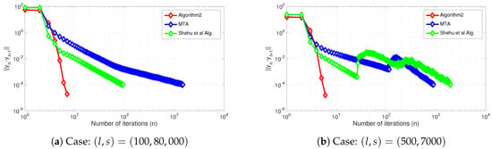
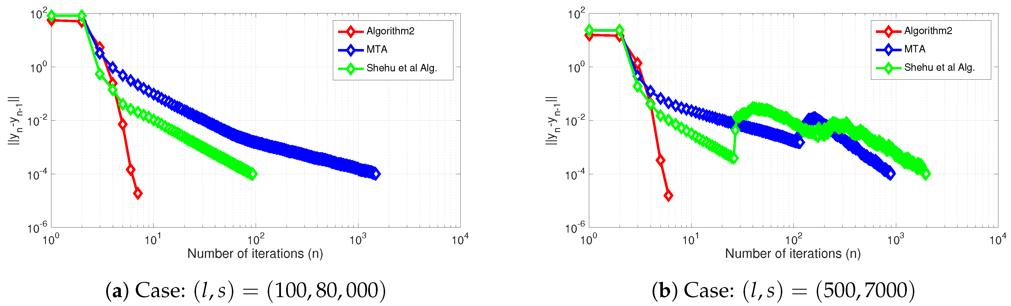
Figure 1 shows the behavior of $\parallel y_k-y_{k-1}\parallel$ for Algorithm 2, MTA, and Shehu et al.’s algorithm in Equation (3) in two different choices of $(l,s)$. We can observe that by using our algorithm the behavior of the red line, and Algorithm 2 has the best performance.

Figure 1. Illustration the behavior of $\parallel y_n-y_{n-1}\parallel$ for Algorithm 2, MTA, and Shehu et al.’s algorithm in Equation (3).

5.2. Image Restoration Problems

In this subsection, we apply the proposed algorithm, image restoration problems, which involves deblurring and denoising images. We consider the degradation model that represents an actual image restoration problems or through the least useful mathematical abstractions thereof.

$$y=Hx+w,$$

(23)

where $y,H,x$ and w represent the degraded image, degradation operator, or blurring operator; original image; and noise operator, respectively.

The reconstructed image is obtained by solving the following regularized least-squares problem

$$\underset{x}{min}\left\{\frac{1}{2}{\parallel Hx-y\parallel }_2^2+\mu \varphi \left(x\right)\right\},$$

(24)

where $\mu >0$ is the regularization parameter and $\varphi (·)$ is the regularization functional. A well-known regularization function used to remove noise in the restoration problem is the $l_1$ norm, which is called Tikhonov regularization [36]. The problem in Equation (24) can be written in the form of the following problem as:

$$\mathrm{find}x\in \underset{x\in {\mathbb{R}}^k}{argmin}\left\{\frac{1}{2}{\parallel Hx-y\parallel }_2^2+\mu {\parallel x\parallel }_1\right\},$$

(25)

where y is the degraded image and H is a bounded linear operator. Note that problem in Equation (25) is a spacial case of the problem in Equation (4) by setting $A=\partial f(·)$, $B=0$, and $C=\nabla L(·)$ where $f\left(x\right)={\parallel x\parallel }_1$ and $L\left(x\right)=\frac{1}{2}{\parallel Hx-y\parallel }_2^2$. This setting we have that $C\left(x\right)=\nabla L\left(x\right)=H^{*}(Hx-y)$, where $H^{*}$ is a transpose of H. We begin the problem by choosing images and degrade them by random noise and different types of blurring. The random noise in this study is provided by Gaussian white noise of zero mean and $0.001$ variance. We solve the problem in Equation (25) by using our algorithm in Corollary 2. We set ${\alpha }_n=1-\frac{1}{{(n+1)}^2},{\delta }_n=1-\frac{1}{100n+1},\mu =0.001,{\epsilon }_n=0$ and ${\theta }_n$ is defined as Equation (22).

We compare our proposed algorithm with the inertial Mann-type algorithm that was introduced by Kitkuan et al. [30]. In Kitkuan et al.’s algorithm (Algorithm in Theorem 3.1 in [30]), we choose ${\varsigma }_n={\theta }_n,{\alpha }_n=\frac{1}{n+1},{\lambda }_n=0.001$, and $h\left(x\right)=\frac{1}{12}{\parallel x\parallel }_2^2$. We assess the quality of the reconstructed image by using the signal to noise ratio (SNR) for monochrome images, which is defined by

$$\mathbf{SNR}\left(n\right)=20{log}_{10}\frac{{\parallel x\parallel }_2^2}{\parallel x-x_n{\parallel }_2^2},$$

where x and $x_n$ denote the original and the restored image at iteration n, respectively.

For color images, we estimate the quality of the reconstructed image by using the normalized color difference (NCD) [37] which is defined by

$$\mathbf{NCD}\left(n\right)=\frac{{\sum }_{i=1}^N{\sum }_{j=1}^M\sqrt{{(L_{i,j}^o-L_{i,j}\left(n\right))}^2+{(u_{i,j}^o-u_{i,j}\left(n\right))}^2+{(v_{i,j}^o-v_{i,j}\left(n\right))}^2}}{{\sum }_{i=1}^N{\sum }_{j=1}^M\sqrt{{\left(L_{i,j}^o\right)}^2+{\left(u_{i,j}^o\right)}^2+{\left(v_{i,j}^o\right)}^2}},$$

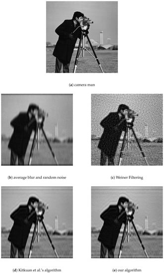
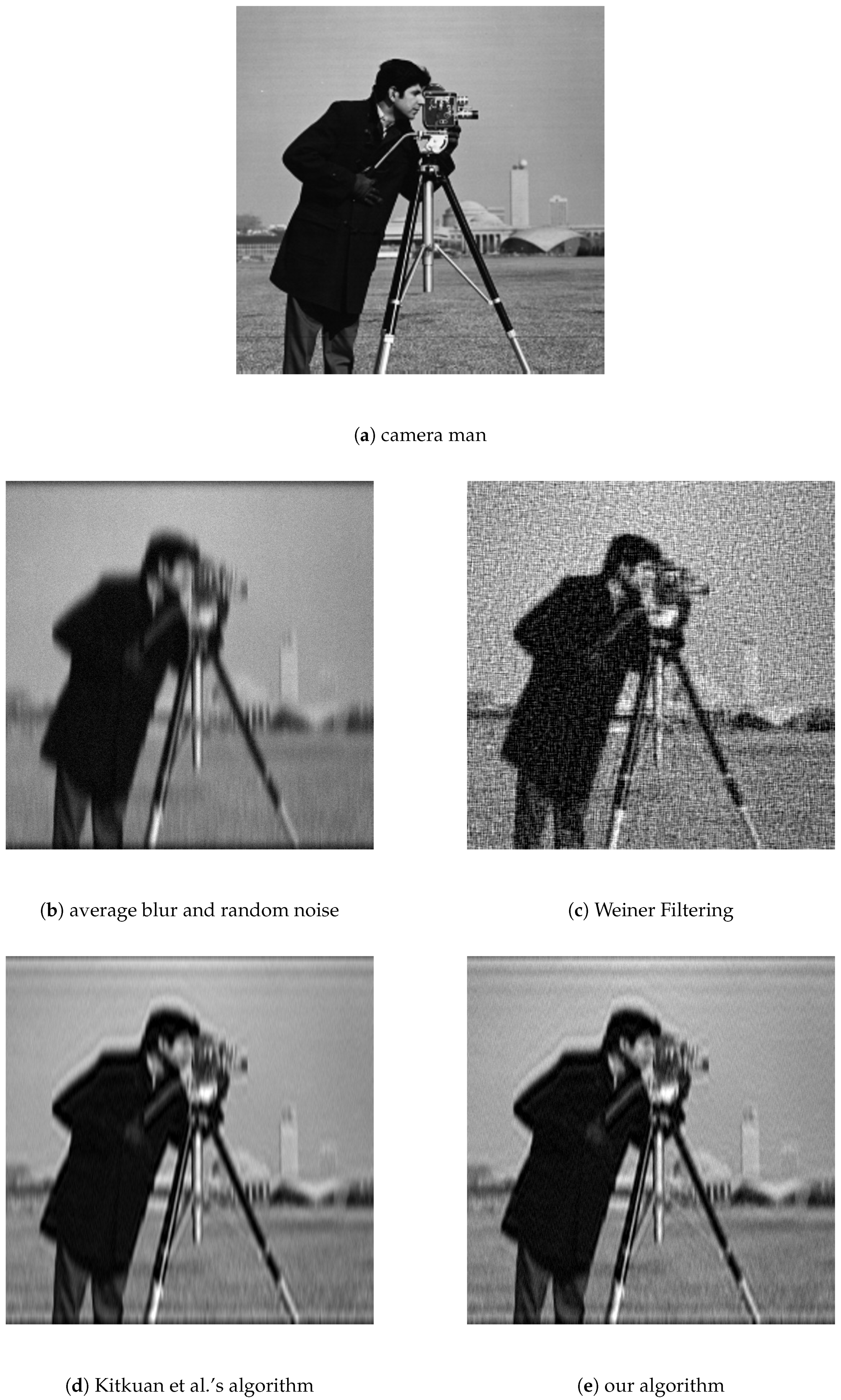
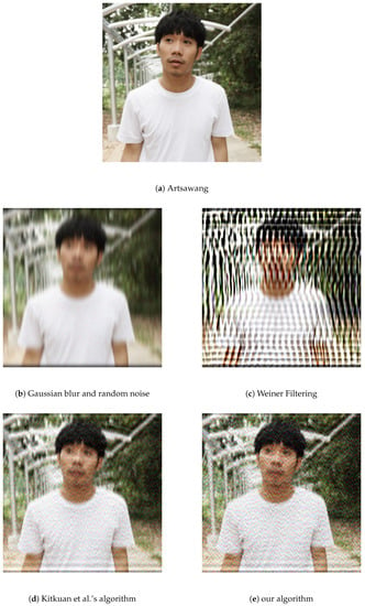
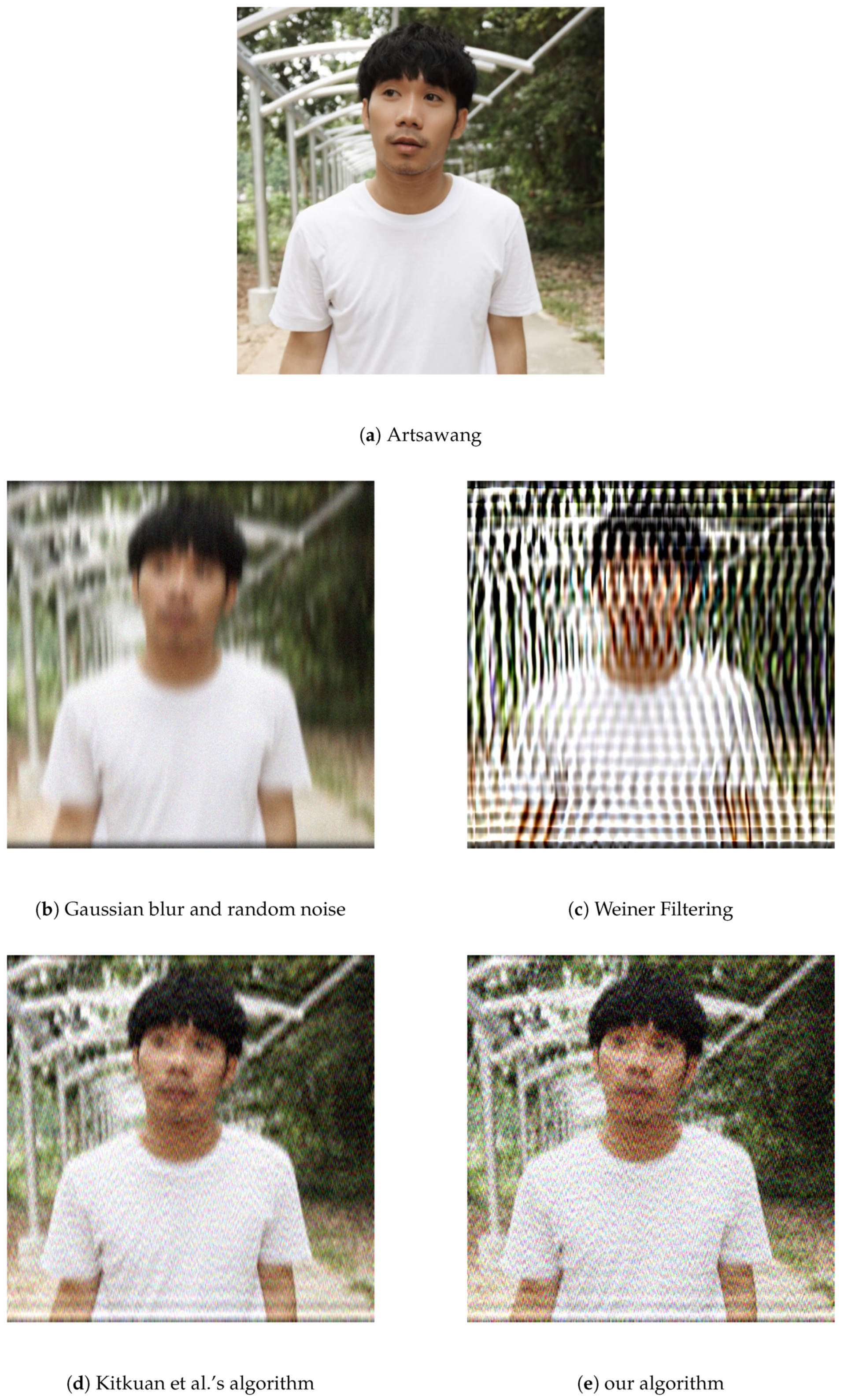
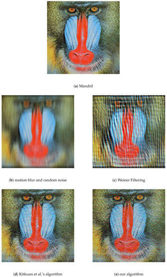
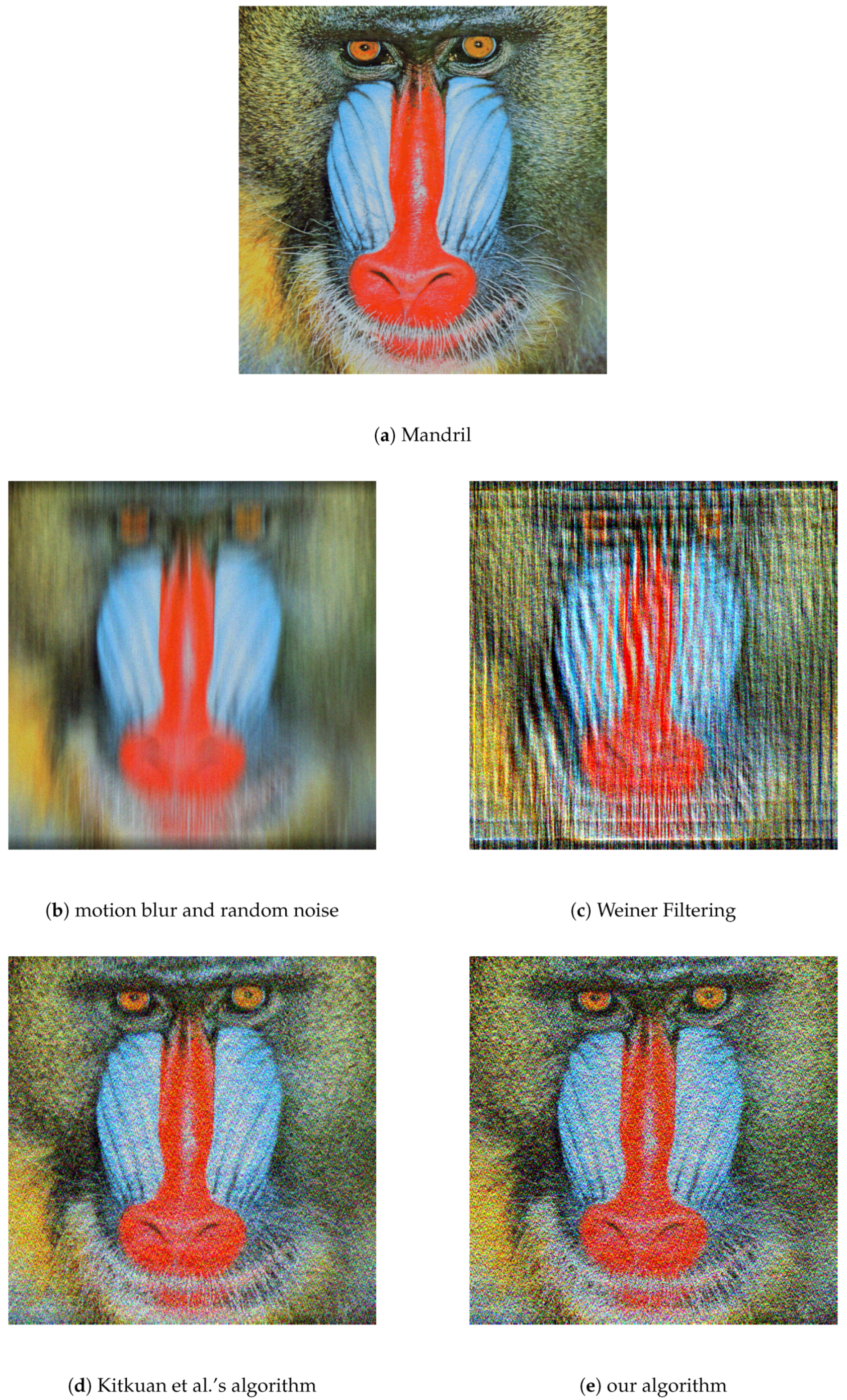
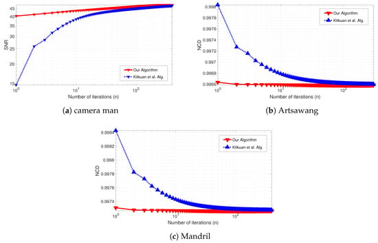
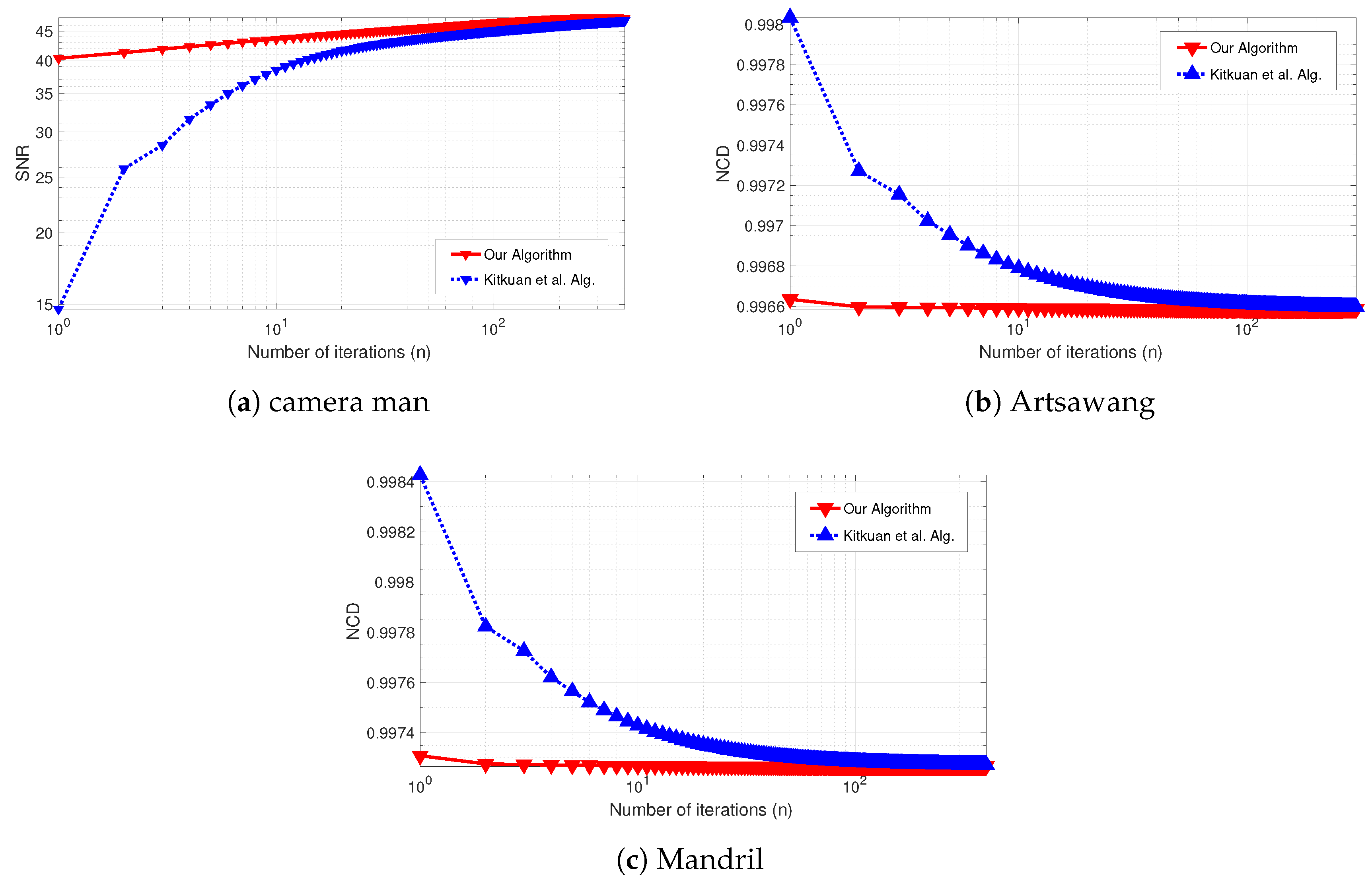
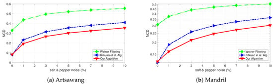
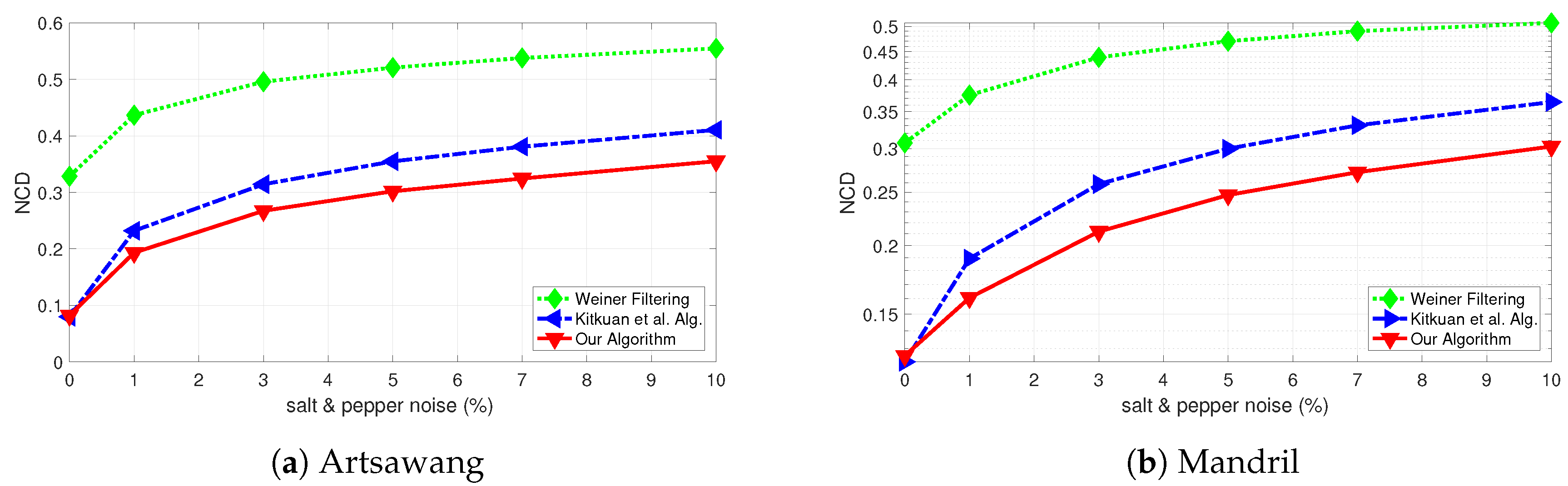
where $i,j$ are indices of the sample position, $N,M$ characterize an image size and $L_{i,j}^o,u_{i,j}^o,v_{i,j}^o$ and $L_{i,j}\left(n\right),u_{i,j}\left(n\right),v_{i,j}\left(n\right)$ are values of the perceived lightness and two representatives of chrominance related to the original and the restored image at iteration n, respectively. We generated the noised model in order to obviously see the differences between degraded and original figure as follows. Figure 2 firstly shows the original image. Secondly, the degraded image was corrupted by average blur (size 20 by 20) and Gaussian noise (zero mean and 0.001 variance). We randomly selected parameters which visibly showed the differences sharpness level and. Lastly, reconstructed images are shown. Figure 3 firstly shows the original image. Secondly, the degraded image was corrupted by Gaussian blur (size 20 by 20 with the standard deviation 20) and Gaussian noise (zero mean and 0.001 variance). With this point, we found that any adjustment of the standard deviation as much as small might not shown the difference between degraded and original figure. Lastly, reconstructed images are shown. Figure 4 firstly shows the original image. Secondly, the degraded image was corrupted by motion blur (the linear motion of a camera by 30 pixels with an angle of 60 degrees) and Gaussian noise (zero mean and 0.001 variance). We randomly selected parameters which visibly showed the differences sharpness level. Lastly, reconstructed images are shown. The comparisons between our proposed algorithm in Equation (19) and Kitkuan et al.’s algorithm (Algorithm in Theorem 3.1 in [30]) in image restoration problems are presented in Figure 5 and Table 2. Furthermore, we also present the comparison of Kitkuan et al.’s algorithm (Algorithm in Theorem 3.1 in [30]), our algorithm, and the well-known technique for image restoration which is Weiner filtering (WF) [38,39]. Figure 6 presents the comparative results of two degradation images ’Artsawang’ and ’Mandril’ corrupted by motion blur and different salt and pepper noise from $0\%$ to $10\%$.

Figure 2. (a) The original image ‘camera man’; (b) the images degraded by average blur and random noise (Gaussian noise); and (c–e) the reconstructed image by using Weiner filter, Kitkuan et al.’s algorithm, and our algorithm in Equation (19), respectively.

Figure 3. (a) The original image ‘Artsawang’; (b) the images degraded by Gaussian blur and random noise (Gaussian noise); and (c–e) the reconstructed image by using Weiner filter, Kitkuan et al.’s algorithm, and our algorithm in Equation (19), respectively.

Figure 4. (a) The original image ‘Mandril’; (b) the images degraded by motion blur and random noise (Gaussian noise); and (c–e) the reconstructed image by usingWeiner filter, Kitkuan et al.’s algorithm, and our algorithm in Equation (19), respectively.

Figure 5. (a) The behavior of SNR for two algorithms in Figure 2d,e; (b) the behavior of NCD for two algorithms in Figure 3d,e; and (c) the behavior of NCD for two algorithms in Figure 4d,e.

Table 2. The performance of the normalized color difference (NCD) in two images.

The Normalized Color Difference (NCD).
	Kitkuan et al.’s Algorithm		Our Algorithm in Equation (19)
$\mathit{n}$	Artsawang Image	Mandril Image	Artsawang Image	Mandril Image
1	0.99803	0.99842	0.99663	0.99731
50	0.99660	0.99730	0.99659	0.99727
100	0.99661	0.99729	0.99658	0.99726
200	0.99660	0.99728	0.99658	0.99726
300	0.99659	0.99727	0.99658	0.99726
400	0.99659	0.99727	0.99658	0.99726

Figure 6. (a,b) The behavior of NCD in motion blur and different different salt and pepper noise from 0% to 10%.

6. Conclusions

In this paper, we propose a new Mann-type method combining both inertial terms and errors to solve the fixed point problem for a nonexpansive mapping. We also prove the strong convergence of the proposed algorithm under some sufficient conditions of involved parameters. We also apply results to approximate the solutions of the monotone inclusion problems. Furthermore, we also provide a numerical example to compare the proposed algorithm with other algorithms in the convex minimization problem. Finally, we use our method to solve image restoration problems.

References

- Bauschke, H.H.; Combettes, P.L. Convex Analysis and Monotone Operator Theory in Hilbert Spaces; CMS Books in Mathematics; Springer: New York, NY, USA, 2011. [Google Scholar]
- Bagiror, A.; Karmitsa, N.; Mäkelä, M.M. Introduction to Nonsmooth Optimization: Theory, Practice and Software; Springer: New York, NY, USA, 2014. [Google Scholar]
- Mann, W.R. Mean value methods in iteration. Proc. Am. Math. Soc. 1953, 4, 506–510. [Google Scholar] [CrossRef]
- Bauschke, H.H.; Combettes, P.L. A weak-to-strong convergence principle for fejer-monotone methods in Hilbert spaces. Math. Oper. Res. 2001, 26, 248–264. [Google Scholar] [CrossRef] [Scilit]
- Reich, S. Weak convergence theorems for nonexpansive mappings in Banach spaces. J. Math. Anal. Appl. 1979, 67, 274–276. [Google Scholar] [CrossRef] [Scilit]
- Halpern, B. Fixed points of nonexpansive maps. Bull. Am. Math. Soc. 1967, 73, 957–961. [Google Scholar] [CrossRef] [Scilit]
- Shioji, N.; Takahashi, W. Strong convergence of approximated sequences for nonexpansive mapping in Banach spaces. Proc. Am. Math. Soc. 1997, 125, 3641–3645. [Google Scholar] [CrossRef] [Scilit]
- Chidume, C.E.; Chidume, C.O. Iterative approximation of fixed points of nonexpansive mappings. J. Math. Anal. Appl. 2006, 318, 288–295. [Google Scholar] [CrossRef] [Scilit]
- Cholamjiak, P. A generalized forward-backward splitting method for solving quasi inclusion problems in Banach spaces. Numer. Algorithms 2016, 71, 915–932. [Google Scholar] [CrossRef] [Scilit]
- Lions, P.-L. Approximation de points fixes de contractions. CR Acad. Sci. Paris Sér. 1977, 284, A1357–A1359. [Google Scholar]
- Reich, S. Strong convergence theorems for resolvents of accretive operators in Banach spaces. J. Math. Anal. Appl. 1980, 75, 287–292. [Google Scholar] [CrossRef] [Scilit]
- Reich, S. Some problems and results in fixed point theory. Contemp. Math. 1983, 21, 179–187. [Google Scholar]
- Wittmann, R. Approximation of fixed points of nonexpansive mappings. Arch. Math. 1992, 58, 486–491. [Google Scholar] [CrossRef] [Scilit]
- Xu, H.-K. Iterative algorithms for nonlinear operators. J. Lond. Math. Soc. 2002, 66, 240–256. [Google Scholar] [CrossRef] [Scilit]
- Moudafi, A. Viscosity approximation methods for fixed points problems. J. Math. Anal. Appl. 2000, 241, 46–55. [Google Scholar] [CrossRef] [Scilit]
- Dong, Q.L.; Lu, Y.Y. A new hybrid algorithm for a nonexpansive mapping. Fixed Point Theroy Appl. 2015, 2015, 37. [Google Scholar] [CrossRef] [Scilit]
- Dong, Q.L.; Yuan, H.B. Accelerated Mann and CQ algorithms for finding a fixed point of a nonexpansive mapping. Fixed Point Theroy Appl. 2015, 2015, 125. [Google Scholar] [CrossRef] [Scilit]
- Kanzow, C.; Shehu, Y. Generalized Krasnoselskii-Mann-type iterations for nonexpansive mappings in Hilbert spaces. Comput. Optim. Appl. 2017, 67, 595–620. [Google Scholar] [CrossRef] [Scilit]
- Kim, T.H.; Xu, H.K. Strong convergence of modified Mann iterations. Non-Linear Anal. 2005, 61, 51–60. [Google Scholar] [CrossRef] [Scilit]
- Takahashi, W. Nonlinear Functional Analysis; Yokohama Publishers: Yokohama, Japan, 2000. [Google Scholar]
- Boţ, R.I.; Csetnek, E.R.; Meier, D. Inducing strong convergence into the asymptotic behaviour of proximal splitting algorithms in Hilbert spaces. Optim. Methods Softw. 2019. [Google Scholar] [CrossRef] [Scilit]
- Polyak, B.T. Some methods of speeding up the convergence of iterative methods. Zh. Vychisl. Mat. Mat. Fiz. 1964, 4, 1–17. [Google Scholar]
- Boţ, R.I.; Csetnek, E.R.; Hendrich, C. Inertial Douglas-Rachford splitting for monotone inclusion problems. Appl. Math. Comput. 2015, 256, 472–487. [Google Scholar] [CrossRef] [Scilit]
- Boţ, R.I.; Csetnek, E.R.; László, S. An inertial forward-backward algorithm for the minimization of the sum of two nonconvex functions. EURO J. Comput. Optim. 2016, 4, 3–25. [Google Scholar] [CrossRef] [Scilit]
- Boţ, R.I.; Csetnek, E.R.; Nimana, N. Gradient-type penalty method with inertial effects for solving constrained convex optimization problems with smooth data. Optim. Lett. 2017. [Google Scholar] [CrossRef] [Scilit] [PubMed]
- Boţ, R.I.; Csetnek, E.R.; Nimana, N. An Inertial Proximal-Gradient Penalization Scheme for Constrained Convex Optimization Problems. Vietnam J. Math. 2017, 46, 53–71. [Google Scholar] [CrossRef] [Scilit]
- Cholamjiak, W.; Cholamjiak, P.; Suantai, S. An inertial forward-backward splitting method for solving inclusion problems in Hilbert spaces. J. Fixed Point Theory Appl. 2018, 2018. [Google Scholar] [CrossRef] [Scilit]
- Cholamjiak, P.; Shehu, Y. Inertial forward-backward splitting method in Banach spaces with application to compressed sensing. Appl. Math. 2019, 64, 409–435. [Google Scholar] [CrossRef] [Scilit]
- Kitkuan, D.; Kumam, P.; Martínez-Moreno, J. Generalized Halpern-type forward-backward splitting methods for convex minimization problems with application to image restoration problems. Optimization 2019. [Google Scholar] [CrossRef] [Scilit]
- Kitkuan, D.; Kumam, P.; Martínez-Moreno, J.; Sitthithakerngkiet, K. Inertial viscosity forward–backward splitting algorithm for monotone inclusions and its application to image restoration problems. Int. J. Comput. Math. 2020, 97, 1–19. [Google Scholar] [CrossRef] [Scilit]
- Mainge, P.E. Convergence theorems for inertial KM-type algorithms. J. Comput. Appl. Math. 2008, 219, 223–236. [Google Scholar] [CrossRef] [Scilit]
- Combettes, P.L.; Yamada, I. Compositions and convex combinations of averaged nonexpansive operators. J. Math. Anal. Appl. 2015, 425, 55–70. [Google Scholar] [CrossRef] [Scilit]
- Shehu, Y.; Iyiola, O.S.; Ogbuisi, F.U. Iterative method with inertial terms for nonexpansive mappings: Applications to compressed sensing. Numer. Algorithms 2019. [Google Scholar] [CrossRef] [Scilit]
- Davis, D.; Yin, W. A Three-Operator Splitting Scheme and its Optimization Applications. Set-Valued Var. Anal. 2017, 25, 829–858. [Google Scholar] [CrossRef] [Scilit]
- Mainge, P.E. Approximation methods for common fixed points of nonexpansive mappings in Hilbert spaces. J. Math. Anal. Appl. 2007, 325, 469–479. [Google Scholar] [CrossRef] [Scilit]
- Tikhonov, A.N.; Arsenin, V.Y. Solutions of Ill—Posed Problems. SIAM Rev. 1979, 21, 266–267. [Google Scholar]
- Ma, Z.; Wu, H.R. Partition based vector filtering technique for color suppression of noise in digital color images. IEEE Trans. Image Process. 2006, 15, 2324–2342. [Google Scholar]
- Lim, J.S. Two-Dimensional Signal Processing; Prentice-Hall: Englewood Cliffs, NJ, USA, 1990. [Google Scholar]
- Gonzalez, R.C.; Woods, R.E. Digital Image Processing, 4th ed.; Prentice-Hall: Englewood Cliffs, NJ, USA, 2017. [Google Scholar]
© 2020 by the authors. Licensee MDPI, Basel, Switzerland. This article is an open access article distributed under the terms and conditions of the Creative Commons Attribution (CC BY) license (http://creativecommons.org/licenses/by/4.0/).