Dynamical Behavior of a Stochastic SIRC Model for Influenza A

Abstract

In this paper, a stochastic SIRC epidemic model for Influenza A is proposed and investigated. First, we prove that the system exists a unique global positive solution. Second, the extinction of the disease is explored and the sufficient conditions for extinction of the disease are derived. And then the existence of a unique ergodic stationary distribution of the positive solutions for the system is discussed by constructing stochastic Lyapunov function. Furthermore, numerical simulations are employed to illustrate the theoretical results. Finally, we give some further discussions about the system.

1. Introduction

Influenza is an infectious disease characterized by acute respiratory infection caused by the RNA influenza virus of the mucinous virus family [1,2]. The clinical features of influenza are fever, headache, myalgia, fatigue, nasal congestion, sore throat and cough, and the severity of the disease varies [3]. The complications and deaths caused by the flu are very serious. The flu can aggravate the underlying diseases such as cardiopulmonary diseases, and can also cause primary influenza virus pneumonia or secondary bacterial pneumonia. According to estimates by the World Health Organization, about 20% of children and 5% of adults worldwide are infected with the flu each year, and the global pandemic causes approximately 3 million to 5 million serious cases each year and approximately 290,000 to 650,000 deaths related to respiratory diseases [4]. Prevention of influenza is an important global public health issue. The use of vaccines provides an effective guarantee for the prevention and control of influenza, and has achieved remarkable results.

According to the antigenicity of nuclear proteins and matrix proteins, influenza viruses can be generally divided into three types: A, B, and C [5]. In 2011, virologists first isolated influenza D virus from pigs in Oklahoma, USA [6]. The influenza virus is also isolated in sheep and goats [7,8,9,10]. Every type contains a wide variety of subtypes according to hemagglutinin (HA) and neuraminidase (NA) differences [11]. Influenza A virus can be divided into 18 different HA subtypes (H1-H18) and 9 different NA subtypes (N1-N9) [12]. Among them, only H1N1, H2N2, and H3N2 mainly infect humans, and many other subtypes of natural hosts are a variety of birds and animals. Among them, H5, H7 and H9 subtype strains are the most harmful to birds. Under normal circumstances, the avian flu virus does not infect animals other than birds and pigs. However, in 1997, Hong Kong reported for the first time 18 cases of H5N1 human avian influenza infection, of which 6 cases died, causing widespread concern worldwide. Since 1997, there have been several incidents of avian influenza virus infection in the world. Avian influenza viruses such as H5N1, H7N7, H7N9, and H9N2 with high pathogenicity, once mutated and having human-to-human transmission ability, will lead to human bird flu epidemic, indicating that bird flu virus has a great potential threat to humans. Influenza A is highly pathogenic to humans and has caused worldwide pandemics. Among the influenza A viruses, the avian influenza virus subtypes that have been found to directly infect humans are: H1N1, H5N1, H7N1, H7N2, H7N3, H7N7, H7N9, H9N2 and H10N8. Among them, H1, H5 and H7 subtypes are highly pathogenic, and H1N1, H5N1 and H7N9 are particularly worthy of attention [13].

Mathematical modeling plays an part role in the study of the spread of epidemic diseases. Mathematical models can provide a more typical, more refined, and more quantitative description of complex epidemics. Mathematical models find the various theoretical indicators of disease transmission by studying the rate of change of disease state variables, and use these indicators to analyze the characteristics and patterns of different disease epidemics, simulate the process of disease epidemics under various conditions, predict the possible epidemic trends, and simulate and evaluate the effects of different prevention strategies and measures. Then based on the classical SIR modes, a large number of mathematical models were established to model the evolution of epidemic diseases, such as influenza A, tuberculosis, measles, hand-foot-mouth disease, etc [14,15,16,17,18]. However, the antigenic variation of influenza viruses is very frequent, by constantly changing the antigenicity, the flu virus can escape the attack of the host immune system. Mutations in the two important glycoproteins on the surface of influenza viruses, hemagglutinin (HA) and neuraminidase (NA) are the main causes of variability in influenza viruses. According to the degree of antigenic variation, it can be divided into antigenic drift and antigenic shift. The former is caused by point mutation and can cause seasonal influenza epidemic. The latter is caused by genetic recombination, which may produce a new influenza pandemic [5,19,20].

Recently, considering the cross-immunity phenomenon during the spread of influenza A [21,22,23], Casagrandi et al. [24] proposed an SIRC model as follows,

$$\left\{\begin{array}{c}{\displaystyle \dot{S}\left(t\right)=\mu (1-S\left(t\right))-\beta S\left(t\right)I\left(t\right)+\gamma C\left(t\right),}\hfill \\ {\displaystyle \dot{I}\left(t\right)=\beta S\left(t\right)I\left(t\right)+p\beta C\left(t\right)I\left(t\right)-(\mu +\alpha )I\left(t\right),}\hfill \\ {\displaystyle \dot{R}\left(t\right)=(1-p)\beta C\left(t\right)I\left(t\right)+\alpha I\left(t\right)-(\mu +\delta )R\left(t\right),}\hfill \\ {\displaystyle \dot{C}\left(t\right)=\delta R\left(t\right)-\beta C\left(t\right)I\left(t\right)-(\mu +\gamma )C\left(t\right),}\hfill \end{array}\right.$$

(1)

where $S\left(t\right)$, $I\left(t\right)$, $R\left(t\right)$ and $C\left(t\right)$ are the sizes of susceptible, infected, recovered and cross-immune individuals, respectively. $\mu$ is the death rate in every compartment. $\beta$ is the contact rate. $\gamma$ is the rate at which cross-immune populations lose immunity and become susceptible. p is the rate at which cross-immune populations become infected by reinfection. $\alpha$ is the recovery rate. $\delta$ is the cross-immunity acquisition rate. All parameter values are nonnegative.

Li and Guo [25] have given a completed stability analysis of the equilibria of model (1) based on the basic reproduction number $R_0=\frac{\beta }{\mu +\alpha },$ and if $R_0<1,$ system (1) has a unique globally asymptotically stable disease-free equilibrium $E_0=(1,0,0,0),$ and on the other hand, if $R_0>1,$ $E_0$ lost its stability and system (1) has a unique globally asymptotically stable endemic equilibrium $E^{\ast }=(S^{\ast },I^{\ast },R^{\ast },C^{\ast }).$

However, there are stochastic factors everywhere in nature, so it makes sense to study biological models with stochastic factors because random factors provide one more dimension, for example, Zhu et al. [26], Zhang and Zhang [27], Liu et al. [28] and Chi and Zhao [29] have considered stochastic effect on population. In particular, infectious diseases are inevitably affected by stochastic factors during the process of transmission. Compared with deterministic epidemic models, stochastic epidemic models can better reflect the evolution of infectious diseases in nature. According to the way of considering different stochastic disturbances, many scholars have established a variety of stochastic infectious disease models, and investigated the asymptotic behavior of the system. For example, the impact of environmental disturbances on the rate of transmission have been considered based on SIR (Susceptible-Infected-Recovered) [30,31,32,33,34,35,36], SIS (Susceptible-Infected-Susceptible) [37,38,39,40,41,42] and SIRS (Susceptible-Infected-Recovered-Susceptible) model [43,44,45,46]. However, the above literatures on infectious diseases have evolved mainly among the three compartments (S, I and R). According to the study in [24], cross-immunity causes complex transmission of infectious diseases. Then based on model (1), we consider the impact of environmental disturbances on SIRC model and get a stochastic SIRC model as follows:

$$\left\{\begin{array}{c}{\displaystyle \mathrm{d}S\left(t\right)=\left[\mu (1-S(t\left)\right)-\beta S\left(t\right)I\left(t\right)+\gamma C\left(t\right)\right]\mathrm{d}t+{\sigma }_{1}S\left(t\right)\mathrm{d}{B}_1\left(t\right),}\hfill \\ {\displaystyle \mathrm{d}I\left(t\right)=\left[\beta S\left(t\right)I\left(t\right)+p\beta C\left(t\right)I\left(t\right)-(\mu +\alpha )I\left(t\right)\right]\mathrm{d}t+{\sigma }_{2}I\left(t\right)\mathrm{d}{B}_2\left(t\right),}\hfill \\ {\displaystyle \mathrm{d}R\left(t\right)=\left[(1-p)\beta C\left(t\right)I\left(t\right)+\alpha I\left(t\right)-(\mu +\delta )R\left(t\right)\right]\mathrm{d}t+{\sigma }_{3}R\left(t\right)\mathrm{d}{B}_3\left(t\right),}\hfill \\ {\displaystyle \mathrm{d}C\left(t\right)=\left[\delta R\left(t\right)-\beta C\left(t\right)I\left(t\right)-(\mu +\gamma )C\left(t\right)\right]\mathrm{d}t+{\sigma }_{4}C\left(t\right)\mathrm{d}{B}_4\left(t\right),}\hfill \end{array}\right.$$

(2)

where $B_i\left(t\right)$ are independent standard Brownian motions and $B_i\left(0\right)=0(i=1,2,3,4),$ the corresponding stochastic integrals w.r.t. the Brownian motions under consideration are all of the Itô typ, and ${\sigma }_i>0(i=1,2,3,4)$ represent the intensities of the noise to the susceptible, infected, recovered and cross-immune, respectively.

The main text is organised as follows. The extinction conditions of the disease are explored In Section 4. The existence of stationary distribution as well as the ergodic property is discussed under certain sufficient conditions in Section 5. We present some numerical examples to illustrate the theoretical results in Section 6, and some further discussion of the model is given in Section 7.

2. Preliminaries

In this section, we introduce some essential theory with respect to stochastic differential equations (SDEs) which can be found in [47,48]. Let $\Omega$ is a nonempty set, also known as sample space, then $(\Omega ,\mathcal{F},\mathbb{P})$ is called a complete probability space with a filtration ${\left\{{\mathcal{F}}_t\right\}}_{t\ge 0}$ satisfying the usual conditions. The functions $B_i\left(t\right)(i=1,2,3,4)$ are defined on $(\Omega ,\mathcal{F},\mathbb{P})$ and we also let ${\mathbb{R}}_{+}^l=\{y\in {\mathbb{R}}^l:y_i>0,1\le i\le l\},$$E_l$ denote l-dimensional Euclidean space and $\langle g\left(t\right)\rangle =\frac{1}{t}{\int }_0^{t}g\left(s\right)ds.$

Next, let us consider the l-dimensional SDE

$$\mathrm{d}Y\left(t\right)=g(Y\left(t\right),t)\mathrm{d}t+h(Y\left(t\right),t)\mathrm{d}B\left(t\right),t\ge t_0,$$

(3)

with initial value $y\left(t_0\right)=y_0\in {\mathbb{R}}^l.$

Define a differential operator $\mathcal{L}$ [47] of (3) as

$$\mathcal{L}=\frac{\partial }{\partial t}+\sum g_i(Y,t)\frac{\partial }{\partial Y_i}+\frac{1}{2}\sum _{i,j=1}^l{\left[h^T(Y,t)h(Y,t)\right]}_{ij}\frac{{\partial }^2}{\partial Y_i\partial Y_j}.$$

(4)

If $\mathcal{L}$ acts on a function $V\in C^{2,1}({\mathbb{R}}^l\times [t_0,\infty ];{\mathbb{R}}_{+}),$ then

$$\mathcal{L}V(Y,t)=V_t(Y,t)+V_Y(Y,t)g(Y,t)+\frac{1}{2}\mathrm{trace}\left[h^T(Y,t)V_{YY}(Y,t)h(Y,t)\right],$$

(5)

where $V_t=\frac{\partial V}{\partial t},V_Y=(\frac{\partial V}{\partial y_1},\cdots ,\frac{\partial V}{\partial y_l}),V_{YY}={\left(\frac{{\partial }^{2}V}{\partial Y_i\partial Y_j}\right)}_{l\times l}.$ Appling Itô’s formula, one gets

$$\mathrm{d}V(Y\left(t\right),t)=\mathcal{L}V(y\left(t\right),t)\mathrm{d}t+V_Y(Y\left(t\right),t)h(Y\left(t\right),t)\mathrm{d}B\left(t\right),$$

(6)

where $Y\left(t\right)\in {\mathbb{R}}^l.$

Let $Y\left(t\right)$ be a homogenous Markov process in $E_l,$ and be expressed by

$$\mathrm{d}Y\left(t\right)=b\left(Y\right)dt+\sum _{r=1}^k{h}_r\left(Y\right)\mathrm{d}{B}_r\left(t\right),$$

(7)

then

$$A\left(y\right)=\left(a_{ij}\left(y\right)\right),a_{ij}\left(y\right)=\sum _{r=1}^k{h}_r^i\left(y\right)h_r^j\left(y\right)$$

(8)

is defined as the diffusion matrix.

Lemma 1.

([49]) For any solution $\left(S\right(t),I(t),R(t),$ $C\left(t\right))\in {\mathbb{R}}_{+}^4$ of model (2) with initial value $(S\left(0\right),I\left(0\right),R\left(0\right),C\left(0\right))\in {\mathbb{R}}_{+}^4,$ we have the following results:

$$\underset{t\to \infty }{lim}\frac{S\left(t\right)}{t}=0,\underset{t\to \infty }{lim}\frac{I\left(t\right)}{t}=0,\underset{t\to \infty }{lim}\frac{R\left(t\right)}{t}=0,\underset{t\to \infty }{lim}\frac{C\left(t\right)}{t}=0a.s.$$

3. Global Existence and Uniqueness of the Positive Solution

Theorem 1.

For any given initial value $(S\left(0\right),I\left(0\right),R\left(0\right),C\left(0\right))\in {\mathbb{R}}_{+}^4,$ there exists a unique global positive solution $\left(S\right(t),I(t),R(t),C(t\left)\right)$ of system (2) on $t\ge 0.$

Proof. 

First, we show the solution exists locally. In fact, the solution exists locally on $t\in [0,{\tau }_{exp}),$ here ${\tau }_{exp}$ is the explosion time, since the coefficients satisfy the local Lipschitz conditions.

Next, we show the solution exists globally. Let $k_0>0$ large enough for any initial value $S\left(0\right),I\left(0\right),R\left(0\right)$ and $C\left(0\right)$ in $[\frac{1}{k_0},k].$ To each integer $k\ge k_0,$ let us consider the following stopping time

$$\begin{array}{c}\hfill {\tau }_k=inf\left\{t\in [0,{\tau }_e):min\{S\left(t\right),I\left(t\right),R\left(t\right),C\left(t\right)\}\le \frac{1}{k}\mathrm{or}max\{S\left(t\right),I\left(t\right),R\left(t\right),C\left(t\right)\}\ge k\right\},\end{array}$$

Let $infØ=\infty ,$ where Ø is the empty set. Obsviously, ${\tau }_k$ is increasing as $k\to \infty .$ Denote ${lim}_{k\to \infty }{\tau }_k={\tau }_{\infty },$ then ${\tau }_{\infty }\ge {\tau }_k$ a.s. Next, let us verify ${\tau }_{\infty }=\infty$ a.s., if not, there must exist two constants $T>0$ and $ϵ\in (0,1)$ such that $\mathbb{P}\{{\tau }_{\infty }\le T\}>ϵ.$ Thus there exists an integer $k_1\ge k_0$ such that $\mathbb{P}\{{\tau }_k\le T\}\ge ϵ,k\ge k_1.$ Let us define a $C^2$-function V: ${\mathbb{R}}_{+}^4\to {\mathbb{R}}_{+}$ as follows:

$$V=S-a-aln\frac{S}{a}+I-1-lnI+R-1-lnR+C-a-aln\frac{C}{a},$$

(9)

applying Itô’s formula, one gets

$$\begin{array}{cc}\hfill \mathrm{d}V=& \mathcal{L}V\mathrm{d}t+{\sigma }_1(S-a)\mathrm{d}{B}_1\left(t\right)+{\sigma }_2(I-1)\mathrm{d}{B}_2\left(t\right)+{\sigma }_3(R-1)\mathrm{d}{B}_3\left(t\right)+{\sigma }_4(C-a)\mathrm{d}{B}_4\left(t\right),\hfill \end{array}$$

(10)

where

$$\begin{array}{cc}\hfill \mathcal{L}V=& \left(1-\frac{a}{S}\right)\left[\mu (1-S)-\beta SI+\gamma C\right]+\frac{1}{2}{a}_1{\sigma }_1^2\hfill \\ \hfill & +\left(1-\frac{1}{I}\right)\left[\beta SI+p\beta CI-(\mu +\alpha )I\right]+\frac{{\sigma }_2^2}{2}\hfill \\ \hfill & +\left(1-\frac{1}{R}\right)\left[(1-p)\beta CI+\alpha I-(\mu +\delta )R\right]+\frac{{\sigma }_3^2}{2}\hfill \\ \hfill & +\left(1-\frac{a}{C}\right)\left[\delta R-\beta CI-(\mu +\gamma )C\right]+\frac{{\sigma }_4^2}{2}\hfill \\ \hfill =& \mu -\mu (S+I+R+C)-\frac{a\mu }{S}+a\mu +a\beta I-\frac{a\gamma C}{S}-\beta S-p\beta C+\mu +\alpha \hfill \\ \hfill & -(1-p)\beta \frac{CI}{R}-\frac{\alpha I}{R}+\mu +\delta -\frac{a\delta R}{C}+a\beta I+a\mu +a\gamma \hfill \\ \hfill \le & (2a\beta -\mu )I+(3+2a)\mu +\alpha +\delta +a\gamma .\hfill \end{array}$$

(11)

Choose $a=\frac{\mu }{2\beta }$ such that $2a\beta -\mu =0$, then

$$\mathcal{L}V\le (3+\frac{\mu }{\beta })\mu +\alpha +\delta +\frac{\mu \gamma }{2\beta }:=K,apositiveconstant.$$

The remainder of the proof can be found in [50], here we omit it. This finishes the proof.  ☐

4. Extinction of the Disease

Let us define

$$R_1=\frac{\beta }{\mu +\alpha +\frac{{\sigma }_2^2}{2}},$$

(12)

Theorem 2.

If $R_1<1,$ then the disease will eventually be eliminated, i.e.,

$$\underset{t\to +\infty }{lim}I\left(t\right)=0,a.s.$$

Moreover,

$$\underset{t\to \infty }{lim}\langle S\left(t\right)\rangle =1a.s.$$

Proof. 

Summing the four variables in model (2) yeilds

$$\mathrm{d}(S+I+R+C)=[\mu -\mu (S+I+R+C)]\mathrm{d}t+{\sigma }_{1}S\mathrm{d}{B}_1+{\sigma }_{1}I\mathrm{d}{B}_2+{\sigma }_{3}R\mathrm{d}{B}_3+{\sigma }_{4}C\mathrm{d}{B}_4,$$

(13)

then we obtain

$$\begin{array}{cc}\hfill \frac{S\left(t\right)+I\left(t\right)+R\left(t\right)+C\left(t\right)}{t}=& \mu -\mu \langle \left(S\right(t)+I(t)+R(t)+C(t\left)\right)\rangle \hfill \\ \hfill & +\frac{{\int }_0^t{\sigma }_{1}S\left(s\right)\mathrm{d}{B}_1\left(s\right)}{t}+\frac{{\int }_0^t{\sigma }_{2}I\left(s\right)\mathrm{d}{B}_2\left(s\right)}{t}+\frac{{\int }_0^t{\sigma }_{3}R\left(s\right)\mathrm{d}{B}_3\left(s\right)}{t}\hfill \\ \hfill & +\frac{{\int }_0^t{\sigma }_{4}C\left(s\right)\mathrm{d}{B}_4\left(s\right)}{t}+\frac{S\left(0\right)+I\left(0\right)+R\left(0\right)+C\left(0\right)}{t},\hfill \end{array}$$

(14)

thus we get

$$\langle S\left(t\right)\rangle +\langle I\left(t\right)\rangle +\langle R\left(t\right)\rangle +\langle C\left(t\right)\rangle =1+\phi \left(t\right),$$

(15)

where

$$\begin{array}{cc}\hfill \phi \left(t\right)=& \frac{{\int }_0^t{\sigma }_{1}S\left(s\right)\mathrm{d}{B}_1\left(s\right)}{t}+\frac{{\int }_0^t{\sigma }_{2}I\left(s\right)\mathrm{d}{B}_2\left(s\right)}{t}+\frac{{\int }_0^t{\sigma }_{3}R\left(s\right)\mathrm{d}{B}_3\left(s\right)}{t}+\frac{{\int }_0^t{\sigma }_{4}C\left(s\right)\mathrm{d}{B}_4\left(s\right)}{t}\hfill \\ \hfill & -\frac{S\left(t\right)+I\left(t\right)+R\left(t\right)+C\left(t\right)}{t}+\frac{S\left(0\right)+I\left(0\right)+R\left(0\right)+C\left(0\right)}{t}.\hfill \end{array}$$

(16)

According to the Lemma in [51] and Lemma 1, one has

$$\underset{t\to \infty }{lim}\phi \left(t\right)=0a.s.$$

(17)

Applying Itô’s formula on function $lnI$ yeilds

$$\mathrm{d}lnI\left(t\right)=\left[\beta S+p\beta C-\left(\mu +\alpha +\frac{{\sigma }_2^2}{2}\right)\right]\mathrm{d}t+{\sigma }_2\mathrm{d}{B}_2\left(t\right).$$

(18)

Integrating (18) from 0 to t and dividing by t on both sides yields

$$\begin{array}{cc}\hfill \frac{lnI\left(t\right)-lnI\left(0\right)}{t}=& \beta \langle S\left(t\right)\rangle +p\beta \langle C\left(t\right)\rangle -\left(\mu +\alpha +\frac{{\sigma }_2^2}{2}\right)+\frac{{\int }_0^t{\sigma }_2{B}_2\left(t\right)\mathrm{d}t}{t}.\hfill \end{array}$$

(19)

By (15), we obtain

$$\begin{array}{cc}\hfill \frac{lnI\left(t\right)}{t}=& \beta \langle S\left(t\right)\rangle +p\beta \langle C\left(t\right)\rangle -\left(\mu +\alpha +\frac{{\sigma }_2^2}{2}\right)+\frac{{\int }_0^t{\sigma }_2{B}_2\left(t\right)\mathrm{d}t}{t}+\frac{lnI\left(0\right)}{t}\hfill \\ \hfill \le & \beta -\left(\mu +\alpha +\frac{{\sigma }_2^2}{2}\right)+\beta \phi \left(t\right)+\frac{{\int }_0^t{\sigma }_2{B}_2\left(t\right)\mathrm{d}t}{t}+\frac{lnI\left(0\right)}{t}.\hfill \end{array}$$

(20)

Then together with (17), one gets

$$\underset{t\to +\infty }{lim\; sup}\frac{lnI\left(t\right)}{t}\le \left(\mu +\alpha +\frac{{\sigma }_2^2}{2}\right)(R_1-1)<0,$$

(21)

then we deduce that

$$\underset{t\to +\infty }{lim}I\left(t\right)=0a.s.$$

From model (2), we can easily get

$$\underset{t\to \infty }{lim}\langle S\left(t\right)\rangle =1a.s.$$

The proof is completed.  ☐

5. Existence of Ergodic Stationary Distribution

Assumption 1.

For a bounded domain $\Xi \subset {\mathbb{E}}_n$ with regular boundary Γ such that $\overline{\Xi }\subset {\mathbb{E}}_n(\overline{\Xi }$ is the closure of Ξ) satisfies

(i) 

The smallest eigenvalue of diffusion matrix $\tilde{A}\left(y\right)$ is bounded away from zero in the domain Ξ and some neighborhood thereof;

(ii) 

If $y\in {\mathbb{E}}_n\backslash \Xi$, the mean time τ at which a path issuing from y reaches the set Ξ is finite, and ${\displaystyle \underset{y\in \Theta }{sup}{\mathbb{E}}_y\tau <\infty }$ for every compact subset $\Theta \subset {\mathbb{E}}_n$.

For the Markov process $Y\left(t\right)$ and a function $f(·)$ integrable with respect to measure $\pi ,$ we have the following lemma.

Lemma 2.

([48]) If Assumption 1 is satisfied, then $Y\left(t\right)$ has a stationary distribution $\pi (·).$ Furthermore,

$${\mathbb{P}}_y\left\{\underset{T\to \infty }{lim}\frac{1}{T}{\int }_0^{T}f\left(Y\left(t\right)\right)dt={\int }_{{\mathbb{E}}_n}f\left(y\right)\pi \left(dy\right)\right\}=1$$

(22)

for all $y\in {\mathbb{E}}_n.$

By [52,53], we can get the follow alternative conditions.

Remark 1.

(i) To verify Assumption 1(i) [52], we only need to illustrate that $\mathrm{F}$ is uniformly elliptical in any bounded domain G, here

$$\mathrm{F}u=b\left(y\right)u_y+\frac{1}{2}\mathrm{trace}\left(A\left(y\right)u_{yy}\right),$$

(23)

i.e., there has a positive number Z such that

$$\sum _{i,j=1}^n{a}_{ij}\left(y\right){\xi }_i{\xi }_j\ge Z{\left|\xi \right|}^2,y\in \overline{G},\xi \in {\mathbb{R}}^n.$$

(24)

(ii) To verify Assumption 1(ii) [53], we need to find a nonnegative $C^2$-function V and a neighborhood U such that $\forall y\in {\mathbb{E}}_n\backslash U$, $\mathcal{L}V\left(y\right)<0$.

Let us define

$$R_2=\frac{\mu \beta }{\left(\mu +\frac{{\sigma }_1^2}{2}\right)\left(\mu +\alpha +\frac{{\sigma }_2^2}{2}\right)},$$

(25)

then by Lemma 2, we get the following theorem.

Theorem 3.

If $R_2>1,$ then model (2) has a unique stationary distribution $\pi (·)$ and it has ergodic property.

Proof. 

Construct a $C^2$-function $V_1$: ${\mathbb{R}}_{+}^4\to \mathbb{R}$ as

$$\begin{array}{cc}\hfill V_1(S,I,Q,R)=& M(-blnS-lnI)+\frac{1}{\theta +1}{(S+I+R+C)}^{\theta +1}-lnS-lnR-lnC,\hfill \end{array}$$

(26)

where $b=\frac{\mu \beta }{{(\mu +\frac{{\sigma }_1^2}{2})}^2}$ and $0<\theta <\frac{2\mu }{{\sigma }_1^2\vee {\sigma }_2^2\vee {\sigma }_3^2\vee {\sigma }_4^2}.$ There exists $M>0$ large enough such that

$$-M\Phi +3\mu +\gamma +\delta +\frac{{\sigma }_1^2}{2}+\frac{{\sigma }_3^2}{2}+\frac{{\sigma }_4^2}{2}+A\le -2,$$

(27)

where

$$\begin{array}{c}\hfill \Phi :=\left(\mu +\alpha +\frac{{\sigma }_2^2}{2}\right)(R_2-1).\end{array}$$

(28)

Obviously,

$$\underset{w\to (S,I,R,C)\in {\mathbb{R}}_{+}^4\backslash {\Xi }_w}{lim\; inf}\overline{V}(S,I,R,C)=\infty ,$$

(29)

here ${\Xi }_w=\left(\frac{1}{w},w\right)\times \left(\frac{1}{w},w\right)\times \left(\frac{1}{w},w\right)\times \left(\frac{1}{w},w\right).$ Then for a positive-definite $C^2$-function $V_2$: ${\mathbb{R}}_{+}^4\to {\mathbb{R}}_{+}$:

$$\begin{array}{cc}\hfill V_2(S,I,R,C)=& V_1(S,I,R,C)-V_1(S^{♭},I^{♭},R^{♭},C^{♭})\hfill \\ \hfill =& M(-blnS-lnI)+\frac{1}{\theta +1}{(S+I+R+C)}^{\theta +1}\hfill \\ \hfill & -lnS-lnR-lnC-V_1(S^{♭},I^{♭},R^{♭},C^{♭})\hfill \\ \hfill =& M{V}_3+V_4+V_5,\hfill \end{array}$$

(30)

where $V_1(S^{♭},I^{♭},R^{♭},C^{♭})$ is the minimum of $V_1(S,I,R,C),$ and

$$\begin{array}{cc}\hfill V_3=& -blnS-lnI,\hfill \\ \hfill V_4=& \frac{1}{\theta +1}{(S+I+R+C)}^{\theta +1},\hfill \\ \hfill V_5=& -lnS-lnR-lnC-V_1(S^{♭},I^{♭},R^{♭},C^{♭}).\hfill \end{array}$$

(31)

Applying Itô’s formula, we obtain

$$\begin{array}{cc}\hfill \mathcal{L}{V}_3=& -\frac{b\mu }{S}+b\mu +b\beta I-\frac{b\gamma C}{S}+b\frac{{\sigma }_1^2}{2}-\beta S-p\beta C+\mu +\alpha +\frac{{\sigma }_2^2}{2}\hfill \\ \hfill \le & -2\sqrt{b\mu \beta }+b\left(\mu +\frac{{\sigma }_1^2}{2}\right)+\left(\mu +\alpha +\frac{{\sigma }_2^2}{2}\right)+b\beta I\hfill \\ \hfill \le & -\left(\mu +\alpha +\frac{{\sigma }_2^2}{2}\right)\left(\frac{\mu \beta }{\left(\mu +\frac{{\sigma }_1^2}{2}\right)\left(\mu +\alpha +\frac{{\sigma }_2^2}{2}\right)}-1\right)+b\beta I\hfill \\ \hfill \le & -\left(\mu +\alpha +\frac{{\sigma }_2^2}{2}\right)(R_2-1)+b\beta I\hfill \\ \hfill :=& -\Phi +b\beta I.\hfill \end{array}$$

(32)

Similarly,

$$\begin{array}{cc}\hfill \mathcal{L}{V}_4=& {(S+I+R+C)}^{\theta }[\mu -\mu (S+I+R+C)]\hfill \\ \hfill & +\frac{\theta }{2}{(S+I+R+C)}^{\theta -1}\left({\sigma }_1^2{S}^2+{\sigma }_2^2{I}^2+{\sigma }_3^2{R}^2+{\sigma }_4^2{C}^2\right)\hfill \\ \hfill \le & \mu {(S+I+R+C)}^{\theta }-\left[\mu -\frac{\theta }{2}\left({\sigma }_1^2\vee {\sigma }_2^2\vee {\sigma }_3^2\vee {\sigma }_4^2\right)\right]{(S+I+R+C)}^{\theta +1}\hfill \\ \hfill \le & A-\frac{1}{2}\left[\mu -\frac{\theta }{2}\left({\sigma }_1^2\vee {\sigma }_2^2\vee {\sigma }_3^2\vee {\sigma }_4^2\right)\right]{(S+I+R+C)}^{\theta +1}\hfill \\ \hfill \le & A-\frac{1}{2}\left[\mu -\frac{\theta }{2}\left({\sigma }_1^2\vee {\sigma }_2^2\vee {\sigma }_3^2\vee {\sigma }_4^2\right)\right]\left(S^{\theta +1}+I^{\theta +1}+R^{\theta +1}+C^{\theta +1}\right),\hfill \end{array}$$

(33)

where

$$\begin{array}{cc}\hfill A=& \underset{(S,I,R,C)\in {\mathbb{R}}_{+}^4}{sup}\left\{\mu {(S+I+R+C)}^{\theta }-\frac{1}{2}\left[\mu -\frac{\theta }{2}\left({\sigma }_1^2\vee {\sigma }_2^2\vee {\sigma }_3^2\vee {\sigma }_4^2\right)\right]{(S+I+R+C)}^{\theta +1}\right\}<\infty .\hfill \end{array}$$

(34)

By Itô’s formula, one gets

$$\begin{array}{cc}\hfill \mathcal{L}{V}_5\le & -\frac{\mu }{S}-\alpha \frac{I}{R}-\delta \frac{R}{C}+3\mu +\gamma +\delta +\frac{{\sigma }_1^2}{2}+\frac{{\sigma }_3^2}{2}+\frac{{\sigma }_4^2}{2}+2\beta I.\hfill \end{array}$$

(35)

Therefore,

$$\begin{array}{cc}\hfill \mathcal{L}V\le & -M\Phi +(Mb+2)\beta I-\frac{\mu }{S}-\alpha \frac{I}{R}-\delta \frac{R}{C}+3\mu +\gamma +\delta +\frac{{\sigma }_1^2}{2}+\frac{{\sigma }_3^2}{2}+\frac{{\sigma }_4^2}{2}\hfill \\ \hfill & +A-\frac{1}{2}\left[\mu -\frac{\theta }{2}\left({\sigma }_1^2\vee {\sigma }_2^2\vee {\sigma }_3^2\vee {\sigma }_4^2\right)\right]\left(S^{\theta +1}+I^{\theta +1}+R^{\theta +1}+C^{\theta +1}\right).\hfill \end{array}$$

(36)

Consider a compact subset U:

$$U=\left\{ϵ\le S\le \frac{1}{ϵ},ϵ\le I\le \frac{1}{ϵ},{ϵ}^2\le R\le \frac{1}{{ϵ}^2},{ϵ}^3\le C\le \frac{1}{{ϵ}^3}\right\},$$

(37)

where $ϵ$ is small enough such that

$$-\frac{\mu }{ϵ}+B\le -1,$$

(38)

$$-M\Phi +(Mb+2)\beta ϵ+3\mu +\gamma +\delta +\frac{{\sigma }_1^2}{2}+\frac{{\sigma }_3^2}{2}+\frac{{\sigma }_4^2}{2}+A\le -1,$$

(39)

$$-\frac{\alpha }{ϵ}+B\le -1,$$

(40)

$$-\frac{\delta }{ϵ}+B\le -1,$$

(41)

$$-\frac{1}{2}\left[\mu -\frac{\theta }{2}\left({\sigma }_1^2\vee {\sigma }_2^2\vee {\sigma }_3^2\vee {\sigma }_4^2\right)\right]\frac{1}{{ϵ}^{\theta +1}}+D\le -1,$$

(42)

$$-\frac{1}{2}\left[\mu -\frac{\theta }{2}\left({\sigma }_1^2\vee {\sigma }_2^2\vee {\sigma }_3^2\vee {\sigma }_4^2\right)\right]\frac{1}{{ϵ}^{\theta +1}}+E\le -1,$$

(43)

$$-\frac{1}{2}\left[\mu -\frac{\theta }{2}\left({\sigma }_1^2\vee {\sigma }_2^2\vee {\sigma }_3^2\vee {\sigma }_4^2\right)\right]\frac{1}{{ϵ}^{2(\theta +1)}}+D\le -1,$$

(44)

$$-\frac{1}{2}\left[\mu -\frac{\theta }{2}\left({\sigma }_1^2\vee {\sigma }_2^2\vee {\sigma }_3^2\vee {\sigma }_4^2\right)\right]\frac{1}{{ϵ}^{3(\theta +1)}}+D\le -1,$$

(45)

here positive constants $B,$D and E will be determined by (52), (57) and (59), respectively. Then

$${\mathbb{R}}_{+}^4\backslash U=U_1\cup U_2\cup U_3\cup U_4\cup U_5\cup U_6\cup U_7\cup U_8,$$

(46)

with

$$U_1=\left\{(S,I,R,C)\in {\mathbb{R}}_{+}^4|0<S<ϵ\right\},U_5=\left\{(S,I,R,C)\in {\mathbb{R}}_{+}^4|S>\frac{1}{ϵ}\right\},$$

(47)

$$U_2=\left\{(S,I,R,C)\in {\mathbb{R}}_{+}^4|0<I<ϵ\right\},U_6=\left\{(S,I,R,C)\in {\mathbb{R}}_{+}^4|I>\frac{1}{{ϵ}^2}\right\},$$

(48)

$$U_3=\left\{(S,I,R,C)\in {\mathbb{R}}_{+}^4|I\ge ϵ,0<R<{ϵ}^2\right\},U_7=\left\{(S,I,R,C)\in {\mathbb{R}}_{+}^4|R>\frac{1}{{ϵ}^3}\right\},$$

(49)

$$U_4=\left\{(S,I,R,C)\in {\mathbb{R}}_{+}^4|R\ge {ϵ}^2,0<C<{ϵ}^3\right\},U_8=\left\{(S,I,R,C)\in {\mathbb{R}}_{+}^4|C>\frac{1}{{ϵ}^4}\right\}.$$

(50)

Next we discuss the negativity of $\mathcal{L}V$ for any $(S,I,R,C)\in {\mathbb{R}}_{+}^4\backslash U$ in eight cases.

Case I. If $(S,I,R,C)\in U_1$, we get

$$\begin{array}{cc}\hfill \mathcal{L}V\le & -\frac{\mu }{S}-\frac{1}{2}\left[\mu -\frac{\theta }{2}\left({\sigma }_1^2\vee {\sigma }_2^2\vee {\sigma }_3^2\vee {\sigma }_4^2\right)\right]\left(S^{\theta +1}+I^{\theta +1}+R^{\theta +1}+C^{\theta +1}\right)\hfill \\ \hfill & +(Mb+2)\beta I+3\mu +\gamma +\delta +\frac{{\sigma }_1^2}{2}+\frac{{\sigma }_3^2}{2}+\frac{{\sigma }_4^2}{2}+A\hfill \\ \hfill \le & -\frac{\mu }{S}+B\hfill \\ \hfill \le & -\frac{\mu }{ϵ}+B,\hfill \end{array}$$

(51)

where

$$\begin{array}{cc}\hfill B=& \underset{(S,I,R,C)\in {\mathbb{R}}_{+}^4}{sup}\{-\frac{1}{2}\left[\mu -\frac{\theta }{2}\left({\sigma }_1^2\vee {\sigma }_2^2\vee {\sigma }_3^2\vee {\sigma }_4^2\right)\right]\left(S^{\theta +1}+I^{\theta +1}+R^{\theta +1}+C^{\theta +1}\right)\hfill \\ \hfill & +(Mb+2)\beta I+3\mu +\gamma +\delta +\frac{{\sigma }_1^2}{2}+\frac{{\sigma }_3^2}{2}+\frac{{\sigma }_4^2}{2}+A\}<\infty .\hfill \end{array}$$

(52)

According to (38), for all $(S,I,R,C)\in U_1,$$\mathcal{L}V\le -1.$

Case II. If $(S,I,R,C)\in U_2,$ we can obtain that

$$\begin{array}{cc}\hfill \mathcal{L}V\le & -M\Phi +(Mb+2)\beta I+3\mu +\gamma +\delta +\frac{{\sigma }_1^2}{2}+\frac{{\sigma }_3^2}{2}+\frac{{\sigma }_4^2}{2}+A\hfill \\ \hfill \le & -M\Phi +(Mb+2)\beta ϵ+3\mu +\gamma +\delta +\frac{{\sigma }_1^2}{2}+\frac{{\sigma }_3^2}{2}+\frac{{\sigma }_4^2}{2}+A.\hfill \end{array}$$

(53)

According to (39), one has $\mathcal{L}V\le -1$ for all $(S,I,R,C)\in U_2$.

Case III. If $(S,I,R,C)\in U_3,$ we have

$$\begin{array}{cc}\hfill \mathcal{L}V\le & -\alpha \frac{I}{R}-\frac{1}{2}\left[\mu -\frac{\theta }{2}\left({\sigma }_1^2\vee {\sigma }_2^2\vee {\sigma }_3^2\vee {\sigma }_4^2\right)\right]\left(S^{\theta +1}+I^{\theta +1}+R^{\theta +1}+C^{\theta +1}\right)\hfill \\ \hfill & +(Mb+2)\beta I+3\mu +\gamma +\delta +\frac{{\sigma }_1^2}{2}+\frac{{\sigma }_3^2}{2}+\frac{{\sigma }_4^2}{2}+A\hfill \\ \hfill \le & -\alpha \frac{I}{R}+B\hfill \\ \hfill \le & -\frac{\alpha }{ϵ}+B.\hfill \end{array}$$

(54)

By (40), one has $\mathcal{L}V\le -1$ for all $(S,I,R,C)\in U_3$.

Case IV. If $(S,I,R,C)\in U_4,$ it follows that

$$\begin{array}{cc}\hfill \mathcal{L}V\le & -\delta \frac{R}{C}-\frac{1}{2}\left[\mu -\frac{\theta }{2}\left({\sigma }_1^2\vee {\sigma }_2^2\vee {\sigma }_3^2\vee {\sigma }_4^2\right)\right]\left(S^{\theta +1}+I^{\theta +1}+R^{\theta +1}+C^{\theta +1}\right)\hfill \\ \hfill & +(Mb+2)\beta I+3\mu +\gamma +\delta +\frac{{\sigma }_1^2}{2}+\frac{{\sigma }_3^2}{2}+\frac{{\sigma }_4^2}{2}+A\hfill \\ \hfill \le & -\delta \frac{R}{C}+B\hfill \\ \hfill \le & -\frac{\delta }{ϵ}+B.\hfill \end{array}$$

(55)

Together with (41), one deduces $\mathcal{L}V\le -1$ for all $(S,I,R,C)\in U_4$.

Case V. If $(S,I,R,C)\in U_5,$ we can get

$$\begin{array}{cc}\hfill \mathcal{L}V\le & -\frac{1}{2}\left[\mu -\frac{\theta }{2}\left({\sigma }_1^2\vee {\sigma }_2^2\vee {\sigma }_3^2\vee {\sigma }_4^2\right)\right]S^{\theta +1}-\frac{1}{2}\left[\mu -\frac{\theta }{2}\left({\sigma }_1^2\vee {\sigma }_2^2\vee {\sigma }_3^2\vee {\sigma }_4^2\right)\right]I^{\theta +1}\hfill \\ \hfill & +(Mb+2)\beta I+3\mu +\gamma +\delta +\frac{{\sigma }_1^2}{2}+\frac{{\sigma }_3^2}{2}+\frac{{\sigma }_4^2}{2}+A\hfill \\ \hfill \le & -\frac{1}{2}\left[\mu -\frac{\theta }{2}\left({\sigma }_1^2\vee {\sigma }_2^2\vee {\sigma }_3^2\vee {\sigma }_4^2\right)\right]S^{\theta +1}+D\hfill \\ \hfill \le & -\frac{1}{2}\left[\mu -\frac{\theta }{2}\left({\sigma }_1^2\vee {\sigma }_2^2\vee {\sigma }_3^2\vee {\sigma }_4^2\right)\right]\frac{1}{{ϵ}^{\theta +1}}+D,\hfill \end{array}$$

(56)

where

$$\begin{array}{cc}\hfill D=& \underset{(S,I,R,C)\in {\mathbb{R}}_{+}^4}{sup}\{-\frac{1}{2}\left[\mu -\frac{\theta }{2}\left({\sigma }_1^2\vee {\sigma }_2^2\vee {\sigma }_3^2\vee {\sigma }_4^2\right)\right]I^{\theta +1}\hfill \\ \hfill & +(Mb+2)\beta I+3\mu +\gamma +\delta +\frac{{\sigma }_1^2}{2}+\frac{{\sigma }_3^2}{2}+\frac{{\sigma }_4^2}{2}+A\}<\infty .\hfill \end{array}$$

(57)

Therefore, in view of (42), we get $\mathcal{L}V\le -1$ for all $(S,I,R,C)\in U_5$.

Case VI. If $(S,I,R,C)\in U_6$, we obtain

$$\begin{array}{cc}\hfill \mathcal{L}V\le & -\frac{1}{4}\left[\mu -\frac{\theta }{2}\left({\sigma }_1^2\vee {\sigma }_2^2\vee {\sigma }_3^2\vee {\sigma }_4^2\right)\right]I^{\theta +1}-\frac{1}{4}\left[\mu -\frac{\theta }{2}\left({\sigma }_1^2\vee {\sigma }_2^2\vee {\sigma }_3^2\vee {\sigma }_4^2\right)\right]I^{\theta +1}\hfill \\ \hfill & +(Mb+2)\beta I+3\mu +\gamma +\delta +\frac{{\sigma }_1^2}{2}+\frac{{\sigma }_3^2}{2}+\frac{{\sigma }_4^2}{2}+A\hfill \\ \hfill \le & -\frac{1}{4}\left[\mu -\frac{\theta }{2}\left({\sigma }_1^2\vee {\sigma }_2^2\vee {\sigma }_3^2\vee {\sigma }_4^2\right)\right]I^{\theta +1}+E\hfill \\ \hfill \le & -\frac{1}{4}\left[\mu -\frac{\theta }{2}\left({\sigma }_1^2\vee {\sigma }_2^2\vee {\sigma }_3^2\vee {\sigma }_4^2\right)\right]\frac{1}{{ϵ}^{\theta +1}}+E,\hfill \end{array}$$

(58)

where

$$\begin{array}{cc}\hfill E=& \underset{(S,I,R,C)\in {\mathbb{R}}_{+}^4}{sup}\{-\frac{1}{4}\left[\mu -\frac{\theta }{2}\left({\sigma }_1^2\vee {\sigma }_2^2\vee {\sigma }_3^2\vee {\sigma }_4^2\right)\right]I^{\theta +1}\hfill \\ \hfill & +(Mb+2)\beta I+3\mu +\gamma +\delta +\frac{{\sigma }_1^2}{2}+\frac{{\sigma }_3^2}{2}+\frac{{\sigma }_4^2}{2}+A\}<\infty .\hfill \end{array}$$

(59)

According to (43), one has $\mathcal{L}V\le -1$ for all $(S,I,R,C)\in U_6$.

Case VII. If $(S,I,R,C)\in U_7$, we have

$$\begin{array}{cc}\hfill \mathcal{L}V\le & -\frac{1}{2}\left[\mu -\frac{\theta }{2}\left({\sigma }_1^2\vee {\sigma }_2^2\vee {\sigma }_3^2\vee {\sigma }_4^2\right)\right]R^{\theta +1}-\frac{1}{2}\left[\mu -\frac{\theta }{2}\left({\sigma }_1^2\vee {\sigma }_2^2\vee {\sigma }_3^2\vee {\sigma }_4^2\right)\right]I^{\theta +1}\hfill \\ \hfill & +(Mb+2)\beta I+3\mu +\gamma +\delta +\frac{{\sigma }_1^2}{2}+\frac{{\sigma }_3^2}{2}+\frac{{\sigma }_4^2}{2}+A\hfill \\ \hfill \le & -\frac{1}{2}\left[\mu -\frac{\theta }{2}\left({\sigma }_1^2\vee {\sigma }_2^2\vee {\sigma }_3^2\vee {\sigma }_4^2\right)\right]R^{\theta +1}+D\hfill \\ \hfill \le & -\frac{1}{2}\left[\mu -\frac{\theta }{2}\left({\sigma }_1^2\vee {\sigma }_2^2\vee {\sigma }_3^2\vee {\sigma }_4^2\right)\right]\frac{1}{{ϵ}^{2(\theta +1)}}+D.\hfill \end{array}$$

(60)

Combining with (44), one has $\mathcal{L}V\le -1$ for all $(S,I,R,C)\in U_7$.

Case VIII. If $(S,I,R,C)\in U_8,$ similarly, we have

$$\begin{array}{cc}\hfill \mathcal{L}V\le & -\frac{1}{2}\left[\mu -\frac{\theta }{2}\left({\sigma }_1^2\vee {\sigma }_2^2\vee {\sigma }_3^2\vee {\sigma }_4^2\right)\right]C^{\theta +1}-\frac{1}{2}\left[\mu -\frac{\theta }{2}\left({\sigma }_1^2\vee {\sigma }_2^2\vee {\sigma }_3^2\vee {\sigma }_4^2\right)\right]I^{\theta +1}\hfill \\ \hfill & +(Mb+2)\beta I+3\mu +\gamma +\delta +\frac{{\sigma }_1^2}{2}+\frac{{\sigma }_3^2}{2}+\frac{{\sigma }_4^2}{2}+A\hfill \\ \hfill \le & -\frac{1}{2}\left[\mu -\frac{\theta }{2}\left({\sigma }_1^2\vee {\sigma }_2^2\vee {\sigma }_3^2\vee {\sigma }_4^2\right)\right]C^{\theta +1}+D\hfill \\ \hfill \le & -\frac{1}{2}\left[\mu -\frac{\theta }{2}\left({\sigma }_1^2\vee {\sigma }_2^2\vee {\sigma }_3^2\vee {\sigma }_4^2\right)\right]\frac{1}{{ϵ}^{3(\theta +1)}}+D.\hfill \end{array}$$

(61)

According to (45), we obtain $\mathcal{L}V\le -1$ for all $(S,I,R,C)\in U_8.$

Thus from the above eight cases, we conclude that

$$\mathcal{L}V\le -1\mathrm{for}\mathrm{all}(S,I,R,C)\in {\mathbb{R}}_{+}^4\backslash U,$$

where $ϵ$ is sufficiently small. Then Assumption 1$\left(ii\right)$ is satisfied.

On the other hand, the diffusion matrix of model (2) is

$$\begin{array}{c}\hfill \tilde{A}=\left(\begin{array}{cccc}{\displaystyle {\sigma }_1^2{S}^2}& {\displaystyle 0}& {\displaystyle 0}& {\displaystyle 0}\\ 0& {\displaystyle {\sigma }_2^2{I}^2}& 0& 0\\ 0& 0& {\displaystyle {\sigma }_3^2{R}^2}& 0\\ 0& 0& 0& {\displaystyle {\sigma }_4^2{C}^2}\end{array}\right).\end{array}$$

There has a positive number

$$\begin{array}{c}\hfill Z=\underset{(S,I,R,C)\in \overline{U}}{min}\left\{{\sigma }_1^2{S}^2,{\sigma }_2^2{I}^2,{\sigma }_3^2{R}^2,{\sigma }_4^2{C}^2\right\}\end{array}$$

(62)

such that

$$\sum _{i,j=1}^4{a}_{ij}{\xi }_i{\xi }_j={\sigma }_1^2{S}^2{\xi }_1^2+{\sigma }_2^2{I}^2{\xi }_2^2+{\sigma }_3^2{R}^2{\xi }_3^2+{\sigma }_4^2{C}^2{\xi }_4^2\ge Z{\left|\xi \right|}^2,(S,I,R,C)\in \overline{U},\xi \in {\mathbb{R}}^4,$$

(63)

which indicates that Assumption 1$\left(i\right)$ is satisfied. Then according to Lemma 2, model (2) has a unique stationary distribution and it has ergodic property. The proof is completed.  ☐

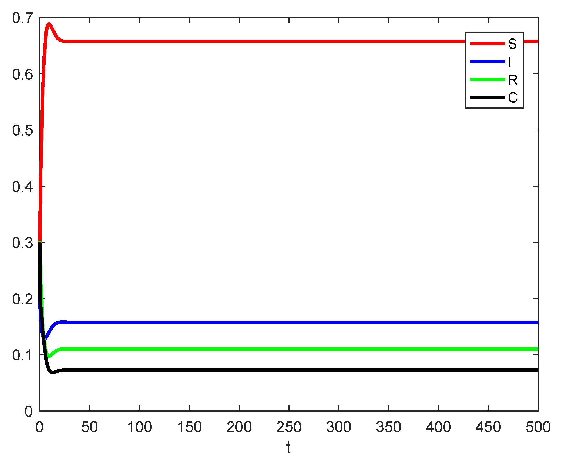
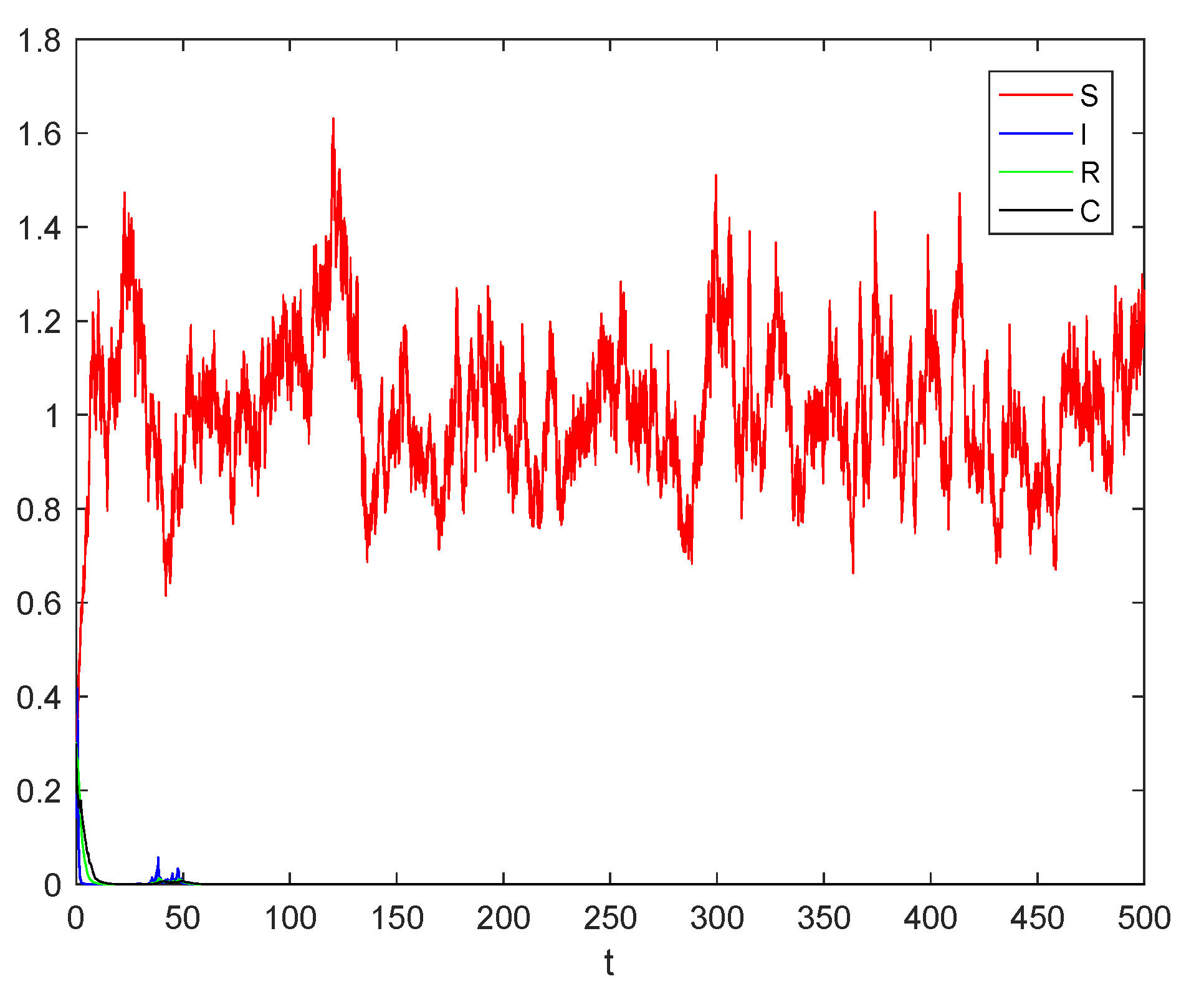
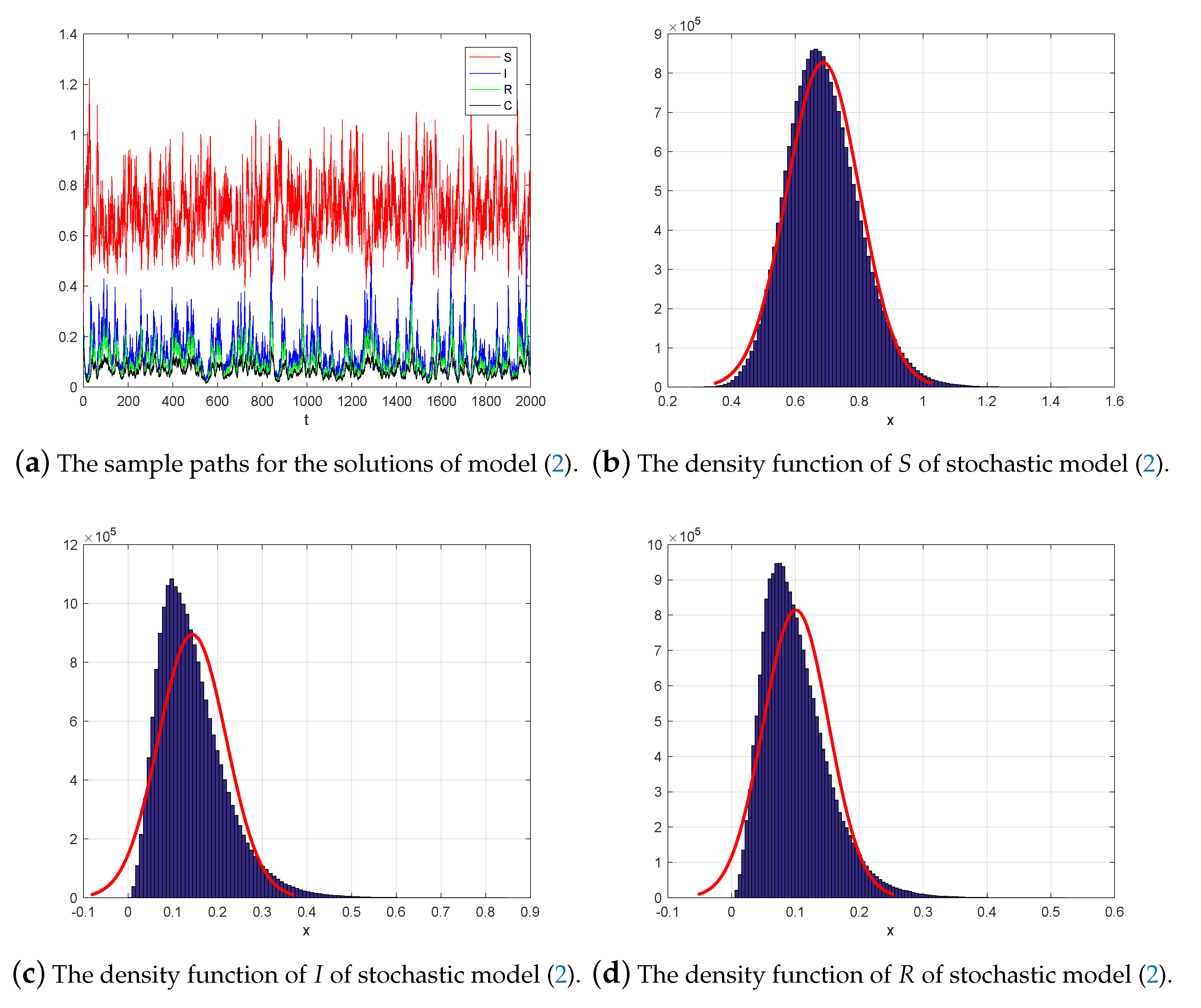
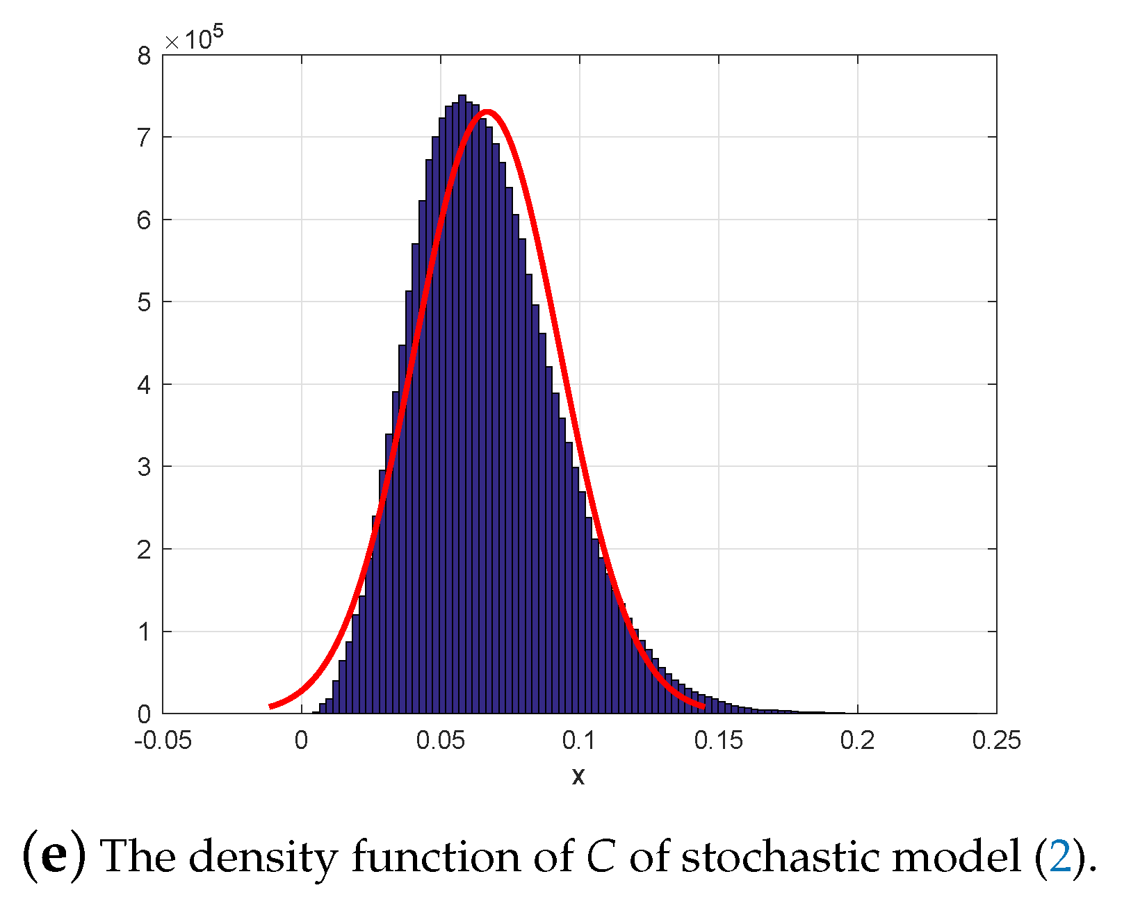
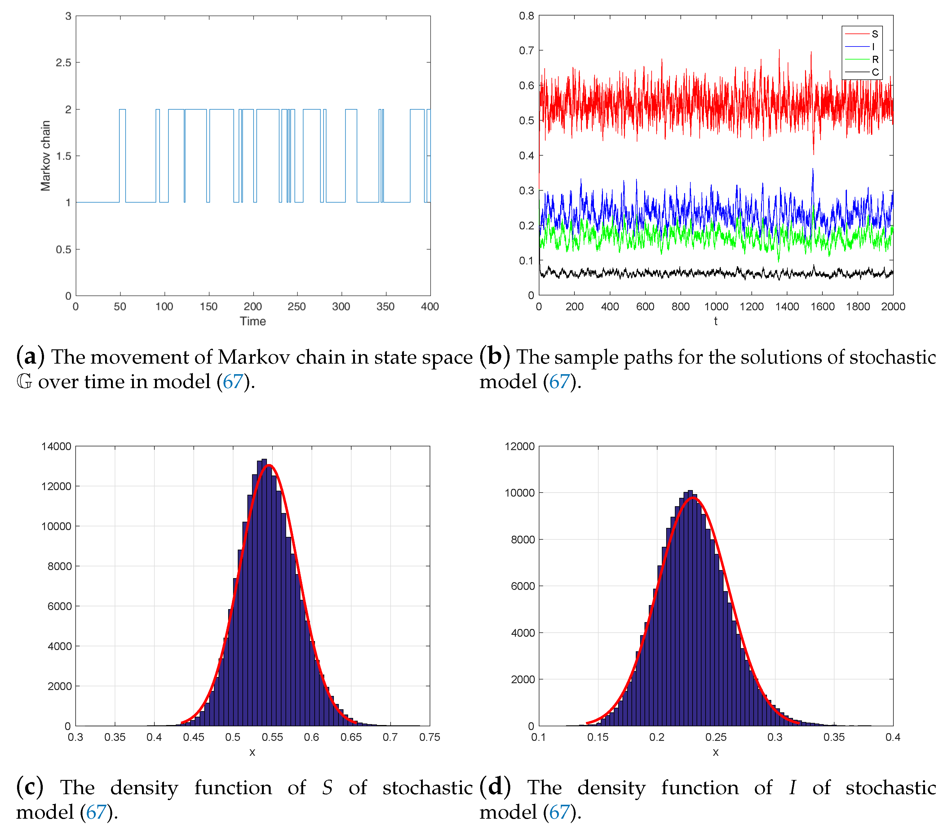
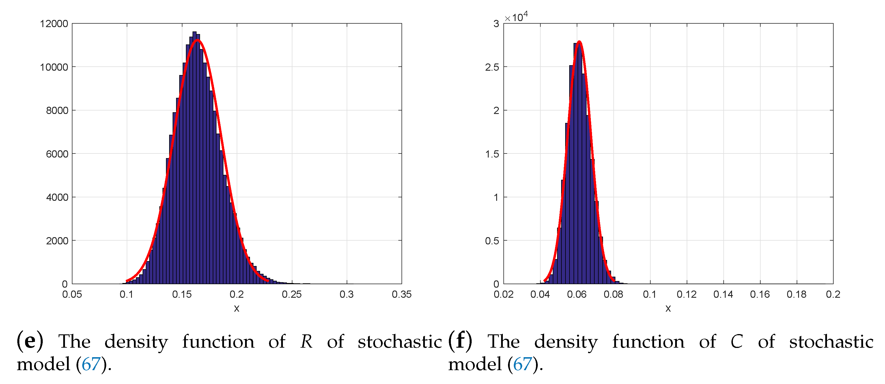
6. Numerical Simulations

In this section, we verify the theoretical results by some numerical examples. We employ the discrete system of model (2):

$$\left\{\begin{array}{cc}\hfill S_{k+1}=& S_k+\left[\mu (1-S_k)-\beta S_k{I}_k+\gamma C_k\right]\Delta t+{\sigma }_1{S}_k\Delta B_{1,k},\hfill \\ \hfill I_{k+1}=& I_k+\left[\beta S_k{I}_k+p\beta C_k{I}_k-(\mu +\alpha )I_k\right]\Delta t+{\sigma }_2{I}_k\Delta B_{2,k},\hfill \\ \hfill R_{k+1}=& R_k+\left[(1-p)\beta C_k{I}_k+\alpha I_k-(\mu +\delta )R_k\right]\Delta t+{\sigma }_3{R}_k\Delta B_{3,k},\hfill \\ \hfill C_{k+1}=& C_k+\left[\delta R_k-\beta C_k{I}_k-(\mu +\gamma )C_k\right]\Delta t+{\sigma }_4{C}_k\Delta B_{4,k},\hfill \end{array}\right.$$

(64)

where $\Delta B_{i,k}\triangleq B\left(t_{k+1}\right)-B\left(t_k\right)(i=1,2,3,4)$ obey the Gaussian distribution $N(0,\Delta t)$.

The basic parameters are taken for model (1) and model (2) as $\mu =0.2,p=0.4,\beta =0.8,\delta =0.4,\gamma =0.2,\alpha =0.35$ with $\left(S\right(0),I(0),R(0),C(0\left)\right)=(0.3,0.2,0.3,0.2).$ First, we focus on the deterministic model (1), direct calculation shows that $R_0=1.4545>1,$ then by Theorem 2.2 in Li and Guo [25], the equilibrium $E^{\ast }$ is globally asymptotically stable, which implies that the disease will eventually spread (see Figure 1).

Now, Let us consider the effect of white noise, we have the following cases to be discussed.

$\mathbf{Case}\mathbf{1}.$ Let ${\sigma }_i=0.1(i=1,3,4),{\sigma }_2=0.9,$ direct calculation shows $R_1=0.8376<1,$ it follows from Theorem 2, the disease will go to extinction eventually (see Figure 2).

$\mathbf{Case}\mathbf{2}.$ If we let ${\sigma }_i=0.1(i=1,3,4),{\sigma }_2=0.2,$ then we obtain $R_2=1.3693>1,$ according to Theorem 3, the model (2) has a unique stationary distribution, Figure 3b–e depict the probability density of the variables $S,I,R$ and $C,$ respectively, the filled contour is sample distribution and the drawn line is density function. Figure 3a is the corresponding sample paths.

7. Discussion

In present paper, we proposed and analyzed a SIRC epidemic model for Influenza A with stochastic perturbation. The effect of stochastic white noise to the SIRC epidemic is investigated. Our results show the white noise has a great impact on the elimination and spread of epidemic disease. Mathematically, on the one hand, we obtain if the threshold $R_1<1,$ then the epidemic disease will go to extinction. On the other hand, if the value $R_2>1,$ then stochastic SIRC model has a unique ergodic stationary distribution $\pi (·)$.

However, besides the effect of white noise, we also can consider the colored noise which can switch the state of the system [54,55]. Generally, this switching usually can be portrayed by a continuous-time Markov chain ${\left(\xi \left(t\right)\right)}_{t\ge 0}$ in a finite state space $\mathbb{G}=\{1,2,\dots ,N\},$ where the generator $\tilde{\mathrm{Y}}={\left({\gamma }_{ij}\right)}_{N\times N}$ can be expressed as

$$\mathbb{P}\{\xi (t+\Delta t)=j|\xi \left(t\right)=i\}=\left\{\begin{array}{c}{\gamma }_{ij}\Delta t+o(\Delta t),ifi\ne j,\hfill \\ 1+{\gamma }_{ii}\Delta t+o(\Delta t),ifi=j,\hfill \end{array}\right.$$

(65)

here $\Delta t>0,{\gamma }_{ij}\ge 0$ for $i,j=1,2,\dots ,N$ with $j\ne i$ and ${\gamma }_{ii}=-{\sum }_{j\ne i}{\gamma }_{ij}$ for each $i=1,2\dots ,N.$

If $\xi \left(t\right)$ and Brownian motions are mutually independent on $(\Omega ,\mathcal{F},{\left\{{\mathcal{F}}_t\right\}}_{t\ge 0},\mathbb{P})$ and ${\gamma }_{ij}>0$ for $i,j=1,2,\dots ,N$ with $j\ne i,$ then $\xi \left(t\right)$ is irreducible, and a unique stationary distribution $\pi =({\pi }_1,{\pi }_2,\dots ,{\pi }_N)$ of $\xi \left(t\right)$ can be determined by

$$\pi \tilde{\mathrm{Y}}=0,$$

(66)

satisfying ${\sum }_{i=1}^N{\pi }_i=1$ and ${\pi }_i>0$ for any $i\in \mathbb{G}.$

Then we get a stochastic SIRC model with regime switching as follows,

$$\left\{\begin{array}{c}{\displaystyle \mathrm{d}S\left(t\right)=\left[\mu \left(\xi \right(t\left)\right)(1-S(t\left)\right)-\beta \left(\xi \right(t\left)\right)S\left(t\right)I\left(t\right)+\gamma \left(\xi \right(t\left)\right)C\left(t\right)\right]\mathrm{d}t+{\sigma }_1\left(\xi \left(t\right)\right)S\left(t\right)\mathrm{d}{B}_1\left(t\right),}\hfill \\ {\displaystyle \mathrm{d}I\left(t\right)=\left[\beta \left(\xi \right(t\left)\right)S\left(t\right)I\left(t\right)+p\left(\xi \right(t\left)\right)\beta \left(\xi \right(t\left)\right)C\left(t\right)I\left(t\right)-\left(\mu \right(\xi \left(t\right))+\alpha (\xi \left(t\right)\left)\right)I\left(t\right)\right]\mathrm{d}t+{\sigma }_2\left(\xi \left(t\right)\right)I\left(t\right)\mathrm{d}{B}_2\left(t\right),}\hfill \\ {\displaystyle \mathrm{d}R\left(t\right)=\left[(1-p(\xi \left(t\right)\left)\right)\beta C\left(t\right)I\left(t\right)+\alpha \left(\xi \right(t\left)\right)I\left(t\right)-\left(\mu \right(\xi \left(t\right))+\delta (\xi \left(t\right)\left)\right)R\left(t\right)\right]\mathrm{d}t+{\sigma }_3\left(\xi \left(t\right)\right)R\left(t\right)\mathrm{d}{B}_3\left(t\right),}\hfill \\ {\displaystyle \mathrm{d}C\left(t\right)=\left[\delta \left(\xi \right(t\left)\right)R\left(t\right)+\beta \left(\xi \right(t\left)\right)C\left(t\right)I\left(t\right)-\left(\mu \right(\xi \left(t\right))+\gamma (\xi \left(t\right)\left)\right)C\left(t\right)\right]\mathrm{d}t+{\sigma }_4\left(\xi \left(t\right)\right)C\left(t\right)\mathrm{d}{B}_4\left(t\right),}\hfill \end{array}\right.$$

(67)

For any $k\in \mathbb{G},$$\mu \left(k\right)$, $\alpha \left(k\right)$, $\beta \left(k\right)$, $p\left(k\right)$, $\gamma \left(k\right)$, $\delta \left(k\right)$ and ${\sigma }_i\left(k\right)(i=1,2,3,4)$ are all positive constants.

Define

$$R^{\ast }=\frac{{\left[{\sum }_{k=1}^N{\pi }_k\sqrt{\mu \left(k\right)\beta \left(k\right)}\right]}^2}{{\sum }_{k=1}^N{\pi }_k\left(\mu \left(k\right)+\frac{{\sigma }_1^2\left(k\right)}{2}\right){\sum }_{k=1}^N{\pi }_k\left(\mu \left(k\right)+\alpha \left(k\right)+\frac{{\sigma }_2^2\left(k\right)}{2}\right)}.$$

(68)

Theorem 4.

If $R^{\ast }>1$ holds, the solution $(S\left(t\right),I\left(t\right),R\left(t\right),C\left(t\right),\xi \left(t\right))\in {\mathbb{R}}_{+}^4\times \mathcal{M}$ of system (67) with initial value $(S\left(0\right),I\left(0\right),R\left(0\right),C\left(0\right),\xi \left(0\right))\in {\mathbb{R}}_{+}^4\times \mathbb{G},$ produces a unique ergodic stationary distribution.

$\mathbf{Case}\mathbf{3}.$ Let $\mathbb{G}=\{1,2\}$ and the generator $\tilde{\mathrm{Y}}$ takes

$$\tilde{\mathrm{Y}}=\left(\begin{array}{cc}-0.6& 0.6\\ 0.4& -0.4\end{array}\right).$$

(69)

Then, we get the unique stationary distribution

$$\pi =({\pi }_1,{\pi }_2)=(0.4,0.6).$$

(70)

In model (67), let $\mu \left(1\right)=0.2,\alpha \left(1\right)=0.25,\beta \left(1\right)=0.8,p\left(1\right)=0.3,\delta \left(1\right)=0.2,\gamma \left(1\right)=0.15,$ $({\sigma }_1\left(1\right),{\sigma }_2\left(1\right),{\sigma }_3\left(1\right),{\sigma }_4\left(1\right))=(0.05,0.05,0.05,0.05),\mu \left(2\right)=0.3,\alpha \left(2\right)=0.3,\beta \left(2\right)=0.9,p\left(2\right)=0.3,\delta \left(2\right)=0.3,\gamma \left(2\right)=0.25,({\sigma }_1\left(2\right),{\sigma }_2\left(2\right),{\sigma }_3\left(2\right),{\sigma }_4\left(2\right))=(0.1,0.1,0.1,0.1).$ Simple calculation shows $R^{\ast }=1.5545>1,$ by Theorem 4, model (67) has a stationary distribution. In Figure 4, Figure 4a shows Markov chain and Figure 4b shows the sample paths for the solutions of stochastic SIRC model (19). Figure 4c–f show the probability density functions of $S\left(t\right)$, $I\left(t\right)$, $R\left(t\right)$ and $C\left(t\right),$ respectively, and the filled contour is sample distribution and the drawn line is density function.

References

1. Duesberg, P.H. The RNA of influenza virus. Proc. Natl. Acad. Sci. USA 1968, 59, 930–937. [Google Scholar] [CrossRef] [PubMed] [Green Version]
2. Ritchey, M.B.; Palese, P.; Kilbourne, E.D. RNAs of influenza A, B, and C viruses. J. Virol. 1976, 18, 738–744. [Google Scholar] [CrossRef] [PubMed] [Green Version]
3. Nicholson, K. Clinical features of influenza. Semin. Respir. Infect. 1992, 7, 26–37. [Google Scholar]
4. WHO. World Health Organization Report: Research for Universal Health Coverage. Technical Report, World Health Organization. Available online: http://www.who.int/whr/en/ (accessed on 1 January 2019).
5. Palese, P.; Young, J. Variation of influenza A, B, and C viruses. Science 1982, 215, 1468–1474. [Google Scholar] [CrossRef] [PubMed]
6. Hause, B.M.; Ducatez, M.; Collin, E.A.; Ran, Z.; Liu, R.; Sheng, Z.; Armien, A.; Kaplan, B.; Chakravarty, S.; Hoppe, A.D.A. Isolation of a Novel Swine Influenza Virus from Oklahoma in 2011 Which Is Distantly Related to Human Influenza C Viruses. PLoS Pathogens 2013, 9, e1003176. [Google Scholar] [CrossRef] [PubMed] [Green Version]
7. Jiang, W.M.; Wang, S.C.; Peng, C.; Yu, J.M.; Zhuang, Q.Y.; Hou, G.Y.; Liu, S.; Li, J.P.; Chen, J.M. Identification of a potential novel type of influenza virus in Bovine in China. Virus Genes 2014, 49, 493–496. [Google Scholar] [CrossRef] [PubMed]
8. Quast, M.; Sreenivasan, C.; Sexton, G.; Nedland, H.; Singrey, A.; Fawcett, L.; Miller, G.; Lauer, D.; Voss, S.; Pollock, S.; et al. Serological evidence for the presence of influenza D virus in small ruminants. Vet. Microbiol. 2015, 180, 281–285. [Google Scholar] [CrossRef] [Green Version]
9. Ducatez, M.; Pelletier, C.; Meyer, G. Influenza D Virus in Cattle, France, 2011–2014. Emerg. Infect. Dis. 2015, 21, 368–371. [Google Scholar] [CrossRef]
10. Ng, T.F.F.; Kondov, N.O.; Deng, X.; Eenennaam, A.V.; Neibergsa, H.L.; Delwart, E. A Metagenomics and Case–Control Study To Identify Viruses Associated with Bovine Respiratory Disease. J. Virol. 2015, 89, 5340–5349. [Google Scholar] [CrossRef] [Green Version]
11. Earn, D.J.; Dushoff, J.; Levin, S.A. Ecology and evolution of the flu. Trends Ecol. Evol. 2002, 17, 334–340. [Google Scholar] [CrossRef]
12. Bouvier, N.M.; Palese, P. The biology of influenza viruses. Vaccine 2008, 26, D49–D53. [Google Scholar] [CrossRef] [PubMed] [Green Version]
13. Palese, P.; Shaw, M. Orthomyxoviridae: The viruses and their replication. In Fields Virology; Knipe, D., Howley, P., Griffin, D., Lamb, R., Martin, M., Roizman, B., Strauss, E., Eds.; Lippincott Williams & Wilkins: Hiladelphia, PA, USA, 2007. [Google Scholar]
14. Feng, T.; Qiu, Z.; Meng, X. Dynamics of a stochastic hepatitis C virus system with host immunity. Discret. Contin. Dyn. Syst.-B 2019, 24, 6367–6385. [Google Scholar] [CrossRef] [Green Version]
15. Feng, T.; Qiu, Z.; Meng, X.; Rong, L. Analysis of a stochastic HIV-1 infection model with degenerate diffusion. Appl. Math. Comput. 2019, 348, 437–455. [Google Scholar] [CrossRef]
16. Feng, T.; Qiu, Z.; Meng, X. Analysis of a stochastic recovery-relapse epidemic model with periodic parameters and media coverage. J. Appl. Anal. Comput. 2019, 9, 1007–1021. [Google Scholar] [CrossRef]
17. Zhang, T.; Gao, N.; Wang, T.; Liu, H.; Jiang, Z. Global dynamics of a model for treating microorganisms in sewage by periodically adding microbial flocculants. Math. Biosci. Eng. 2020, 17, 179–201. [Google Scholar] [CrossRef]
18. Zhang, T.; Wang, J.; Li, Y.; Jiang, Z.; Han, X. Dynamics analysis of a delayed virus model with two different transmission methods and treatments. Adv. Differ. Equ. 2020, 2020, 1. [Google Scholar] [CrossRef] [Green Version]
19. Webster, R.G.; Bean, W.J.; Gorman, O.T.; Chambers, T.M.; Kawaoka, Y. Evolution and ecology of influenza A viruses. Microbiol. Mol. Biol. Rev. 1992, 56, 152–179. [Google Scholar] [CrossRef]
20. Webster, R.; Laver, W.; Air, G.; Schild, G. Molecular mechanisms of variation in influenza viruses. Nature 1982, 296, 115–121. [Google Scholar] [CrossRef]
21. Larson, H.; Tyrrell, D.; Bowker, C.; Potter, C.; Schild, G. Immunity to challenge in volunteers vaccinated with an inactivated current or earlier strain of influenza A(H3N2). J. Hyg. 1978, 80, 243–248. [Google Scholar] [CrossRef] [Green Version]
22. Davies, J.; Grilli, E.; Smith, A. Influenza A: Infection and reinfection. J. Hyg. 1984, 92, 125–127. [Google Scholar] [CrossRef] [Green Version]
23. Levine, A. Viruses; W.H. Freeman & Company: New York, NY, USA, 1992. [Google Scholar]
24. Casagrandi, R.; Bolzoni, L.; Levin, S.A.; Andreasen, V. The SIRC model and influenza A. Math. Biosci. 2006, 200, 152–169. [Google Scholar] [CrossRef] [PubMed]
25. Li, H.; Guo, S. Dynamics of a SIRC epidemiological model. Electron. J. Differ. Equ. 2017, 2017, 1–18. [Google Scholar]
26. Zhu, F.; Meng, X.; Zhang, T. Optimal harvesting of a competitive n-species stochastic model with delayed diffusions. Math. Biosci. Eng. 2019, 16, 1554–1574. [Google Scholar] [CrossRef] [PubMed]
27. Zhang, H.; Zhang, T. The stationary distribution of a microorganism flocculation model with stochastic perturbation. Appl. Math. Lett. 2020, 103, 106217. [Google Scholar] [CrossRef]
28. Liu, G.; Qi, H.; Chang, Z.; Meng, X. Asymptotic stability of a stochastic May mutualism system. Comput. Math. Appl. 2020, 79, 735–745. [Google Scholar] [CrossRef]
29. Chi, M.; Zhao, W. Dynamical analysis of two-microorganism and single nutrient stochastic chemostat model with monod-haldane response function. Complexity 2019, 2019, 8719067. [Google Scholar] [CrossRef]
30. Zhao, W.; Liu, J.; Chi, M.; Bian, F. Dynamics analysis of stochastic epidemic models with standard incidence. Adv. Differ. Equ. 2019, 2019, 22. [Google Scholar] [CrossRef] [Green Version]
31. Jiang, D.; Ji, C.; Shi, N.; Yu, J. The long time behavior of DI SIR epidemic model with stochastic perturbation. J. Math. Anal. Appl. 2010, 372, 162–180. [Google Scholar] [CrossRef] [Green Version]
32. Ji, C.; Jiang, D. Threshold behaviour of a stochastic SIR model. Appl. Math. Model. 2014, 38, 5067–5079. [Google Scholar] [CrossRef]
33. Tuckwell, H.C.; Williams, R.J. Some properties of a simple stochastic epidemic model of SIR type. Math. Biosci. 2007, 208, 76–97. [Google Scholar] [CrossRef]
34. Dieu, N.T.; Nguyen, D.H.; Du, N.H.; Yin, G. Classification of Asymptotic Behavior in a Stochastic SIR Model. SIAM J. Appl. Dyn. Syst. 2016, 15, 1062–1084. [Google Scholar] [CrossRef]
35. Miao, A.; Zhang, T.; Zhang, J.; Wang, C. Dynamics of a stochastic SIR model with both horizontal and vertical transmission. J. Appl. Anal. Comput. 2018, 8, 1108–1121. [Google Scholar]
36. Beretta, E.; Kolmanovskii, V.; Shaikhet, L. Stability of epidemic model with time delays influenced by stochastic perturbations. Math. Comput. Simul. 1998, 45, 269–277. [Google Scholar] [CrossRef]
37. Bacaër, N. On the stochastic SIS epidemic model in a periodic environment. J. Math. Biol. 2014, 71, 491–511. [Google Scholar] [CrossRef] [PubMed] [Green Version]
38. Gray, A.; Greenhalgh, D.; Mao, X.; Pan, J. The SIS epidemic model with Markovian switching. J. Math. Anal. Appl. 2012, 394, 496–516. [Google Scholar] [CrossRef] [Green Version]
39. Cai, Y.; Kang, Y.; Banerjee, M.; Wang, W. A stochastic epidemic model incorporating media coverage. Commun. Math. Sci. 2016, 14, 893–910. [Google Scholar] [CrossRef]
40. Gao, N.; Song, Y.; Wang, X.; Liu, J. Dynamics of a stochastic SIS epidemic model with nonlinear incidence rates. Adv. Differ. Equ. 2019, 2019, 41. [Google Scholar] [CrossRef] [Green Version]
41. Zhao, Y.; Zhang, L.; Yuan, S. The effect of media coverage on threshold dynamics for a stochastic SIS epidemic model. Phys. A Stat. Mech. Appl. 2018, 512, 248–260. [Google Scholar] [CrossRef]
42. Zhou, Y.; Yuan, S.; Zhao, D. Threshold behavior of a stochastic SIS model with jumps. Appl. Math. Comput. 2016, 275, 255–267. [Google Scholar]
43. Song, Y.; Miao, A.; Zhang, T.; Wang, X.; Liu, J. Extinction and persistence of a stochastic SIRS epidemic model with saturated incidence rate and transfer from infectious to susceptible. Adv. Differ. Equ. 2018, 2018, 293. [Google Scholar] [CrossRef] [Green Version]
44. Lahrouz, A.; Settati, A. Qualitative Study of a Nonlinear Stochastic SIRS Epidemic System. Stoch. Anal. Appl. 2014, 32, 992–1008. [Google Scholar] [CrossRef]
45. Liu, Q.; Jiang, D.; Shi, N.; Hayat, T.; Alsaedi, A. Stationary distribution and extinction of a stochastic SIRS epidemic model with standard incidence. Phys. A Stat. Mech. Appl. 2017, 469, 510–517. [Google Scholar] [CrossRef]
46. Liu, M.; Bai, C.; Wang, K. Asymptotic stability of a two-group stochastic SEIR model with infinite delays. Commun. Nonlinear Sci. Numer. Simul. 2014, 19, 3444–3453. [Google Scholar] [CrossRef]
47. Mao, X. Stochastic Differential Equations and Applications, 2nd ed.; Horwood Publishing: Chichester, UK, 2007. [Google Scholar]
48. Khasminskii, R. Stochastic Stability of Differential Equations, 2nd ed.; Springer-Verlag: Berlin/Heidelberg, Germany, 2012; Volume 66. [Google Scholar]
49. Li, F.; Zhang, S.; Meng, X. Dynamics analysis and numerical simulations of a delayed stochastic epidemic model subject to a general response function. Comput. Appl. Math. 2019, 38, 95. [Google Scholar] [CrossRef]
50. Mao, X.; Marion, G.; Renshaw, E. Environmental Brownian noise suppresses explosions in population dynamics. Stoch. Proces. Appl. 2002, 97, 95–110. [Google Scholar] [CrossRef]
51. Liptser, R. A strong law of large numbers for local martingales. Stochastics 1980, 3, 217–228. [Google Scholar] [CrossRef]
52. Gard, T.C. Introduction to Stochastic Differential Equations(Pure and Applied Mathematics); Marcel Dekker Inc.: New York, NY, USA, 1988. [Google Scholar]
53. Zhu, C.; Yin, G. Asymptotic Properties of Hybrid Diffusion Systems. SIAM J. Control Optim. 2007, 46, 1155–1179. [Google Scholar] [CrossRef]
54. Gao, M.; Jiang, D. Ergodic stationary distribution of a stochastic chemostat model with regime switching. Phys. A Stat. Mech. Appl. 2019, 524, 491–502. [Google Scholar] [CrossRef]
55. Settati, A.; Lahrouz, A. Stationary distribution of stochastic population systems under regime switching. Appl. Math. Comput. 2014, 244, 235–243. [Google Scholar] [CrossRef]
Figure 1. Time series of S , I , C , R for model (1), the epidemic disease is persistent.
Symmetry 12 00745 g001
Figure 2. Time series of S , I , C , R for the stochastic model, where σ i = 0.1 ( i = 1 , 3 , 4 ) , σ 2 = 0.9 , the epidemic disease goes to extinction.
Symmetry 12 00745 g002
Figure 3. Basic behavior of solutions for stochastic model where σ i = 0.1 ( i = 1 , 3 , 4 ) , σ 2 = 0.2 .
Symmetry 12 00745 g003aSymmetry 12 00745 g003b
Figure 4. Illustration of basic behavior of solutions of stochastic model where σ i = 0.1 ( i = 1 , 3 , 4 ) , σ 2 = 0.2 .
Symmetry 12 00745 g004aSymmetry 12 00745 g004b