What Experts Appreciate in Patterns: Art Expertise Modulates Preference for Asymmetric and Face-Like Patterns

Abstract

This study set out to investigate whether and how aesthetic evaluations of different types of symmetric, as well as abstract vs. representational patterns are modulated by art expertise. To this end, we utilized abstract asymmetric, symmetric, and “broken” patterns slightly deviating from symmetry, as well as more representational patterns resembling faces (also symmetric or broken). While it has already been shown that symmetry preference decreases with art expertise, it was still unclear whether an already established relationship between art expertise and preference for abstract over representational art can be similarly found as a preference for abstract over representational patterns, as these are non-art objects. Nevertheless, we found profound differences in aesthetic preferences between art experts and laypersons. While art experts rated asymmetric patterns higher than laypersons, as expected, they rated face-like patterns lower than laypersons. Also, laypersons rated all other types of patterns higher than asymmetric patterns, while art experts rated the other patterns similar or lower than asymmetric patterns. We found this both for liking and for interest ratings. As no differences between art experts and laypersons were found regarding memory recognition of new and old patterns, this effect is not likely due to differences in memory performance. In sum, this study further extends our knowledge about the influence of art expertise on aesthetic appreciation.

1. Introduction

Symmetry is an important—if not the most important—predictor of aesthetic evaluation for many types of images. It can be found everywhere [1,2,3] and it is often considered to be relevant for the beauty of an object [4,5,6,7,8,9]. Symmetry is also one of the classical Gestalt principles that enable perceptual grouping and determine “good shape” [10,11]. Symmetry can be rapidly detected—especially if it is vertical (bilateral) symmetry [2,3,12,13,14,15]. On the other hand, symmetry has a rather low standing in art, where it is considered to be at best one of many other factors influencing aesthetic evaluation. Also, it has been assumed that preference for symmetry decreases with art training [16,17,18,19]. However, symmetry is clearly especially relevant for the aesthetics of abstract patterns [7,20,21,22,23,24,25,26,27,28,29,30,31] and human faces [32,33,34,35,36,37,38,39].

Many researchers claimed that symmetry is the most important predictor of aesthetic evaluation in abstract patterns [7,21,22,23,25,27,30,31,40]. Though, concerning the aesthetic appeal of small differences to perfect symmetry, results are somewhat mixed. McManus [17] argued that while symmetry is often linked to beauty, it can also be perceived as sterile and rigid. Consequently, deviations from symmetry are relatively common in art. Specifically, he found that almost 30% of the investigated polyptychs from the Italian Renaissance contain a form of deliberately broken, thus imperfect, symmetry. While this does not necessarily mean that such deviations from symmetry increased aesthetic appeal, and they probably also had some symbolic meanings, McManus concludes from this and other examples that some asymmetry can generate interest and excitement in artworks. For abstract patterns, results are also not entirely clear. While some researchers found that small deviations from symmetry are not liked [27], others found—using an unusual gaze-driven evolutionary algorithm to make participants produce instead of only evaluate stimuli—that small differences from perfect symmetry can be at least tolerated [41]. It seems likely that these mixed findings are the result of different types of applied stimuli and/or evaluation (respectively production) methods. The human face is a special case of a symmetric object, whose evaluations of beauty and attractiveness are thought to be deeply rooted in biology and evolutionary factors. Symmetry preference in human faces is a complex process, which has been explained in different ways. First, symmetry can be interpreted as a biological signal for good genes and good health [42,43,44]. Second, symmetry preference could also simply be a by-product of efficient object recognition processes [45]—i.e., fluent processing [46,47,48]. However, some researchers [49] found a gender difference in symmetry preference for neutral stimuli and concluded that perceptual efficiency is probably not enough to explain preference for symmetry in objects. Also, there is some evidence that natural, slightly asymmetric faces might be preferred over (artificial) perfectly symmetric faces [50,51,52]. However, these two different explanations are not necessarily in conflict and might be both valid [38] and could both be interpreted as biological explanations of symmetry preference in general.

Symmetry is also linked to the concept of complexity as symmetry is a form of order and redundancy that is thought to reduce perceived complexity [19,28,46,53,54] and thus it can also be seen as an aspect of visual complexity. There is still some debate about the influence of complexity on aesthetic evaluation. While Berlyne [55,56] suggested a relationship between complexity and pleasingness in the form of an inverted U-shape (thus, medium complexity is preferred), recent research questioned the generality of this assumption [21,53,57]. The actual relationship between complexity and preference likely depends on type of used images, range of complexity, individual differences, etc. Furthermore, art training might also alter the influence of complexity on aesthetic processing [58]. However, in this paper we will not focus on the influence of visual complexity on aesthetic evaluation and therefore applied stimuli that were matched in terms of perceived visual complexity.

Another important factor that is known to influence aesthetic evaluation is art expertise—thus, an attribute of the participants (or viewers) and not the stimuli (or artworks/images). Aesthetic processing differs between laypersons and art experts [5,6,19,58,59,60,61]. For instance, following the assumptions of the model of aesthetic appreciation and aesthetic judgments [5,6], it can be assumed that higher stages of aesthetic processing like cognitive mastering are only reached by art experts [62]. Furthermore, it was found that art expertise even modulates neural activity during aesthetic judgments [63]. Specifically, experts have domain-specific knowledge and interpret artworks more in relation to artistic style, while laypersons do refer more to personal experiences and feelings [64]. Also, art experts often rate artworks higher than art novices. More differences between art experts and novices were found in cognition-oriented judgments such as beauty and liking, than in affective judgments as valence and arousal [65]. While emotions play an important role for art appreciation in general, non-experts show higher correlations between emotions and understanding than experts [66]. In contrast, art experts show attenuated reactions to emotionally-valenced art [67]. Furthermore, experts often find art more interesting and easier to understand (or less confusing). This is particularly the case regarding abstract or complex art [58,68]. Interestingly, degrading of art images (from figurative to abstract or from color to black-and-white) seems to have a stronger negative effect on laypersons than on experts. Thus, artistic taste appears to change with artistic training [69]. Also, it was found that level of abstractness of paintings influences the aesthetic judgments and emotional valence of laypersons but not of experts. Laypersons’ aesthetic and emotional ratings were highest for representational and lowest for abstract paintings, while experts were independent of abstraction level [70]. These results were also confirmed in a recent study [71] that found that experts rated abstract artworks as more interesting and more beautiful than representational artworks. While non-experts strongly distinguished between abstract and representational artworks, experts appraised these two types of art similarly. Also, it has been suggested that symmetry preference decreases with art training [16,18,19]. Thus, level of abstraction, and to a lesser extent also symmetry, seem to be important properties of artworks, which are differently processed by art experts and laypersons.

In the present study, we use abstract black-and-white patterns as stimuli, similar to those applied by Gartus and Leder [27,28]. While symmetry is a known strong predictor of aesthetic appreciation, it can be assumed that symmetry preference also differs between art experts and laypersons [17,19]. A recent study [18] directly compared preference for symmetry in art experts and laypersons. Consistent with many previous studies, it was found that symmetrical patterns were generally preferred over asymmetrical patterns. Also, using implicit evaluation (Implicit Association Test, IAT), no difference in preference for symmetrical over asymmetrical patterns was found in art experts vs. laypersons. However, when asked to rate the patterns explicitly, beauty ratings increased for asymmetrical patterns in experts, while they still rated symmetrical patterns higher than asymmetrical patterns. Another recent study [16] employing only explicit beauty ratings even found complete contrasting preferences between art experts and laypersons; experts did prefer asymmetric over symmetric patterns, while it was the complete opposite for laypersons.

So, what makes the difference between an art expert and a layperson regarding aesthetic preferences? While some of the differences involve the interplay of cognitive and emotional processing [67], we also assume another distinction that is more related to visual and contextual processing. For instance, some authors [72] suggested that the aesthetic preferences of laypersons evolved from direct natural selection, while the aesthetic preferences of art experts are also indirectly selected via an ongoing process of coevolution based on prestige-driven social learning. Thus, experts’ appreciation of artworks is more based on the prestige of the associated context and the admiration of the artist. This obviously requires some knowledge, which is acquired during the intense study of art and art history. That could explain why modern art (that does not always appeal to the senses as more traditional or popular art) is more likely to be appreciated by art experts, while laypersons are more attracted by what is sometimes called “easy beauty” [73]. Now, as has been discussed above, our visual system has a preference for mirror (bilateral) symmetry [3]. Thus, symmetry could possibly be interpreted as a form of naturally evolved “easy beauty”, which is less appreciated by art experts. Furthermore, it is known that laypersons prefer representational over abstract art [70] and vice versa [71]. In the same way as for symmetry, one could argue that our brain and visual system evolved to rapidly recognize the gist of a visual scene [74,75] and thus, again, representational art could be interpreted as a form of more “easy beauty” compared to abstract art.

Because of the discussed importance of level of abstraction in aesthetic evaluation, we wanted to not just use abstract patterns, but also include more representational patterns in this study. To this end, we employed similar “abstract” patterns as used in Gartus and Leder [27,28]. However, already during the generation of these patterns, we had observed that a surprisingly large number of patterns having vertical (bilateral) symmetry could be perceived as (human or animal) faces. While in our previous studies, we have excluded such “faces” precisely for the fact that they are no longer abstract patterns in the full sense of the word (i.e., they do represent objects of the real world—namely faces), in the present study, we deliberately included them in our set of stimuli. Thus, the main factors we investigated in this study are the stimulus-dependent factors of level of abstractness (or “face-likeness”) and degree of symmetry, plus the participant-dependent factor of art expertise. In addition to fully symmetric and asymmetric patterns, we also included stimuli that only deviated slightly from full symmetry (“broken” symmetric patterns), as this factor showed a strong influence on aesthetic evaluation and perceived visual complexity in previous studies [27,28].

During the experiment, we also applied a mood questionnaire [76] and a questionnaire measuring need for cognitive closure [77] to be able to control for these two factors. We assumed that positive mood would generally increase the ratings and need for closure would increase ratings specifically for symmetry as it also is related to preference for order. Furthermore, an art expertise questionnaire [78] was administered to obtain an objective measure of art expertise as a major factor in our study.

In sum, the main hypotheses for the present study are that symmetry is generally preferred over asymmetry (or broken symmetry), but that this effect should be less pronounced (or even reversed) for art experts. Also, representational (“face-like”) patterns should be rated higher by laypersons than by art experts, because laypersons prefer representational over abstract artworks. We expected these hypothesized response patterns for both applied rating scales of liking and interest. Furthermore, art experts may have developed sophisticated encoding schemes during their extensive training that might potentially change their cognitive processing of visual patterns and as well help to improve memory performance. To rule out such cognitive processing differences between art experts and laypersons, which potentially could explain differences in aesthetic evaluation, we also added a memory recognition task using newly and previously presented patterns as a second part to our experiment. In addition, we also wanted to explore whether some specific stimulus types (e.g., face-like patterns) are in general easier to remember than others.

2. Materials and Methods

2.1. Stimuli

The employed stimuli were similar to those used in Gartus and Leder [27,28]. They consisted of 36 to 44 black triangles, placed in an 8 × 8 regular grid on a white background showing several types of symmetry and were generated by a stochastic optimization algorithm implemented in MATLAB R2013a (The MathWorks, Inc., Natick, MA, USA). In this study, asymmetric patterns and patterns having a vertical symmetry axis were used. In addition, we also used “broken” patterns that slightly deviated from perfect vertical symmetry [27,28]. Patterns with a vertical symmetry axis are quite often perceived as faces (the pareidolia phenomenon). To systematically study this phenomenon, 300 preselected patterns with a vertical symmetry axis were examined in three prestudies to select the stimuli for the main study.

In Prestudy 1, patterns which are either frequently or rarely perceived as faces were collected. Ten people participated in this prestudy (4 men, 6 women, age range = 25–31; mean age = 27.8; all students of psychology at the University of Vienna). Participants had to state whether they see a face in a pattern or not. As a result, 217 patterns were selected: 115 patterns that were frequently perceived as faces and 102 that were only rarely or never perceived as faces.

In Prestudy 2, we additionally collected ratings of the easiness of perceiving a face in a pattern for each of the 217 patterns selected in Prestudy 1 on a 7-point scale. Ten people participated in this prestudy (4 men, 6 women, age range = 25–37; mean age = 29.9; all students of psychology at the University of Vienna). As the combined result of Prestudy 1 and Prestudy 2, 116 patterns with a vertical symmetry axis were selected for the main study: 60 patterns often and easily perceived as faces and 56 patterns seldom or never perceived as faces.

In Prestudy 3, ratings of subjective visual complexity were collected on 7-point scales to be able to control the finally selected stimuli for complexity. Twenty-one people participated in this prestudy (9 men, 12 women, age range = 19–37; mean age = 27.2; all students at the University of Vienna) and rated 305 patterns for visual complexity.

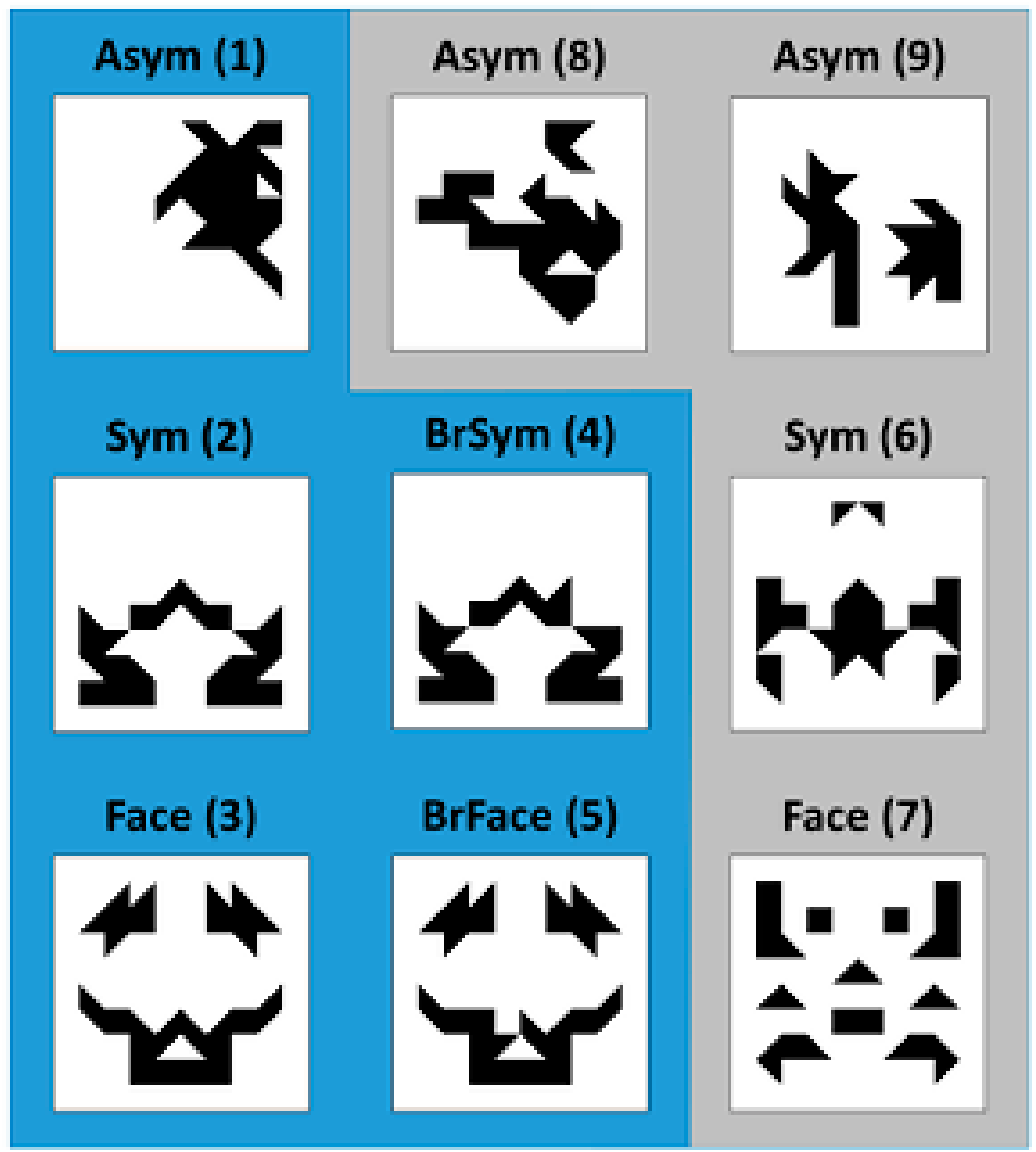
The resulting patterns were divided into five categories: Asymmetric (Asym), symmetric (Sym), symmetric face-like (Face), broken symmetric (BrSym), and broken symmetric face-like (BrFace) patterns. According to the collected mean complexity ratings, 135 patterns were selected for the main study: 90 for the first part where patterns were to be rated for liking and interest and 45 for the second part which involved a memory task. Specifically, we first selected 10 patterns from each of the categories Asym, Sym, and Face with similar mean complexity per group, as well as the corresponding patterns from the categories BrSym and BrFace (groups 1–5). Because the broken symmetric patterns showed a higher average visual complexity than the symmetric ones, we additionally selected patterns from the categories Sym, Face, and Asym (groups 6–9), matched in complexity to the selected patterns from the categories BrSym and BrFace (groups 4 and 5). In sum, we selected nine groups of patterns, each consisting of 10 patterns. See

Table 1. List of pattern groups and categories used in the main study. The last column denotes the matches between groups regarding mean visual complexity.

Pattern Group	Pattern Category	Mean Complexity (SD)	Matched to Group
1	Asym	3.55 (0.56)	2 and 3
2	Sym	3.55 (0.56)	1 and 3
3	Face	3.55 (0.56)	1 and 2
4	BrSym	4.01 (0.58)	6 and 8
5	BrFace	3.81 (0.70)	7 and 9
6	Sym	3.99 (0.52)	4 and 8
7	Face	3.80 (0.68)	5 and 9
8	Asym	4.00 (0.57)	4 and 6
9	Asym	3.84 (0.69)	5 and 7

for an overview of selected pattern groups and categories and Figure 1 for examples of selected stimulus patterns.

While for Prestudy 1 and Prestudy 2, E-Prime 2.0.8.90 (Psychology Software Tools, Inc., Pittsburgh, PA, USA) was used as experimental software, Prestudy 3 was programmed in OpenSesame 2.8.2 [79].

2.2. Participants

Mostly psychology and art history students of the University of Vienna participated in the main study. Psychology students participated for course credit, while art history students received chocolate as small thank-you in the first round of data collection and €10 in the second round, when recruiting was more difficult. In sum, 85 persons (20 men, 65 women, mean age = 25.0, SD = 5.6; 32 students or graduates of art history) participated in the study. Data collection was performed at two different time points (64 participants in 2015 and additional 21 participants in 2019). The additional testing was mostly done to increase the number of art experts in the sample (13 out of the 21 new participants). All were tested for visual acuity and gave written informed consent prior to the study. They were informed that they could quit the study at any time without further consequences. The study lasted about 30–40 min and was not in any way harmful or medically invasive. Thus, no ethical approval was requested, which is in accordance with the ethical guidelines of the University of Vienna. All but five participants were fluent German speakers.

2.3. Questionnaires

The German version of the PANAS—Positive and Negative Affect Schedule [76,80]—was applied to obtain a short measure of current mood of the participants. This was considered relevant, as it is assumed that affective states can influence cognitive processing and also the quality of aesthetic experiences [5,81,82].

In addition, we also applied a scale of need for cognitive closure (NCC; [83]). The need for cognitive closure can be defined as the desire for fast answers and predictability, as well as the preference for order and structure and discomfort with ambiguity. Thus, high need for cognitive closure could potentially lead to higher preference for symmetry and/or concrete images, in contrast to abstract images (both because of discomfort with ambiguity and faster processing due to increased fluency; [46,47]). To be able to also adjust for this factor, we used the German 16-NCCS scale [77].

As final questionnaire, an art interest and art knowledge questionnaire was employed to obtain a measure of art expertise, as this is the main between-subject factor of interest in our study. Specifically, we used a predecessor version of the VAIAK—Vienna Art Interest and Art Knowledge Questionnaire [78]—which was regularly used in our lab at the time of the study. It was assumed that art experts would be less inclined to give pareidolian faces a high rating, as they might consider them as a form of “easy beauty” [73].

Note that during the first part of data collection in 2015, questionnaires were presented online, while during the second part in 2019, paper–pencil versions of the questionnaires were used.

2.4. Experimental Procedure

The experiment was conducted on lab computers using E-Prime 2.0.8.90 in 2015 and E-Prime 2.0.10.356 (Psychology Software Tools, Inc., Pittsburgh, PA, USA) in 2019 as experimental software. Patterns were presented in a size of 500 × 500 pixels in front of a black background for 3000 ms on a variety of different monitors. Participants were sitting in an approximate distance of 70 cm to the monitors. As we did not assume an influence of small differences in presentation size, we did not control for monitor sizes.

Concerning the experimental sequence, participants were first welcomed to the experiment and asked whether they speak German proficiently. If not, we provided them all materials translated into English. Then, they filled out the informed consent form, the 16-NCCS, and the PANAS. After completion of the questionnaires, they were introduced to the first part of the experiment. Instructions were both given on the computer screen and as a short verbal summary. The task in this part of the experiment was to rate 90 abstract patterns for liking and interest on 7-point scales. The exact rating questions were: “How do you like this pattern?” (German: “Wie gefällt Ihnen dieses Muster?”) and “How interesting does this pattern appear?” (German: “Wie interessant erscheint dieses Muster?”). During the self-paced rating, small versions of the patterns (downsized to 200 × 200 pixels) were presented together with the rating scales. After finishing the first experimental part, they were given the art interest and art knowledge questionnaire. Thereafter, participants were introduced to the second part of the experiment. Here, participants were presented 90 patterns of which they had already seen 45 in the first part. Participants were asked whether they had already seen the patterns or not. The detailed question was “Have you already seen this pattern? Yes/No” (German: “Haben Sie dieses Muster bereits gesehen? Ja/Nein”). Finally, participants were debriefed. They were asked whether they recognized anything during the experiment that they want to tell us, received a short verbal explanation of the purpose of the study, and were thanked for participating.

2.5. Data Analysis

We used Bayesian linear mixed-effects models for data analysis of our experiments for several reasons; linear mixed-effects models enable generalization across stimuli and participants and not only across participants [84]. Bayesian data analysis was applied to avoid the statistical peculiarities of null-hypothesis significance testing, for instance, the dependence on predefined sampling plans [85,86,87]. More specifically, we applied Bayesian estimation and did not use Bayes Factors [88,89]. We used R version 3.6.2 [90], the tidyverse package version 1.2.1 [91] for data preparation, and the brms package version 2.10.0 [92,93], a high-level interface to Stan [94], for data analysis. We set weakly informative priors for the intercept as normal(0,5), for fixed effects as normal(0,3), and otherwise kept default priors. For model estimation, four chains with 10,000 iterations (5000 warmup and 5000 sampling) were used. Convergence was checked via Gelman–Rubin [95] convergence statistics (Rhat close or equal to 1.0) and by visual inspection of trace plots. Categorical predictors were dummy coded and continuous predictors standardized by subtracting the mean and dividing by two standard deviations [96]. The random-effects structure of the models consisted of by-subject random intercepts and random slopes of pattern category and visual complexity, and by-stimulus random intercepts and random slopes of positive and negative affect (PANAS), need for cognitive closure (16-NCCS), and art expertise (experts vs. laypersons or VAIAK). Random slopes also included all possible interactions of predictors. In the main text, traditional models are presented that treat the dependent rating variables as metric. However, because it has been shown that this can cause problems in some cases [97,98], we also included ordered-probit models in an Appendix C. Post-hoc contrasts were extracted using the emmeans package version 1.4.3.01 [99] and the tidybayes package version 1.1.0 [100]. In addition, ggplot2 package version 3.2.1 [101] was used for data visualization. The BayesianFirstAid package version 0.1 [102] was used with default settings to test correlations and to compare scores between laypersons and experts (with a Bayesian two sample test as an alternative to a t-test). All presented credible intervals are highest density intervals (HDI). We applied a decision rule based on the HDI and predefined regions of practical equivalence (ROPE) around zero [88]. For correlations, [−0.05, 0.05] was chosen as ROPE, which corresponds to half of the value of a negligible correlation following Cohen’s (1988) rule of thumb. For the linear mixed-effects models, we also chose [−0.05, 0.05] as ROPE, because predictors are standardized by dividing by two standard deviations [96]. Therefore, the resulting standard deviation is 0.5 and not 1.0 and thus, the recommended ROPE of [−0.1 * SD, 0.1 * SD] amounts to [−0.05, 0.05]. For the Bayesian t-tests, a similar rule was used as for the linear models.

3. Results

3.1. Questionnaires

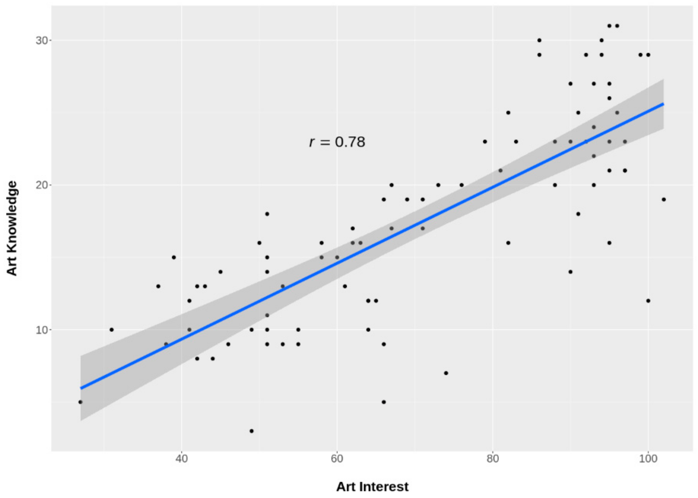
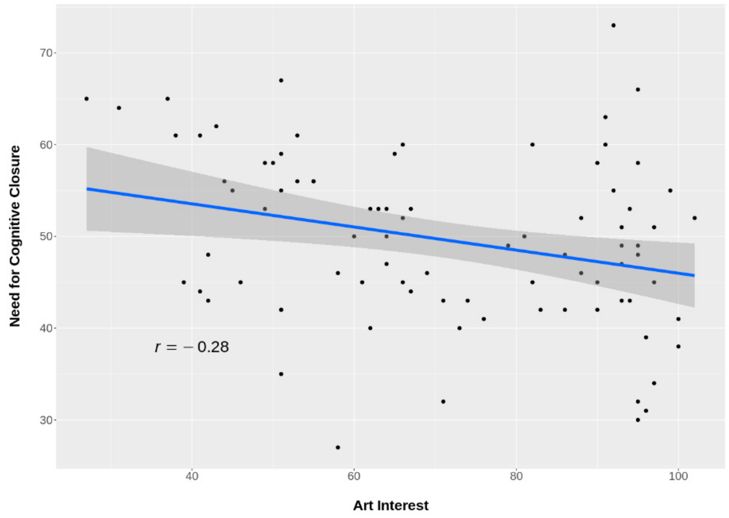
The following correlations of questionnaire scales were observed in the whole sample of the 85 participants. The two scales of the VAIAK, art interest and art knowledge, showed a strong positive correlation of r = 0.78, 95% HDI [0.69, 0.86]. See Figure A1 in Appendix A for a scatter plot. In contrast to this, need for cognitive closure (NCC) was moderately negatively correlated with art interest (r = −0.28, 95% HDI [−0.48, −0.083]) and also with art knowledge (r = −0.27, 95% HDI [−0.47, −0.072]). See Figure A2 and Figure A3 for scatter plots. Only low correlations could be observed with the PANAS scales (positive vs. negative affect: r = 0.10, 95% HDI [ −0. 13, 0.32]; NCC vs. positive affect: r = 0.01, 95% HDI [−0.22, 0.23]; NCC vs. negative affect: r = −0.17, 95% HDI [−0.34, 0.12]; art interest vs. negative affect: r = 0.05, 95% HDI [−0.18, 0.25]; art knowledge vs. negative affect: r = 0.07, 95% HDI [−0.19, 0.26]). Exceptions are the moderate positive correlations of art interest and positive affect (r = 0.31, 95% HDI [0.099, 0.49]) and art knowledge and positive affect (r = 0.17, 95% HDI [−0.051, 0.37]).

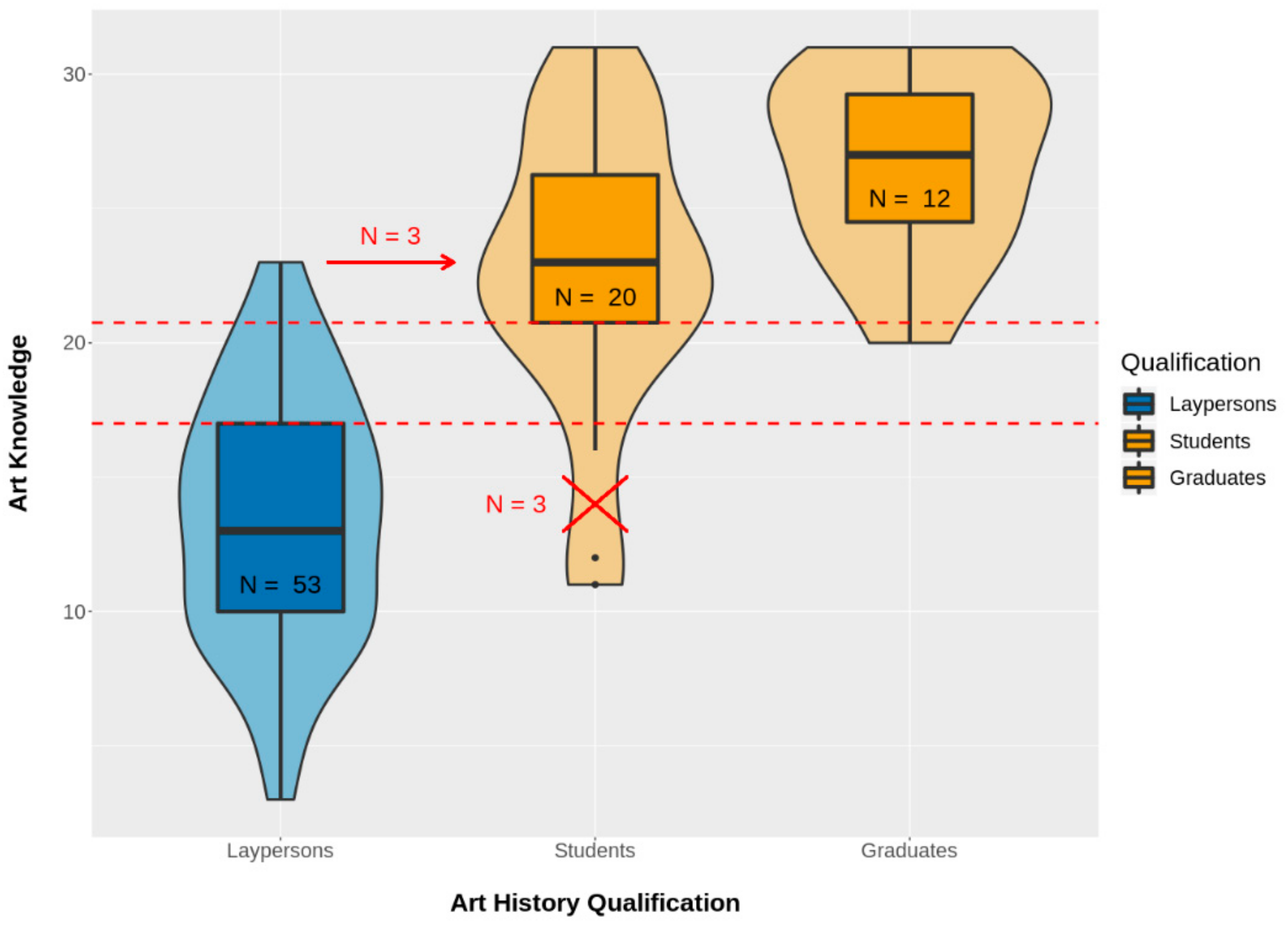
Of the 85 participants, 20 indicated in the VAIAK that they study art history, and 12 indicated that they have graduated in art history. The remaining 53 were initially considered to be art laypersons. See Figure 2 for box plots of art knowledge scores for these three groups. However, it was found that the art knowledge scores of three students of art history were so low that they fell into the interquartile range of the laypersons. These three art history students were excluded from further analysis, because art experts are expected to have a high level of art knowledge. In contrast, the art knowledge scores of three laypersons were so high that they fell into the interquartile range of art history students. These three laypersons were put into the group of art experts, because their level of art knowledge was comparable to art history students. Furthermore, one participant from the group of laypersons showed low visual acuity and was excluded from analysis. In sum, there were 81 remaining participants of which 32 were assigned to the group of art experts, and 49 to the group of laypersons.

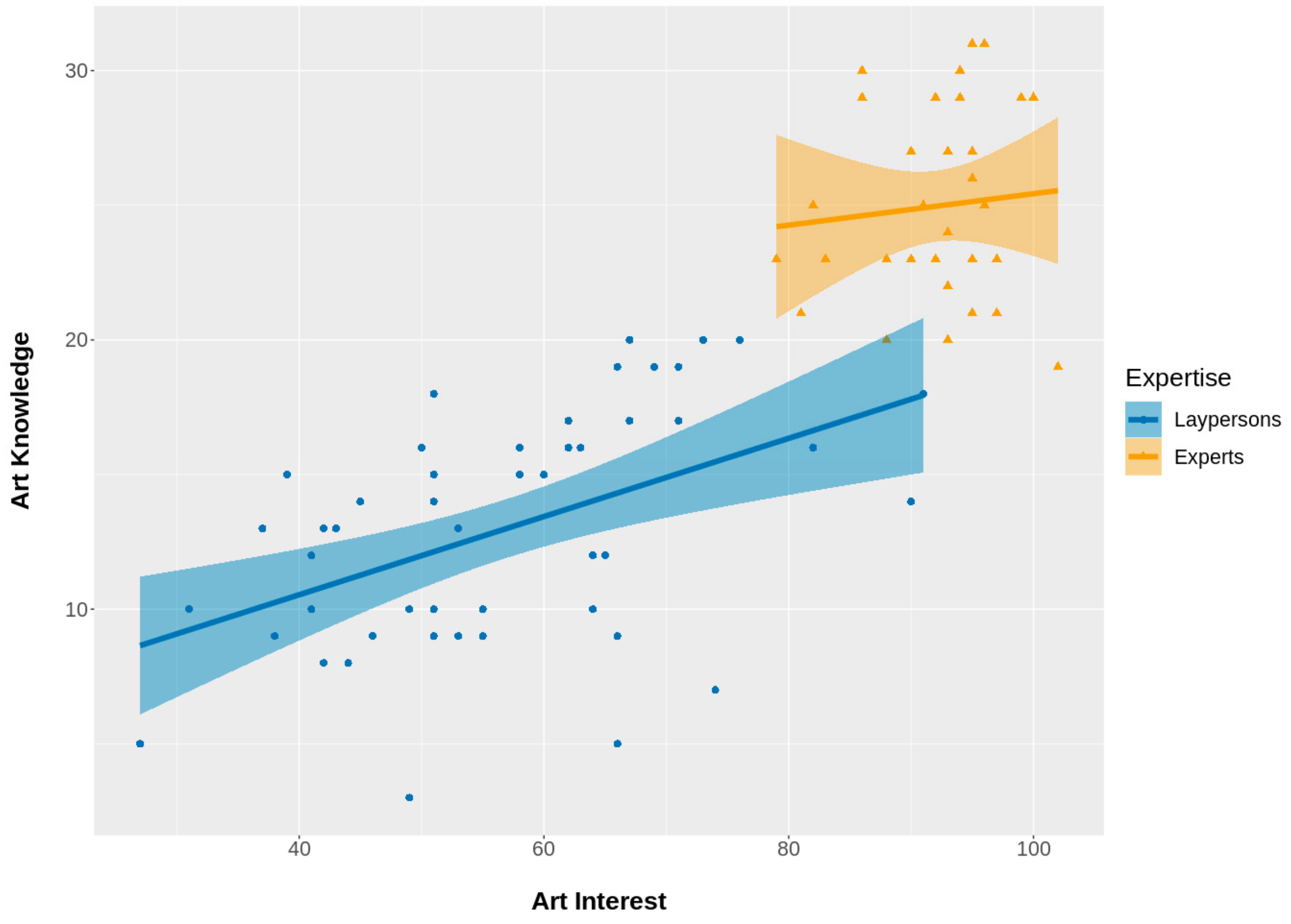
For the 81 participants (18 men, 63 women; 49 laypersons, 32 art experts, mean age = 24.6, SD = 3.5) remaining in the sample, questionnaire scores were as follows. In addition to the raw scores, we also report 95% credible intervals for the difference of the scores. The PANAS score of positive affect showed a mean of 29.8 (SD = 5.2) for laypersons and 34.0 (SD = 5.9) for art experts (difference: 95% HDI [1.5, 6.8]). Mean negative affect was 12.9 (SD = 3.3) for laypersons and 12.7 (SD = 3.5) for experts (difference: 95% HDI [−1.6, 0.74]). Since PANAS scores range from 10 to 50, it can be summarized that positive affect was on a mid-level and (slightly) higher for art experts than for laypersons, while negative affect was generally very low. Concerning need for cognitive closure (NCC), mean scores of 16-NCCS were 50.6 (SD = 9.1) for laypersons and 48.2 (SD = 9.7) for art experts (difference: 95% HDI [−6.9, 1.9]). Finally, mean VAIAK scores of art interest were 56.8 (SD = 14.2) for laypersons and 92.1 (SD = 5.57) for experts (difference: 95% HDI [31.0, 40.0]), and mean art knowledge scores were 13.0 (SD = 4.3) for laypersons and 25.0 (SD = 3.6) for experts (difference: 95% HDI [10.0, 14.0]). Thus, both art interest and art knowledge scores can be considered to be higher for art experts than for laypersons. See Figure A4 for scatter plots of art interest vs. art knowledge separately for the groups of experts and laypersons.

3.2. Aesthetic Evaluations (First Part of the Experiment)

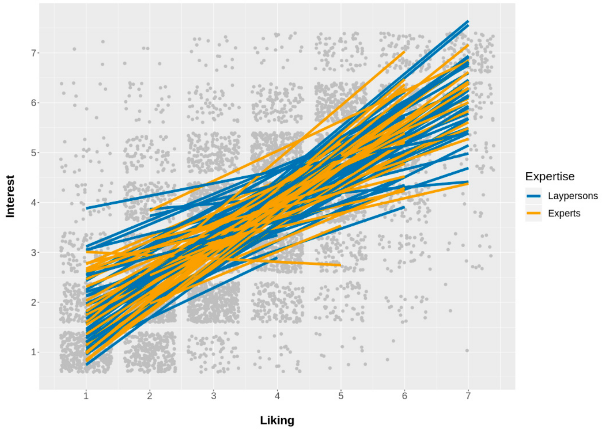
In this part of the experiment, participants were asked to rate all patterns for liking and interest. Liking and interest ratings were strongly correlated. The median Spearman correlation between liking and interest was r_s = 0.68 for both experts and laypersons (difference: 95% HDI [−0.10, 0.10]). See Figure A5 in Appendix A for a “spaghetti” plot of linear regression lines.

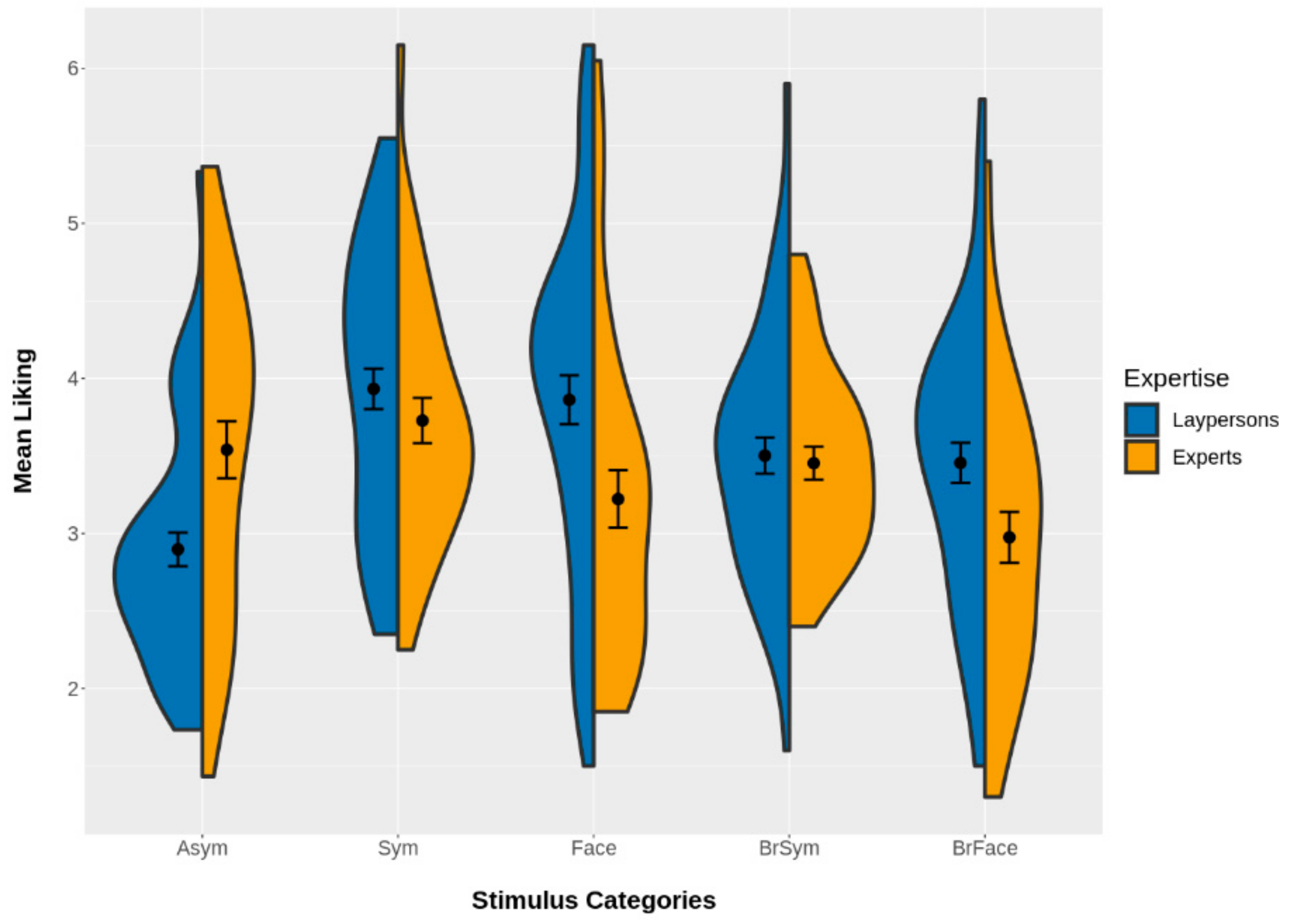
Figure 3 summarizes the means of liking scores for all five stimulus categories (Asym, Sym, Face, BrSym, BrFace) and for experts vs. laypersons. In this figure, one can already see that experts and laypersons differed in their preferences, particularly for the stimulus categories Asym, Face, and BrFace.

In addition, we calculated a Bayesian linear mixed-effects model for liking. Stimulus category and art expertise were dummy coded with base category Asym (vs. Sym, Face, BrSym, and BrFace) and layperson (vs. expert). The applied predictors were as follows: positive and negative affect (PANAS) scores were included to adjust for mood effects. Visual complexity was included to adjust for effects of pattern complexity. Need for cognitive closure (NCC) and its interactions with complexity and with stimulus category were included to adjust for influences of NCC. Finally, expertise and its interactions with complexity and with stimulus category were included, the former to adjust for varying effects of expertise on complexity processing. Of course, the factor of most interest is the interaction of expertise with stimulus category.

Table 2. Population-level (fixed) effects of Bayesian linear mixed-effects model for liking. Decisions about predictors being different from zero are based on the relative positions of the HDIs and the ROPE. Clear decisions are highlighted in boldface. Tendencies are given in parentheses.

Term 1	Estimate	SE	95% HDI	Decision
Intercept	2.96	0.14	[2.69, 3.23]	β > 0
Positive Affect	0.28	0.18	[−0.07, 0.62]	(β ≥ 0)
Negative Affect	−0.16	0.16	[−0.47, 0.16]	?
NCC	0.06	0.19	[−0.32, 0.44]	?
Complexity	0.35	0.10	[0.15, 0.55]	β > 0
Sym vs. Asym	1.01	0.18	[0.65, 1.36]	β > 0
Face vs. Asym	0.98	0.20	[0.59, 1.36]	β > 0
BrSym vs. Asym	0.48	0.16	[0.17, 0.78]	β > 0
BrFace vs. Asym	0.54	0.18	[0.18, 0.89]	β > 0
Expert (vs. Layperson)	0.53	0.21	[0.11, 0.94]	β > 0
NCC × Complexity	−0.08	0.11	[−0.31, 0.14]	?
NCC × Sym vs. Asym	−0.12	0.24	[−0.60, 0.35]	?
NCC × Face vs. Asym	−0.13	0.26	[−0.66, 0.39]	?
NCC × BrSym vs. Asym	−0.01	0.16	[−0.32, 0.31]	?
NCC × BrFace vs. Asym	−0.14	0.22	[−0.57, 0.29]	?
Complexity × Expert	−0.07	0.12	[−0.31, 0.17]	?
Expert × Sym vs. Asym	−0.85	0.25	[−1.33, −0.37]	β < 0
Expert × Face vs. Asym	−1.28	0.27	[−1.81, −0.74]	β < 0
Expert × BrSym vs. Asym	−0.67	0.16	[−1.00, −0.36]	β < 0
Expert × BrFace vs. Asym	−1.13	0.23	[−1.58, −0.68]	β < 0

¹ Note that main effects of predictors involved in interactions are conditional to the interacting variables being zero (i.e., the mean for standardized continuous predictors and the base categories Asym and Laypersons for the categorical predictors).

shows the results of the Bayesian linear mixed-effects model for liking. We found a positive influence of visual complexity (for laypersons) and expertise (for Asym) on liking. Also, the four stimulus categories Sym, Face, BrSym, and BrFace were rated higher for liking than the category Asym by laypersons (because stimulus category is involved in an interaction with expertise, these factors are conditional to the base category of expertise, which is laypersons). Finally, the interactions of expertise with all four factors for the stimulus category were negative. Thus, the effect of higher liking of these categories than the category Asym was reduced for experts.

Because predictors in linear models are conditional to all other factors with which they are involved in interactions, they do not give us all desired comparisons. Therefore, we calculated some selected contrasts (marginal means) from the model which can be found in

Table 3. Selected post-hoc contrasts conditional on stimulus type or participant group for liking. Decisions about contrasts being different from zero are based on the relative positions of the HDIs and the ROPE. Clear decisions are highlighted in boldface. Tendencies are given in parentheses.

Contrast 1	Mean	95% HDI	Decision
Asym: Experts vs. Laypersons	0.53	[0.12, 0.95]	β > 0
Sym: Experts vs. Laypersons	−0.32	[−0.74, 0.14]	?
Face: Experts vs. Laypersons	−0.75	[−1.25, −0.23]	β < 0
BrSym: Experts vs. Laypersons	−0.14	[−0.54, 0.28]	?
BrFace: Experts vs. Laypersons	−0.60	[−1.07, −0.16]	β < 0
Experts: Sym vs. Asym	0.16	[−0.26, 0.57]	?
Experts: Face vs. Asym	−0.30	[−0.76, 0.15]	?
Experts: BrSym vs. Asym	−0.20	[−0.53, 0.13]	?
Experts: BrFace vs. Asym	−0.59	[−1.01, −0.18]	β < 0
Laypersons: Asym vs. Sym	−1.01	[−1.37, −0.66]	β < 0
Laypersons: Face vs. Sym	−0.03	[−0.37, 0.28]	?
Laypersons: BrSym vs. Sym	−0.53	[−0.86, −0.19]	β < 0
Laypersons: BrFace vs. Sym	−0.47	[−0.85, −0.11]	β < 0
Experts: Asym vs. Sym	−0.16	[−0.57, 0.26]	?
Experts: Face vs. Sym	−0.46	[−0.83, −0.08]	β < 0
Experts: BrSym vs. Sym	−0.36	[−0.73, 0.01]	(β ≤ 0)
Experts: BrFace vs. Sym	−0.75	[−1.18, −0.33]	β < 0

¹ Note that these contrasts are also conditional to the NCC predictor being zero (i.e., NCC equal to its global mean, as it is a standardized predictor).

. There, it can be seen that concerning differences between experts and laypersons, experts rated Asym higher than laypersons, but Face and BrFace lower than laypersons. Furthermore, while laypersons rated all four stimulus categories Sym, Face, BrSym, and BrFace higher than Asym (compare Table 2), we only found one difference for experts in BrFace vs. Asym, and this difference is in the opposite direction. In addition, we also calculated contrasts for a different base category: Instead of Asym, this time we chose Sym, as this is the category that generally received the highest liking. Here, we found that while laypersons liked Asym, BrSym, and BrFace less than Sym, experts liked Face and BrFace less than Sym. Furthermore, there was a small tendency that, similar to laypersons, experts did like BrSym less than Sym.

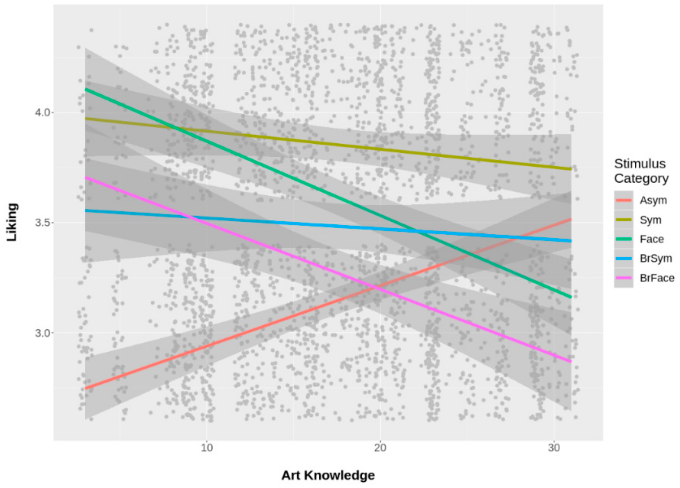
To not solely rely on a dichotomous predictor of art expertise, we also plotted art knowledge vs. liking ratings. Figure A6 in Appendix A shows linear regression lines of art knowledge vs. liking separately for all five categories of stimuli. It can be clearly seen that while liking of category Asym increases, that of Face and BrFace decrease with increasing art knowledge, which is in line with the results of the dichotomous art expertise predictor.

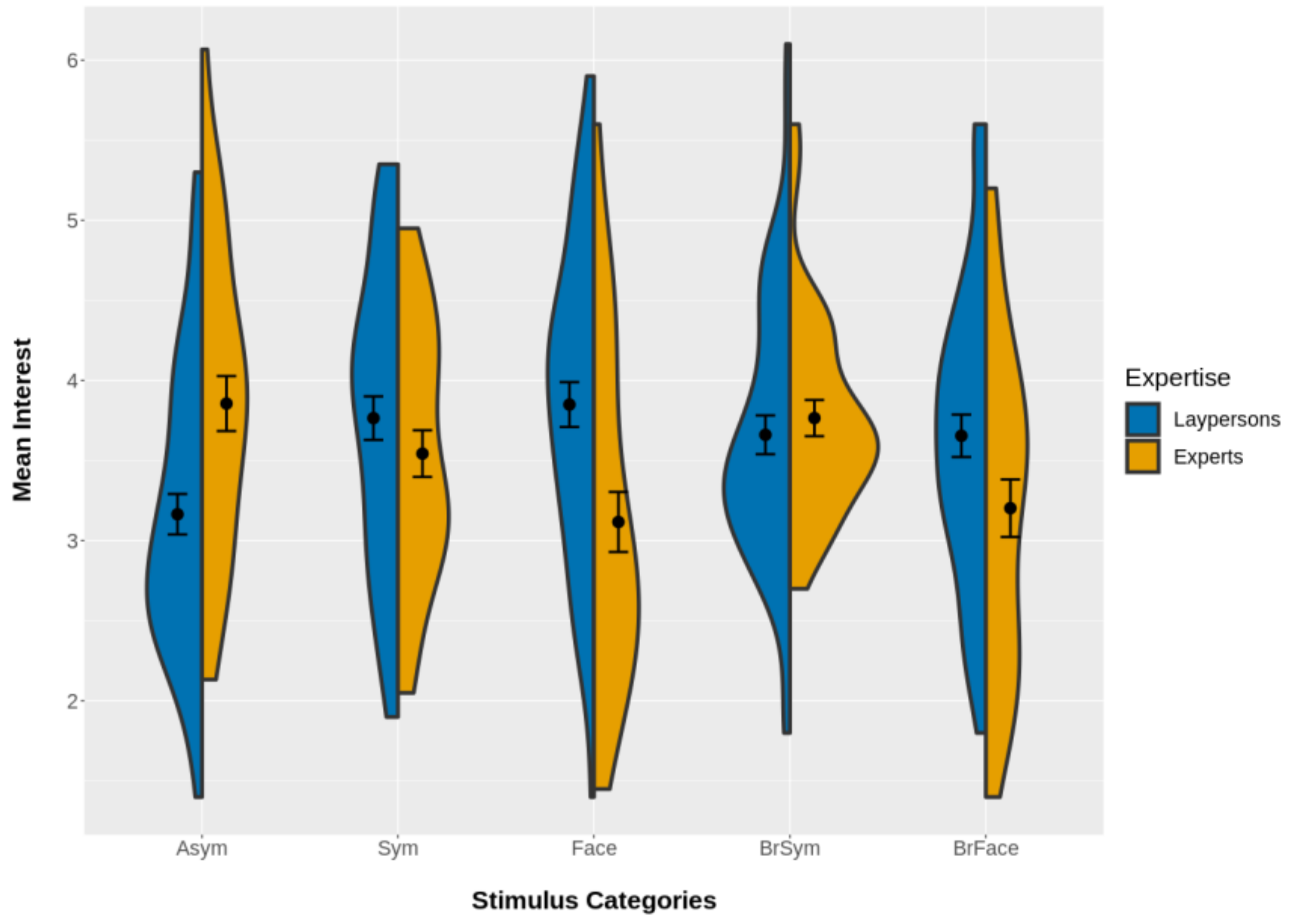
Figure 4 summarizes the means of interest scores for all five stimulus categories and for experts vs. laypersons. The (visual) results seem to be quite similar to liking and the differences between experts and laypersons showed up mostly for the stimulus categories Asym, Face, and BrFace and were in the same directions as liking.

We also calculated a Bayesian linear mixed-effects model for interest with the same predictors as for liking, which is summarized in

Table 4. Population-level (fixed) effects of Bayesian linear mixed-effects model for interest. Decisions about predictors being different from zero are based on the relative positions of the HDIs and the ROPE. Clear decisions are highlighted in boldface. Tendencies are given in parentheses.

Term 1	Estimate	SE	95% HDI	Decision
Intercept	3.25	0.14	[2.98, 3.52]	β > 0
Positive Affect	0.47	0.17	[0.14, 0.81]	β > 0
Negative Affect	−0.04	0.16	[−0.35, 0.28]	?
NCC	−0.16	0.20	[−0.55, 0.23]	?
Complexity	0.47	0.11	[0.25, 0.68]	β > 0
Sym vs. Asym	0.58	0.18	[0.22, 0.94]	β > 0
Face vs. Asym	0.70	0.20	[0.30, 1.10]	β > 0
BrSym vs. Asym	0.40	0.16	[0.09, 0.71]	β > 0
BrFace vs. Asym	0.47	0.20	[0.08, 0.87]	β > 0
Expert (vs. Layperson)	0.48	0.21	[0.07, 0.89]	β > 0
NCC × Complexity	0.00	0.13	[−0.25, 0.25]	?
NCC × Sym vs. Asym	0.18	0.24	[−0.29, 0.64]	?
NCC × Face vs. Asym	0.31	0.28	[−0.24, 0.84]	?
NCC × BrSym vs. Asym	−0.02	0.16	[−0.33, 0.29]	?
NCC × BrFace vs. Asym	0.10	0.24	[−0.38, 0.57]	?
Complexity × Expert	−0.13	0.14	[−0.39, 0.14]	?
Expert × Sym vs. Asym	−0.87	0.25	[−1.36, −0.38]	β < 0
Expert × Face vs. Asym	−1.35	0.29	[−1.91, −0.78]	β < 0
Expert × BrSym vs. Asym	−0.55	0.17	[−0.89, −0.21]	β < 0
Expert × BrFace vs. Asym	−1.09	0.26	[−1.59, −0.58]	β < 0

¹ Note that main effects of predictors involved in interactions are conditional to the interacting variables being zero (i.e., the mean for standardized continuous predictors and the base categories Asym and Laypersons for the categorical predictors).

. Results were very similar to the liking ratings. Basically, the only difference was that in addition, we found a positive influence of positive affect on interest.

We calculated the same additional contrasts as for the model for liking also for interest, which can be found in

Table 5. Selected post-hoc contrasts conditional on stimulus type or participant group for interest. Decisions about contrasts being different from zero are based on the relative positions of the HDIs and the ROPE. Clear decisions are highlighted in boldface. Tendencies are given in parentheses.

Contrast 1	Mean	95% HDI	Decision
Asym: Experts vs. Laypersons	0.48	[0.07, 0.89]	β > 0
Sym: Experts vs. Laypersons	−0.39	[−0.86, 0.05]	?
Face: Experts vs. Laypersons	−0.87	[−1.35, −0.40]	β < 0
BrSym: Experts vs. Laypersons	−0.07	[−0.48, 0.36]	?
BrFace: Experts vs. Laypersons	−0.61	[−1.10, −0.11]	β < 0
Experts: Sym vs. Asym	−0.29	[−0.70, 0.12]	?
Experts: Face vs. Asym	−0.65	[−1.13, −0.18]	β < 0
Experts: BrSym vs. Asym	−0.15	[−0.50, 0.17]	?
Experts: BrFace vs. Asym	−0.62	[−1.05, −0.16]	β < 0
Laypersons: Asym vs. Sym	−0.58	[−0.95, −0.23]	β < 0
Laypersons: Face vs. Sym	0.12	[−0.19, 0.45]	?
Laypersons: BrSym vs. Sym	−0.18	[−0.52, 0.18]	?
Laypersons: BrFace vs. Sym	−0.11	[−0.50, 0.30]	?
Experts: Asym vs. Sym	0.29	[−0.12, 0.70]	?
Experts: Face vs. Sym	−0.36	[−0.73, 0.01]	?
Experts: BrSym vs. Sym	0.14	[−0.23, 0.53]	?
Experts: BrFace vs. Sym	−0.33	[−0.79, 0.11]	?

¹ Note that these contrasts are also conditional to the NCC predictor being zero (i.e., NCC equal to its global mean, as it is a standardized predictor).

. Results are quite similar to liking. The differences in ratings within stimulus categories for experts vs. laypersons are the same for interest as for liking. For the differences between stimulus categories conditional on experts, we found one additional negative effect: experts also found the Face category less interesting than the Asym category. Finally, only one effect was found for the contrasts with Sym as base category (instead of Asym): laypersons found the category Asym less interesting than the category Sym.

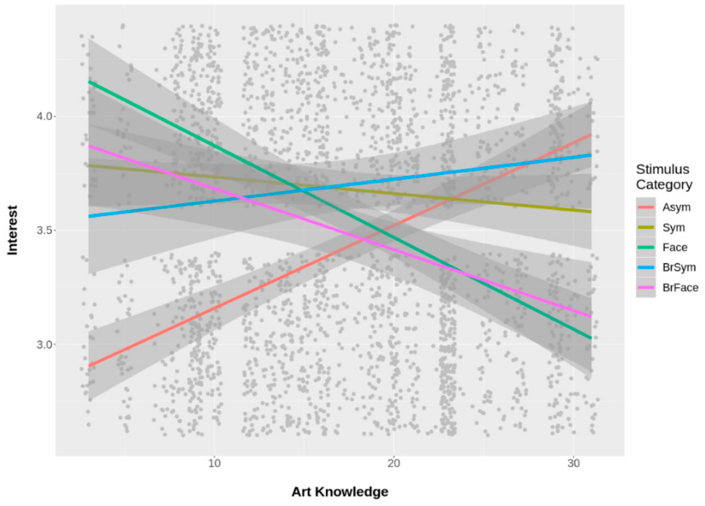
We also plotted art knowledge vs. interest ratings. Figure A7 in Appendix A shows linear regression lines of art knowledge vs. interest separately for all five categories of stimuli. Similar to liking, interest in stimuli of the category Asym increased, while that of Face and BrFace decreased with increasing art knowledge, which was again in line with the results of the dichotomous art expertise predictor.

See Appendix B for additional Bayesian linear mixed-effects models for liking and interest using a continuous predictor of art knowledge instead of the dichotomous predictor of art expertise. Results were rather similar for both predictors.

See Appendix C for additional Bayesian cumulative ordered-probit mixed-effects models for liking and interest. It has been shown that treating ordinal data with metric models can in some cases lead to severe problems [97]. Therefore, we also calculated ordinal models [98]. However, for our data, results were very similar to the traditional metric models presented above.

3.3. Memory Recognition

In this part of the experiment, participants were shown 45 old patterns that they had already seen in the first part and 45 new patterns that they had never seen before. Their task was to indicate whether they had (or had not) already seen the presented patterns.

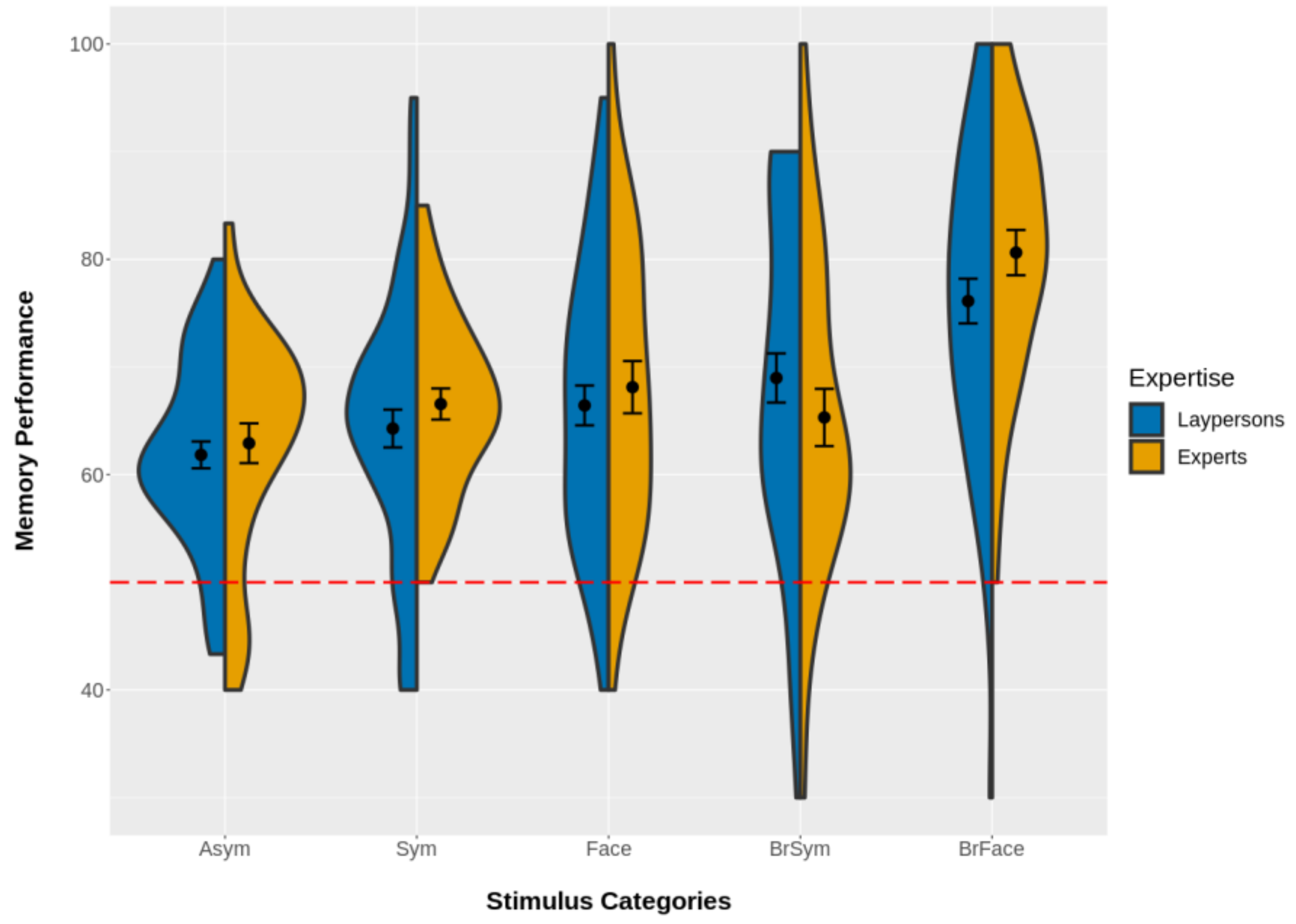
Figure 5 shows the percentages of correct recognition for all five stimulus categories and for experts vs. laypersons. One can already see that this time, there appear to be basically no differences between laypersons and experts, but memory performance seems to differ between stimulus categories. The lowest recognition rates were found for the category Asym; however they were still well above the chance level of 50%.

Here, we calculated a Bayesian logistic mixed-effects model for memory recognition with the same predictors as for liking and for interest which is summarized in

Table 6. Population-level (fixed) effects of Bayesian logistic mixed-effects model for memory recognition. Decisions about predictors being different from zero are based on the relative positions of the HDIs and the ROPE. Clear decisions are highlighted in boldface. Tendencies are given in parentheses.

Term 1	Estimate	SE	95% HDI	Decision
Intercept	0.62	0.19	[0.26, 0.99]	β > 0
Positive Affect	0.03	0.10	[−0.17, 0.23]	?
Negative Affect	0.27	0.10	[0.07, 0.47]	β > 0
NCC	0.09	0.12	[−0.15, 0.34]	?
Complexity	−0.21	0.21	[−0.63, 0.21]	?
Sym vs. Asym	0.04	0.28	[−0.51, 0.59]	?
Face vs. Asym	0.24	0.29	[−0.33, 0.81]	?
BrSym vs. Asym	0.32	0.36	[−0.37, 1.02]	?
BrFace vs. Asym	0.71	0.35	[0.00, 1.41]	(β ≥ 0)
Expert (vs. Layperson)	0.07	0.14	[ −0.19, 0.34]	?
NCC × Complexity	0.11	0.13	[−0.15, 0.37]	?
NCC × Sym vs. Asym	−0.10	0.16	[−0.42, 0.22]	?
NCC × Face vs. Asym	−0.15	0.19	[−0.53, 0.22]	?
NCC × BrSym vs. Asym	−0.02	0.22	[−0.44, 0.40]	?
NCC × BrFace vs. Asym	0.10	0.23	[−0.34, 0.54]	?
Complexity × Expert	0.15	0.14	[−0.13, 0.44]	?
Expert × Sym vs. Asym	0.10	0.17	[−0.24, 0.44]	?
Expert × Face vs. Asym	0.10	0.20	[−0.29, 0.49]	?
Expert × BrSym vs. Asym	−0.23	0.23	[−0.67, 0.22]	?
Expert × BrFace vs. Asym	0.34	0.24	[−0.14, 0.82]	?

¹ Note that main effects of predictors involved in interactions are conditional to the interacting variables being zero (i.e., the mean for standardized continuous predictors and the base categories Asym and Laypersons for the categorical predictors).

. This time, we found only one effect (apart from the intercept): a positive influence of general negative affect on memory recognition.

We also calculated the same additional contrasts for memory recognition as for the models for liking and interest, which can be found in

Table 7. Selected post-hoc contrasts conditional on stimulus type or participant group for memory recognition. Decisions about contrasts being different from zero are based on the relative positions of the HDIs and the ROPE. Clear decisions are highlighted in boldface. Tendencies are given in parentheses.

Contrast1	Mean	95% HDI	Decision
Asym: Experts vs. Laypersons	0.07	[−0.20, 0.33]	?
Sym: Experts vs. Laypersons	0.17	[−0.12, 0.49]	?
Face: Experts vs. Laypersons	0.17	[−0.21, 0.56]	?
BrSym: Experts vs. Laypersons	−0.15	[−0.58, 0.29]	?
BrFace: Experts vs. Laypersons	0.41	[−0.05, 0.87]	(β ≥ 0)
Experts: Sym vs. Asym	0.14	[−0.47, 0.74]	?
Experts: Face vs. Asym	0.34	[−0.28, 0.99]	?
Experts: BrSym vs. Asym	0.10	[−0.65, 0.89]	?
Experts: BrFace vs. Asym	1.05	[0.30, 1.85]	β > 0
Laypersons: Asym vs. Sym	−0.04	[−0.60, 0.50]	?
Laypersons: Face vs. Sym	0.20	[−0.40, 0.80]	?
Laypersons: BrSym vs. Sym	0.28	[−0.45, 1.03]	?
Laypersons: BrFace vs. Sym	0.67	[−0.06, 1.39]	(β ≥ 0)
Experts: Asym vs. Sym	−0.14	[−0.74, 0.47]	?
Experts: Face vs. Sym	0.20	[−0.49, 0.85]	?
Experts: BrSym vs. Sym	−0.04	[−0.87, 0.76]	?
Experts: BrFace vs. Sym	0.91	[0.07, 1.69]	β > 0

¹ Note that these contrasts are also conditional to the NCC predictor being zero (i.e., NCC equal to its global mean, as it is a standardized predictor).

. Similar to laypersons, experts showed higher correct recognition rates for the category BrFace than for the categories Asym and Sym. However, for laypersons, these effects were only tendencies (see Table 6 and Table 7). In addition, there was a small tendency that experts did recognize the category BrFace better than laypersons.

See Appendix B for an additional Bayesian linear mixed-effects model for memory performance using a continuous predictor of art knowledge instead of the dichotomous predictor of art expertise.

4. Discussion

In the present study, we investigated aesthetic evaluation and memory recognition for different abstract (and representational) black-and-white patterns in art experts and laypersons. The motivation for this research is rooted in cognitive theories of empirical aesthetics assuming that aesthetic processing differs between art experts and laypersons [5,6,65]. This is especially the case for the categories abstract vs. representational [62,70,71] but also for symmetric vs. asymmetric [19].

While it was already found that preference for symmetry is less pronounced in art experts than in laypersons [16,18], it was not clear whether the difference in aesthetic evaluation concerning abstract vs. representational art can be similarly found as a preference for abstract over representational patterns in art experts. Specifically, we used five categories of “abstract” patterns (Asym—asymmetric, Sym—symmetric, Face—face-like (symmetric), BrSym—broken symmetric, and BrFace—broken face-like (symmetric); thus, the face-like patterns were no longer abstract in the full sense of the word) as stimuli, presented them to art experts and laypersons which were asked to rate them for liking and interest in the first part, and finally to judge whether they had already seen the patterns before in the second part of the experiment.

Concerning effects of adjustment variables, we found a positive effect of positive affect/mood (PANAS score) on interest ratings (and also a less clear, smaller effect for liking that nevertheless went in the same direction). Thus, participants with a higher positive affect gave higher ratings, which is in line with our assumptions [81]. Also, visual complexity had a positive effect on liking, as well as on interest ratings (both for experts and for laypersons). Because complexity is a secondary factor of aesthetic evaluation with a positive influence on preference for abstract patterns [21,27,103], this is also in line with theory. Finally, we found no effect of need for cognitive closure (NCC). While NCC was negatively correlated with art interest and art knowledge, it had no effect on the ratings. One could assume that a high NCC would be related to higher preference for symmetry and for representational, face-like patterns, as it is also associated with a high desire for order and structure [83]. However, we did not find such an effect, which could of course be due to the effect or our sample simply being rather small.

Our main results can be summarized as follows. While in general symmetric patterns received the highest liking ratings, art experts liked asymmetric abstract patterns more than laypersons. On the other hand, art experts liked representational patterns (pareidolian, face-like patterns) less than laypersons. This was also found for representational patterns that slightly deviated from perfect symmetry (i.e., broken face-like patterns). Furthermore, laypersons liked all other pattern categories (symmetric, face-like, broken symmetric, and broken face-like) better than asymmetric patterns. These factors were included in negative interactions with art expertise, suggesting that these preferences were lower for art experts and only one difference in liking ratings of symmetrical compared with asymmetric patterns was found for art experts; experts liked broken face-like patterns less than asymmetric patterns. Thus, while laypersons liked symmetric patterns better than asymmetric ones, no difference was found for art experts. Results were very similar for interest ratings. Art experts found asymmetric patterns more interesting than laypersons, and face-like and broken face-like patterns less interesting than laypersons. Furthermore, while laypersons found symmetric patterns more interesting than asymmetric ones, no such difference was found for art experts. See the Results section for a more detailed description of differences between art experts and laypersons. Thus, our results are consistent with the findings of Weichselbaum, Leder, and Ansorge [18]. However, for art experts, we found no differences in ratings of asymmetric vs. symmetric patterns and thus no preference for asymmetric over symmetric patterns as in Leder et al. [16].

Furthermore, we did not find differences in memory performance between art experts and laypersons. Concerning differences between stimulus groups, asymmetric patterns generally showed the lowest recognition rates (but still well above chance level), while broken face-like patterns clearly showed the highest recognition rates. Therefore, a memory effect as explanation for the differences in aesthetic evaluations between experts and laypersons is unlikely. For instance, if art experts would have had a better memory for asymmetric patterns, as could have resulted from different encoding of these patterns, this could have been a potential explanation for the higher liking and interest ratings. However, we did not find such a memory effect. The only marginal difference between art experts and laypersons was that experts tended to remember broken face-like patterns slightly better than laypersons. In general, broken face-like patterns were remembered best. One explanation for this memory effect could be that broken face-like patterns might be more distinct than symmetric face-like patterns. It is known that distinctive faces are remembered well (e.g., [104,105]). We also found a positive influence of negative mood on memory performance. This is in line with several studies demonstrating that negative mood can improve memory accuracy [82,106].

One limitation of the current study could be the distinction between art experts and laypersons, as not every student or graduate of art history is necessarily also a high-level art expert and not every student of psychology in necessarily an art layperson. To control for this potentially unclear distinction, we calculated our models both with art expertise as a dichotomous factor (mostly) derived from the study choices of our participants and with art knowledge as a continuous factor based on a questionnaire. The results of both types of models largely agreed. In addition, persons with extremely high art expertise were probably underrepresented in our sample. This is a problem of many studies comparing art experts and laypersons and somewhat limits our conclusions, as we do not know whether the evaluative judgments of high-level experts would have differed from the judgments of our merely mid-level experts. Another limitation is maybe our relatively heterogeneous experimental setup and the two distant sampling timepoints. However, we think that it is unlikely that this has introduced systematic bias into our study and that the use of a Bayesian approach has furthermore helped to avoid some of the pitfalls of classical statistical methods. In addition, while we introduced the stimuli to our participants as abstract patterns—thus, as non-art objects—we cannot fully rule out the possibility that some participants might have also perceived them as artworks. Of course, this would contradict our conclusion that the difference between art experts and laypersons also extends to non-art objects. However, as today everything can potentially be an artwork, it is mostly context and available information that make the difference between an artwork and a non-art object [107,108]. Thus, we think that it is unlikely that our participants have interpreted the presented abstract patterns as artworks.

To sum up, in addition to the effects of art expertise on symmetry preference that are compatible with previous findings [16,18], we also found differences in aesthetic appreciation of representational, face-like patterns between art experts and laypersons. Simply put: While laypersons liked symmetric and face-like (also symmetric) patterns best and asymmetric patterns least, art experts liked symmetric and asymmetric patterns best and face-like patterns least. As also discussed in other studies, we assume that the reason for this striking difference in aesthetic evaluations between art experts and laypersons is rooted in the extensive art-specific training and reflecting on pictures that is necessary to achieve a high level of art expertise [16,58,72,109].

In conclusion, it seems that the well-known fact that, on average, art experts prefer abstract and laypersons representational artworks [66,69,70,71,110] can indeed be extended to “abstract” and “representational” black-and-white patterns, in other words, to non-art objects. Thus, it appears that these differences in aesthetic evaluation between art experts and laypersons are not strictly limited to artworks and likely represent a more general difference in evaluative perceptual judgments.

References

1. Tyler, C.W. Empirical aspects of symmetry perception. Spat. Vis. 1995, 9, 1–7. [Google Scholar] [CrossRef] [PubMed] [Green Version]
2. Wagemans, J. Detection of visual symmetries. Spat. Vis. 1995, 9, 9–32. [Google Scholar] [CrossRef] [PubMed]
3. Wagemans, J. Characteristics and models of human symmetry detection. Trends Cogn. Sci. 1997, 1, 346–352. [Google Scholar] [CrossRef]
4. Arnheim, R. The Power of the Center: A Theory of Composition in the Visual Arts; University of California Press: Los Angeles, CA, USA, 1982. [Google Scholar]
5. Leder, H.; Belke, B.; Oeberst, A.; Augustin, D. A model of aesthetic appreciation and aesthetic judgments. Br. J. Psychol. 2004, 95, 489–508. [Google Scholar] [CrossRef]
6. Leder, H.; Nadal, M. Ten years of a model of aesthetic appreciation and aesthetic judgments: The aesthetic episode—Developments and challenges in empirical aesthetics. Br. J. Psychol. 2014, 105, 443–464. [Google Scholar] [CrossRef]
7. Pecchinenda, A.; Bertamini, M.; Makin, A.D.J.; Ruta, N. The pleasantness of visual symmetry: Always, never or sometimes. PLoS ONE 2014, 9, e92685. [Google Scholar] [CrossRef] [Green Version]
8. Ramachandran, V.; Hirstein, W. The science of art: A neurological theory of aesthetic experience. J. Conscious. Stud. 1999, 6, 15–31. [Google Scholar]
9. Solso, R.L. Cognition and the Visual Arts; MIT Press: Cambridge, MA, USA, 1994. [Google Scholar]
10. Köhler, W. Gestalt Psychology; Liverig: New York, NY, USA, 1929. [Google Scholar]
11. Wagemans, J.; Elder, J.H.; Kubovy, M.; Palmer, S.E.; Peterson, M.A.; Singh, M.; von der Heydt, R. A century of Gestalt psychology in visual perception: I. Perceptual grouping and figure—Ground organization. Psychol. Bull. 2012, 138, 1172–1217. [Google Scholar] [CrossRef] [Green Version]
12. Barlow, H.B.; Reeves, B.C. The versatility and absolute efficiency of detecting mirror symmetry in random dot displays. Vis. Res. 1979, 19, 783–793. [Google Scholar] [CrossRef]
13. Carmody, D.P.; Nodine, C.F.; Locher, P.J. Global detection of symmetry. Percept. Mot. Ski. 1977, 45, 1267–1273. [Google Scholar] [CrossRef]
14. Julesz, B. Foundations of Cyclopean Perception; University of Chicago Press: Chicago, IL, USA, 1971. [Google Scholar]
15. Treder, M.S. Behind the looking-glass: A review on human symmetry perception. Symmetry 2010, 2, 1510–1543. [Google Scholar] [CrossRef]
16. Leder, H.; Tinio, P.P.L.; Brieber, D.; Kröner, T.; Jacobsen, T.; Rosenberg, R. Symmetry is not a universal law of beauty. Empir. Stud. Arts 2019, 37, 104–114. [Google Scholar] [CrossRef] [Green Version]
17. McManus, I. Symmetry and asymmetry in aesthetics and the arts. Eur. Rev. 2005, 13, 157–180. [Google Scholar] [CrossRef]
18. Weichselbaum, H.; Leder, H.; Ansorge, U. Implicit and explicit evaluation of visual symmetry as a function of art expertise. Iperception 2018, 9, 1–24. [Google Scholar] [CrossRef] [PubMed]
19. Lindell, A.K.; Mueller, J. Can science account for taste? Psychological insights into art appreciation. J. Cogn. Psychol. 2011, 23, 453–475. [Google Scholar] [CrossRef]
20. Bertamini, M.; Makin, A. Brain activity in response to visual symmetry. Symmetry 2014, 6, 975–996. [Google Scholar] [CrossRef] [Green Version]
21. Jacobsen, T.; Höfel, L. Aesthetic judgments of novel graphic patterns: Analyses of individual judgments. Percept. Mot. Ski. 2002, 95, 755–766. [Google Scholar] [CrossRef]
22. Jacobsen, T.; Höfel, L. Descriptive and evaluative judgment processes: Behavioral and electrophysiological indices of processing symmetry and aesthetics. Cogn. Affect. Behav. Neurosci. 2003, 3, 289–299. [Google Scholar] [CrossRef]
23. Tinio, P.P.L.; Leder, H. Just how stable are stable aesthetic features? Symmetry, complexity, and the jaws of massive familiarization. Acta Psychol. 2009, 130, 241–250. [Google Scholar] [CrossRef]
24. Bertamini, M.; Makin, A.; Pecchinenda, A. Testing whether and when abstract symmetric patterns produce affective responses. PLoS ONE 2013, 8. [Google Scholar] [CrossRef]
25. Bertamini, M.; Makin, A.; Rampone, G. Implicit association of symmetry with positive valence, high arousal and simplicity. Iperception 2013, 4, 317–327. [Google Scholar] [CrossRef]
26. Friedenberg, J. Geometric regularity, symmetry and the perceived beauty of simple shapes. Empir. Stud. Arts 2018, 36, 71–89. [Google Scholar] [CrossRef] [Green Version]
27. Gartus, A.; Leder, H. The small step toward asymmetry: Aesthetic judgment of broken symmetries. Iperception 2013, 4, 361–364. [Google Scholar] [CrossRef] [PubMed]
28. Gartus, A.; Leder, H. Predicting perceived visual complexity of abstract patterns using computational measures: The influence of mirror symmetry on complexity perception. PLoS ONE 2017, 12, 1–29. [Google Scholar] [CrossRef] [PubMed] [Green Version]
29. Gerger, G.; Leder, H.; Tinio, P.P.L.; Schacht, A. Faces versus patterns: Exploring aesthetic reactions using facial EMG. Psychol. Aesthet. Creat. Arts 2011, 5, 241–250. [Google Scholar] [CrossRef] [Green Version]
30. Höfel, L.; Jacobsen, T. Electrophysiological indices of processing aesthetics: Spontaneous or intentional processes? Int. J. Psychophysiol. 2007, 65, 20–31. [Google Scholar] [CrossRef] [PubMed]
31. Jacobsen, T.; Höfel, L. Aesthetics electrified: An analysis of descriptive symmetry and evaluative aesthetic judgment processes using event-related brain potentials. Empir. Stud. Arts 2001, 19, 177–190. [Google Scholar] [CrossRef]
32. Cárdenas, R.A.; Harris, L.J. Symmetrical decorations enhance the attractiveness of faces and abstract designs. Evol. Hum. Behav. 2006, 27, 1–18. [Google Scholar] [CrossRef]
33. Grammer, K.; Thornhill, R. Human (Homo sapiens) facial attractiveness and sexual selection: The role of symmetry and averageness. J. Comp. Psychol. 1994, 108, 233–242. [Google Scholar] [CrossRef]
34. Little, A.C. Domain specificity in human symmetry preferences: Symmetry is most pleasant when looking at human faces. Symmetry 2014, 6, 222–233. [Google Scholar] [CrossRef] [Green Version]
35. Little, A.C.; Jones, B.C. Attraction independent of detection suggests special mechanisms for symmetry preferences in human face perception. Proc. R. Soc. B Biol. Sci. 2006, 273, 3093–3099. [Google Scholar] [CrossRef] [PubMed] [Green Version]
36. Perrett, D.I.; Burt, D.M.; Penton-Voak, I.S.; Lee, K.J.; Rowland, D.A.; Edwards, R. Symmetry and human facial attractiveness. Evol. Hum. Behav. 1999, 20, 295–307. [Google Scholar] [CrossRef]
37. Perrett, D.I.; Lee, K.J.; Penton-Voak, I. Effects of sexual dimorphism on facial attractiveness. Nature 1998, 394, 884–887. [Google Scholar] [CrossRef] [PubMed]
38. Rhodes, G. The evolutionary psychology of facial beauty. Annu. Rev. Psychol. 2006, 57, 199–226. [Google Scholar] [CrossRef] [PubMed] [Green Version]
39. Rhodes, G.; Proffitt, F.; Grady, J.M.; Sumich, A. Facial symmetry and the perception of beauty. Psychon. Bull. Rev. 1998, 5, 659–669. [Google Scholar] [CrossRef] [Green Version]
40. Bertamini, M.; Rampone, G.; Makin, A.D.J.; Jessop, A. Symmetry preference in shapes, faces, flowers and landscapes. PeerJ 2019, 7, e7078. [Google Scholar] [CrossRef]
41. Makin, A.D.J.; Bertamini, M.; Jones, A.; Holmes, T.; Zanker, J.M. A gaze-driven evolutionary algorithm to study aesthetic evaluation of visual symmetry. Iperception 2016, 7, 1–18. [Google Scholar] [CrossRef] [Green Version]
42. Fink, B.; Neave, N.; Manning, J.T.; Grammer, K. Facial symmetry and judgements of attractiveness, health and personality. Pers. Individ. Dif. 2006, 41, 491–499. [Google Scholar] [CrossRef]
43. Jones, B.C.; Little, A.C.; Penton-Voak, I.S.; Tiddeman, B.P.; Burt, D.M.; Perrett, D.I. Facial symmetry and judgements of apparent health: Support for a “good genes” explanation of the attractiveness-symmetry relationship. Evol. Hum. Behav. 2001, 22, 417–429. [Google Scholar] [CrossRef]
44. Rhodes, G.; Zebrowitz, L.A.; Clark, A.; Kalick, S.M.; Hightower, A.; McKay, R. Do facial averageness and symmetry signal health? Evol. Hum. Behav. 2001, 22, 31–46. [Google Scholar] [CrossRef]
45. Enquist, M.; Arak, A. Symmetry, beauty and evolution. Nature 1994, 372, 169–172. [Google Scholar] [CrossRef] [PubMed]
46. Reber, R.; Schwarz, N.; Winkielman, P. Processing fluency and aesthetic pleasure: Is beauty in the perceiver’s processing experience? Pers. Soc. Psychol. Rev. 2004, 8, 364–382. [Google Scholar] [CrossRef] [PubMed] [Green Version]
47. Reber, R.; Winkielman, P.; Schwarz, N. Effects of perceptual fluency on affective judgments. Psychol. Sci. 1998, 9, 45–48. [Google Scholar] [CrossRef] [Green Version]
48. Reber, R.; Wurtz, P.; Zimmermann, T.D. Exploring “fringe” consciousness: The subjective experience of perceptual fluency and its objective bases. Conscious. Cogn. 2004, 13, 47–60. [Google Scholar] [CrossRef]
49. Shepherd, K.; Bar, M. Preference for symmetry: Only on Mars? Perception 2010, 40, 1254–1256. [Google Scholar] [CrossRef] [Green Version]
50. Mentus, T.; Marković, S. Effects of symmetry and familiarity on the attractiveness of human faces. Psihologija 2016, 49, 301–311. [Google Scholar] [CrossRef] [Green Version]
51. Swaddle, J.; Cuthill, I. Asymmetry and human facial attractiveness: Symmetry may not always be beautiful. Proc. R. Soc. B Biol. Sci. 1995, 261, 111–116. [Google Scholar] [CrossRef]
52. Zaidel, D.W.; Hessamian, M. Asymmetry and symmetry in the beauty of human faces. Symmetry 2010, 2, 136–149. [Google Scholar] [CrossRef] [Green Version]
53. Nadal, M.; Munar, E.; Marty, G.; Cela-Conde, C.J. Visual complexity and beauty appreciation: Explaining the divergence of results. Empir. Stud. Arts 2010, 28, 173–191. [Google Scholar] [CrossRef] [Green Version]
54. Van Geert, E.; Wagemans, J. Order, complexity, and aesthetic appreciation. Psychol. Aesthet. Creat. Arts 2019, 6, 2–10. [Google Scholar] [CrossRef] [Green Version]
55. Berlyne, D.E. Novelty, complexity, and hedonic value. Percept. Psychophys. 1970, 8, 279–286. [Google Scholar] [CrossRef]
56. Berlyne, D.E. Aesthetics and Psychobiology; Appleton Century Crofts: New York, NY, USA, 1971. [Google Scholar]
57. Güçlütürk, Y.; Jacobs, R.H.A.H.; van Lier, R. Liking versus complexity: Decomposing the inverted U-curve. Front. Hum. Neurosci. 2016, 10, 1–11. [Google Scholar] [CrossRef] [PubMed]
58. Silvia, P.J. Artistic training and interest in visual art: Applying the appraisal model of aesthetic emotions. Empir. Stud. Arts 2006, 24, 139–161. [Google Scholar] [CrossRef]
59. Jacobsen, T. Beauty and the brain: Culture, history and individual differences in aesthetic appreciation. J. Anat. 2010, 216, 184–191. [Google Scholar] [CrossRef]
60. Jacobsen, T.; Beudt, S. Stability and variability in aesthetic experience: A review. Front. Psychol. 2017, 8, 1–14. [Google Scholar] [CrossRef] [Green Version]
61. Menninghaus, W.; Wagner, V.; Hanich, J.; Wassiliwizky, E.; Jacobsen, T.; Koelsch, S. The Distancing-Embracing model of the enjoyment of negative emotions in art reception. Behav. Brain Sci. 2017, 40, e347. [Google Scholar] [CrossRef] [Green Version]
62. Cupchik, G.C. From perception to production: A multilevel analysis of the aesthetic process. In Emerging Visions of the Aesthetic Process; Cupchik, G.C., Lászlo, J., Eds.; Cambridge University Press: New York, NY, USA, 1992; pp. 83–99. [Google Scholar]
63. Kirk, U.; Skov, M.; Christensen, M.S.; Nygaard, N. Brain correlates of aesthetic expertise: A parametric fMRI study. Brain Cogn. 2009, 69, 306–315. [Google Scholar] [CrossRef]
64. Augustin, D.; Leder, H. Art expertise: A study of concepts and conceptual spaces. Psychol. Sci. 2006, 48, 135–156. [Google Scholar]
65. Van Paasschen, J.; Bacci, F.; Melcher, D.P. The influence of art expertise and training on emotion and preference ratings for representational and abstract artworks. PLoS ONE 2015, 10, e0134241. [Google Scholar] [CrossRef] [Green Version]
66. Leder, H.; Gerger, G.; Dressler, S.G.; Schabmann, A. How art is appreciated. Psychol. Aesthet. Creat. Arts 2012, 6, 2–10. [Google Scholar] [CrossRef]
67. Leder, H.; Gerger, G.; Brieber, D.; Schwarz, N. What makes an art expert? Emotion and evaluation in art appreciation. Cogn. Emot. 2014, 28, 1137–1147. [Google Scholar] [CrossRef] [PubMed]
68. Silvia, P.J. Interested experts, confused novices: Art expertise and the knowledge emotions. Empir. Stud. Arts 2013, 31, 107–115. [Google Scholar] [CrossRef]
69. Hekkert, P.; Van Wieringen, P.C.W. The impact of level of expertise on the evaluation of original and altered versions of post-impressionistic paintings. Acta Psychol. 1996, 94, 117–131. [Google Scholar] [CrossRef]
70. Pihko, E.; Virtanen, A.; Saarinen, V.-M.; Pannasch, S.; Hirvenkari, L.; Tossavainen, T.; Haapala, A.; Hari, R. Experiencing art: The influence of expertise and painting abstraction level. Front. Hum. Neurosci. 2011, 5, 94. [Google Scholar] [CrossRef] [PubMed] [Green Version]
71. Bimler, D.L.; Snellock, M.; Paramei, G.V. Art expertise in construing meaning of representational and abstract artworks. Acta Psychol. 2019, 192, 11–22. [Google Scholar] [CrossRef] [PubMed]
72. Verpooten, J.; Dewitte, S. The conundrum of modern art: Prestige-driven coevolutionary aesthetics trumps evolutionary aesthetics among art experts. Hum. Nat. 2017, 28, 16–38. [Google Scholar] [CrossRef]
73. Steiner, W. Venus in Exile: The Rejection of Beauty in 20th-Century Art; Free Press: New York, NY, USA, 2001. [Google Scholar]
74. Bar, M. Visual objects in context. Nat. Rev. Neurosci. 2004, 5, 617–629. [Google Scholar] [CrossRef]
75. Oliva, A.; Torralba, A. Building the gist of a scene: The role of global image features in recognition. Prog. Brain Res. 2006, 155, 23–36. [Google Scholar] [CrossRef]
76. Krohne, H.W.; Egloff, B.; Kohlmann, C.-W.; Tausch, A. Untersuchungen mit einer deutschen Version der “positive and negative affect schedule” (PANAS). Diagnostica 1996, 42, 139–156. [Google Scholar]
77. Schlink, S.; Walther, E. Kurz und gut: Eine deutsche Kurzskala zur Erfassung des Bedürfnisses nach kognitiver Geschlossenheit. Zeitschrift Für Sozialpsychologie 2007, 38, 153–161. [Google Scholar] [CrossRef]
78. Specker, E.; Forster, M.; Brinkmann, H.; Boddy, J.; Pelowski, M.; Rosenberg, R.; Leder, H. The Vienna art interest and art knowledge questionnaire (VAIAK): A unified and validated measure of art interest and art knowledge. Psychol. Aesthet. Creat. Arts 2018. [Google Scholar] [CrossRef]
79. Mathôt, S.; Schreij, D.; Theeuwes, J. Open Sesame: An open-source, graphical experiment builder for the social sciences. Behav. Res. Methods 2012, 44, 314–324. [Google Scholar] [CrossRef] [PubMed] [Green Version]
80. Watson, D.; Clark, L.A.; Tellegen, A. Development and validation of brief measures of positive and negative affect: The PANAS scales. J. Pers. Soc. Psychol. 1988, 54, 1063–1070. [Google Scholar] [CrossRef] [PubMed]
81. Forgas, J.P. Mood and judgment: The affect infusion model (AIM). Psychol. Bull. 1995, 117, 39–66. [Google Scholar] [CrossRef]
82. Forgas, J.P. Don’t worry, be sad! On the cognitive, motivational, and interpersonal benefits of negative mood. Curr. Dir. Psychol. Sci. 2013, 22, 225–232. [Google Scholar] [CrossRef] [Green Version]
83. Webster, D.M.; Kruglanski, A.W. Individual differences in need for cognitive closure. J. Pers. Soc. Psychol. 1994, 67, 1049–1062. [Google Scholar] [CrossRef]
84. Judd, C.M.; Westfall, J.; Kenny, D.A. Treating stimuli as a random factor in social psychology: A new and comprehensive solution to a pervasive but largely ignored problem. J. Pers. Soc. Psychol. 2012, 103, 54–69. [Google Scholar] [CrossRef] [Green Version]
85. Gelman, A. The failure of null hypothesis significance testing when studying incremental changes, and what to do about it. Pers. Soc. Psychol. Bull. 2017, 44, 16–23. [Google Scholar] [CrossRef]
86. McShane, B.B.; Gal, D.; Gelman, A.; Robert, C.; Tackett, J.L. Abandon statistical significance. Am. Stat. 2019, 73, 235–245. [Google Scholar] [CrossRef] [Green Version]
87. Wagenmakers, E.-J. A practical solution to the pervasive problems of p values. Psychon. Bull. Rev. 2007, 14, 779–804. [Google Scholar] [CrossRef] [Green Version]
88. Kruschke, J.K.; Liddell, T.M. Bayesian data analysis for newcomers. Psychon. Bull. Rev. 2018, 25, 155–177. [Google Scholar] [CrossRef] [PubMed] [Green Version]
89. Van der Linden, S.; Chryst, B. No need for Bayes factors: A fully Bayesian evidence synthesis. Front. Appl. Math. Stat. 2017, 3, 472–482. [Google Scholar] [CrossRef] [Green Version]
90. R Core Team. R: A Language and Environment for Statistical Computing; R Foundation for Statistical Computing: Vienna, Austria, 2019; Available online: https://www.r-project.org (accessed on 2 May 2020).
91. Wickham, H. Tidyverse: Easily Install and Load the “Tidyverse”; R Package Version; R Core Team: Vienna, Austria, 2019; Available online: https://github.com/tidyverse/tidyverse (accessed on 2 May 2020).
92. Bürkner, P.-C. brms: An R package for Bayesian multilevel models using Stan. J. Stat. Softw. 2017, 80, 1–28. [Google Scholar] [CrossRef] [Green Version]
93. Bürkner, P.-C. Advanced Bayesian multilevel modeling with the R package brms. R J. 2018, 10, 395. [Google Scholar] [CrossRef]
94. Carpenter, B.; Gelman, A.; Hoffman, M.D.; Lee, D.; Goodrich, B.; Betancourt, M.; Brubaker, M.; Guo, J.; Li, P.; Riddell, A. Stan: A probabilistic programming language. J. Stat. Softw. 2017, 76. [Google Scholar] [CrossRef] [Green Version]
95. Gelman, A.; Rubin, D.B. Inference from iterative simulation using multiple sequences. Stat. Sci. 1992, 7, 457–472. [Google Scholar] [CrossRef]
96. Gelman, A. Scaling regression inputs by dividing by two standard deviations. Stat. Med. 2008, 27, 2865–2873. [Google Scholar] [CrossRef]
97. Liddell, T.M.; Kruschke, J.K. Analyzing ordinal data with metric models: What could possibly go wrong? J. Exp. Soc. Psychol. 2018, 79, 328–348. [Google Scholar] [CrossRef] [Green Version]
98. Bürkner, P.-C.; Vuorre, M. Ordinal regression models in psychology: A tutorial. Adv. Methods Pract. Psychol. Sci. 2019, 2, 77–101. [Google Scholar] [CrossRef] [Green Version]
99. Lenth, R.; Singmann, H.; Love, J.; Buerkner, P.; Herve, H. Emmeans: Estimated Marginal Means, Aka Least-Squares Means; R Package Version; R Core Team: Vienna, Austria, 2019; Available online: https://github.com/rvlenth/emmeans (accessed on 2 May 2020).
100. Kay, M. Tidybayes: Tidy Data and Geoms for Bayesian Models; R Package Version; R Core Team: Vienna, Austria, 2019; Available online: http://mjskay.github.io/tidybayes (accessed on 2 May 2020).
101. Wickham, H. Ggplot2: Elegant Graphics for Data Analysis; Springer: New York, NY, USA, 2016; Available online: https://ggplot2.tidyverse.org (accessed on 2 May 2020).
102. Bååth, R. Bayesian First Aid: A package that implements bayesian alternatives to the classical *. test functions in R. In Proceedings of the UseR! 2014—The International R User Conference, Los Angeles, CA, USA, 30 June–3 July 2014. [Google Scholar]
103. Eisenman, R.; Gellens, H. Preferences for complexity-simplicity and symmetry-asymmetry. Percept. Mot. Ski. 1968, 26, 888–890. [Google Scholar] [CrossRef]
104. Leder, H.; Bruce, V. Local and relational aspects of face distinctiveness. Q. J. Exp. Psychol. A 1998, 51, 449–473. [Google Scholar] [CrossRef] [PubMed]
105. Valentine, T. A unified account of the effects of distinctiveness, inversion, and race in face recognition. Q. J. Exp. Psychol. Sect. A 1991, 43, 161–204. [Google Scholar] [CrossRef] [PubMed]
106. Forgas, J.P.; Goldenberg, L.; Unkelbach, C. Can bad weather improve your memory? An unobtrusive field study of natural mood effects on real-life memory. J. Exp. Soc. Psychol. 2009, 45, 254–257. [Google Scholar] [CrossRef]
107. Gerger, G.; Leder, H.; Kremer, A. Context effects on emotional and aesthetic evaluations of artworks and IAPS pictures. Acta Psychol. 2014, 151, 174–183. [Google Scholar] [CrossRef]
108. Kirk, U.; Skov, M.; Hulme, O.; Christensen, M.S.; Zeki, S. Modulation of aesthetic value by semantic context: An fMRI study. Neuroimage 2009, 44, 1125–1132. [Google Scholar] [CrossRef]
109. Belke, B.; Leder, H.; Harsanyi, G.; Carbon, C.C. When a Picasso is a “Picasso”: The entry point in the identification of visual art. Acta Psychol. 2010, 133, 191–202. [Google Scholar] [CrossRef]
110. Marković, S. Perceptual, semantic and affective dimensions of experience of abstract and representational paintings. Psihologija 2011, 44, 191–210. [Google Scholar] [CrossRef]
Figure 1. Examples of stimulus patterns from all five stimulus categories (and nine groups) used in the main study: asymmetric (Asym), symmetric (Sym), symmetric face-like (Face), broken symmetric (BrSym), and broken symmetric face-like (BrFace) patterns. The blue area comprises the five categories and the grey area shows examples of additional patterns included to match the increased visual complexity of the broken patterns (compare Table 1).
Symmetry 12 00707 g001
Figure 2. Box and violin plots of art knowledge scores for the three groups of laypersons, art history students, and art history graduates. The box plots depict the median as a bold horizontal line and the interquartile range as a box, as well as extremes and outliers, while the violin plots show a kernel density estimate of the full distribution. Note that three students of art history had very low scores of art knowledge and were removed from the sample, while three laypersons had very high scores and were therefore considered to be art experts.
Symmetry 12 00707 g002
Figure 3. Split violin plots showing a kernel density estimate of the full distributions of mean liking ratings for stimulus categories and for experts vs. laypersons. The black dots depict the mean and error bars depict standard error of the mean.
Symmetry 12 00707 g003
Figure 4. Split violin plots showing a kernel density estimate of the full distributions of mean interest ratings for stimulus categories and for experts vs. laypersons. The black dots depict the mean and error bars depict standard error of the mean.
Symmetry 12 00707 g004
Figure 5. Split violin plots showing a kernel density estimate of the full distributions of mean percentage of memory performance (correct recognition) for stimulus categories and for experts vs. laypersons. The black dots depict the mean and error bars depict standard error of the mean. The dotted red line corresponds to chance level performance of 50%.
Symmetry 12 00707 g005