Abstract
In scientific disciplines and other engineering applications, most of the systems refer to uncertainties, because when modeling physical systems the uncertain parameters are unavoidable. In view of this, it is important to investigate dynamical systems with uncertain parameters. In the present study, a delay-dividing approach is devised to study the robust stability issue of uncertain neural networks. Specifically, the uncertain stochastic complex-valued Hopfield neural network (USCVHNN) with time delay is investigated. Here, the uncertainties of the system parameters are norm-bounded. Based on the Lyapunov mathematical approach and homeomorphism principle, the sufficient conditions for the global asymptotic stability of USCVHNN are derived. To perform this derivation, we divide a complex-valued neural network (CVNN) into two parts, namely real and imaginary, using the delay-dividing approach. All the criteria are expressed by exploiting the linear matrix inequalities (LMIs). Based on two examples, we obtain good theoretical results that ascertain the usefulness of the proposed delay-dividing approach for the USCVHNN model.
1. Introduction
Over the past two decades, the dynamic analysis for different types of neural networks (NNs), including cellular NNs, recurrent NNs, static NNs, generalized NNs, bi-directional associative memory NNs, memristor NNs, Cohen-Grossberg NNs, fractional-order NNs, have received remarkable attention due to their successful applications [1,2,3,4,5,6,7,8]. In this domain, the Hopfield Neural Network (HNN) has been considered as an attractive model due to its robust mathematical capability [9]. Indeed, HNN-related models have received significant research attention in both areas of mathematical and practical analysis [10,11,12,13].
Time delays naturally occur in practical systems. They are normally viewed as the main source of chaos, leading to a poor performance as well as causing system instability. As a result, the study of NNs with time-delays is important [11,12,13,14]. On the other hand, as mentioned in References [15,16,17], stochastic inputs affect the stability of NNs. As such, the stochastic effects must be taken into consideration in stability analysis of NNs. Accordingly, several stability methods for HNNs with stochastic effects have been published recently [10,11,12,13,18,19,20,21,22]. As an example, Wan and Sun in Reference [19] discussed the mean square exponential stability pertaining to a NN, as in (1)
Later, in Reference [20], the authors generalized the model proposed in Reference [19]. The exponential stability of NNs has also been analysed, as in (2)
where is the state vector; is the Brownian motion. Note that denotes the self-feedback weight, while and denote the interconnection matrices that contain the neuron weight coefficients. In addition, denotes to the transmission delay; denotes the corresponding output of the jth unit; and denotes the density of stochastic effects.
On the other hand, CVNN has been commonly used in various areas, such as image processing, computer vision, electromagnetic waves, speech synthesis, sonic waves, quantum devices and so in References [23,24,25]. Recently, due to good applicability, CVNNs have attracted tremendous interest from the research community [26,27,28,29,30,31,32,33,34,35,36,37,38,39,40,41]. In general, a CVNN model comprises complex-valued variables as compared with those of real-valued NNs. These complex-valued variables include the inputs, states, connection weights, as well as activation functions. Therefore, a lot of investigations on CVNNs have been conducted. Recent studies mainly focus on their complex behaviors, including global asymptotic stability [26,27,28,29,30,31,32,33,34,35,36,37,38,39,40,41,42], global exponential stability [28,29], state estimation of CVNNs [30,31]. As an example, in Reference [13], several sufficient conditions are derived by separating the real and imaginary parts in a CVNN. The results confirm that the global asymptotic stability pertaining to the considered CVNN. Similarly, some other stability conditions have been defined for CVNNs [32,33,34,35,36,37,38,39,40,41]. However, it should be noted that the robust stability issue with respect to uncertain stochastic complex-valued Hopfield neural networks (USCVHNNs) with time delays is yet to be fully investigated. This forms the motivation of the present research.
This article focuses on the robust stability issue of the USCVHNN model. Firstly, we formulate a general form of the system model by considering both aspects of parameter uncertainties and stochastic effects. Based on the studies in References [42,43], we divide the delay interval into N equivalent sub-intervals. Then, we exploit the homeomorphism principle along with the Lyapunov function and other analytical methods in our analysis. Specifically, we derive new sufficient conditions with respect to the robust stability issue of a USCVHNN model in terms of linear matrix inequalities (LMIs). We obtain the feasible solutions by using the MATLAB software package. Finally, the obtained theoretical results are validated by two examples. The remaining part of this paper is organized as follows. In Section 2, we formally define the proposed model. In Section 3, we explain the new stability criterion. In Section 4, we present the numerical examples and the associated simulation results. Concluding remarks are given in Section 5.
Notations: in this article, the Euclidean n-space and real matrices are denoted by and , respectively. Note that i represents the imaginary unit, that is, . In addition, and denote the n dimensional complex vectors and complex matrices, respectively. The complex conjugate transpose and matrix transposition are denoted by the superscripts * and T, respectively. Besides that, a matrix indicates that is a positive (negative) definite matrix. On the other hand, denotes the diagonal of the block diagonal matrix, while denotes an identity matrix, while ☆ indicates a symmetric term in a matrix. Finally, stands for mathematical expectation, , and indicates a complete probability space with a filtration .
2. Problem Statement and Mathematical Preliminaries
Motivated by Wang et al. [13], we consider the following CVHNN model with a time-varying delay:
where denotes state vector; and indicate the self-feedback connection weights as well as the interconnection matrix representing neuron weight coefficients, respectively. In addition, is the neuron activation function; indicates the external input vector, while is the initial condition. Note that is the time-varying delay, which satisfies the following conditions
where and are real known constants.
To derive new stability criterion for the CVNN model in (5), we use the delay-dividing method by dividing into several intervals using an integer N with the length of each interval denoted by ; as follows
where denotes a portion of the time-varying delay , which satisfies
where and .
Assumption 1.
The activation function , is able to satisfy the Lipschitz condition for all , that is,
where is a constant.
From Assumption 1, one can obtain
where .
Remark 1.
Assumption 1 is a generalization of the real-valued function that is able to satisfy the Lipschitz condition on . In addition, it is valid by dividing its real and imaginary parts.
It must be noticed that, in a realistic analysis, the uncertainties associated with the neuron weight coefficients are unavoidable. Besides that, the network model is susceptible to the stochastic effects. As a result, it is important to take the parameter uncertainties and stochastic disturbances into account when analysing the stability of NN models. Therefore, the model in (5) can be stated as
where are the known constant matrices, and is the n dimensional Brownian motion defined on .
It is assumed that the parameter uncertainties in (10) are able to satisfy:
where and are the known real matrices, while is the time-varying uncertain matrix that satisfies
We define , where i shows the imaginary unit.
Now, the CVNN model in (10) can be separated into both the real and imaginary parts, that is,
Let
Then, the model in (15) can be equivalently re-written as
From (9) one can obtain
where .
The model in (16) has the following initial condition:
where .
Remark 2.
It should be noted that, if we let and , where ν is a constant, the model in (16) turns out to be the subsequent CVNN of
Lemma 1.
[41] Let be a continuous map. It satisfies the following conditions:
- (i)
- is injective on
- (ii)
- as , then is a homeomorphism on .
Lemma 2.
[41] Given any vectors of the form , along with a positive-definite matrix as well as a scalar , the following inequality is always true:
Lemma 3.
[44] Let and be real matrices, satisfies . In this respect, , iff there exist a scalar such that or equivalently
3. An Analysis of Uniqueness and Stability
In this sub-section, we present the sufficient conditions for the existence, uniqueness, as well as global asymptotic stability of the considered CVNN model.
3.1. Delay-Independent Stability Criteria
Theorem 1.
Based on Assumption 1, we can divide the activation function into two parts: real and imaginary. The model in (20) has a unique equilibrium point. The model is deemed globally asymptotically stable if there exist matrix and scalar that are able to satisfy the following LMI:
Proof.
A map associated with (20) is defined, that is,
We prove that the map is injective by contradiction. Given and with such that , it follows that
Multiplying both sides of (23) by yields
Taking the transpose on (24), we have
From Lemma (2) and (26), we have
Since is a positive constant, we can obtain from (18) that
If (21) holds, by Schur complement, we have
In addition we prove that as . Based on (30) we have
for sufficiently small . By using the same derivation method of (29), we have
One can obtain from (32) that
As a result, we have as .
We can see from Lemma 1 that the map is homeomorphic on . In addition, there exists a unique point such that . Therefore, the model in (20) has a unique equilibrium point .
Now, we prove the global asymptotic stability of the equilibrium point possessed by the model in (20). Based on the transformation , the equilibrium point of the model in (20) can be converted to the origin. As such, we have
where .
To analyse the global asymptotic stability with respect to the equilibrium point of the model in (34), the Lyapunov functional is utilized, that is,
where and . As a result, the time derivative of and the solution of the model in (35) yields
It is easy to observe that if and only if and
3.2. Delay-Dependent Stability Criteria
In this section, we address the delay-dependent stability criteria for the model in (16) using the delay-dividing method.
Theorem 2.
Based on Assumption 1, we can divide the activation function into two parts: real and imaginary. For given scalars and , the model in (16) is robust as well as globally asymptotically stable in the mean square, subject to the existence of matrices and positive scalars in a way that the following LMI is satisfied:
where
Proof.
The Lyapunov function candidate pertaining to the model in (16) is formed as follows:
Based on the It’s differential rule, we can obtain the stochastic derivative of along with the trajectories of the model in (16) as follows:
Based on Lemma (3),
By using Schur complement lemma, can be written as .
As a result,
It can be easily deduced that for , there must exist a scalar such that
By taking the mathematical expectation on both sides of the model in (47),
The above result indicates that the model in (16) is robust. it is also globally asymptotically stable in the mean square. This completes the proof. □
Remark 3.
The delay-dividing number N is a positive integer and, at the same time, N should not be lower than 2. This conservatism is reduced as N increases, and the time-delay tends to approach certain upper boundary. When N equals to 2 or 3, the conservatism is small enough.
Remark 4.
In the situation where no uncertainties exist, the model in (10) becomes
Simultaneously, the model in (16) becomes
Corollary 1 is obtained by setting in the proof of Theorem (2).
Corollary 1.
Based on Assumption 1, we can divide the activation function into two parts: real and imaginary. For given scalars and , the model in (51) is globally asymptotically stable in the mean square, subject to the existence of matrices and positive scalars in a way that the following LMI is satisfied:
where
Remark 5.
In the situation where no uncertainties and stochastic effects exist, the model in (10) becomes
Simultaneously, the model in (16) becomes
Corollary 2 is obtained by setting in the proof of Theorem 2.
Corollary 2.
Based on Assumption 1, we can divide the activation function into two parts: real and imaginary. For given scalars and , the model in (54) is globally asymptotically stable, subject to the existence of matrices and positive scalars is a way that the following LMI is satisfied:
where
Remark 6.
It should be noticed that, due to the existence of modeling errors and measurement errors, we cannot solve some of the problems by using an exact mathematical model in realistic scenarios. The model described in this paper contains the following parameter uncertainties . As a result, it is assumed that the effects of parameter uncertainties in our study are under the time-varying and norm-bounded condition.
Remark 7.
It is worth noting that several stability results have been published recently without taking into account the parameter uncertainties and stochastic effects on CVNNs [26,27]. In this paper, we take into account both the parameter uncertainties and stochastic effects. Therefore, this paper includes more general stability criteria than those in References [26,27].
4. Illustrative Examples
Here, two numerical examples are provided to ascertain the usefulness of the derived outcomes presented in the previous section.
Example 1.
The CVNN model defined in (10) that contains the following parameters is considered:
Assume that . We can obtain the following based on a simple calculation:
When , which satisfies and . By using the MATLAB software package, the LMI condition of (40) in Theorem (2) is true.
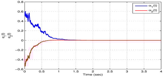
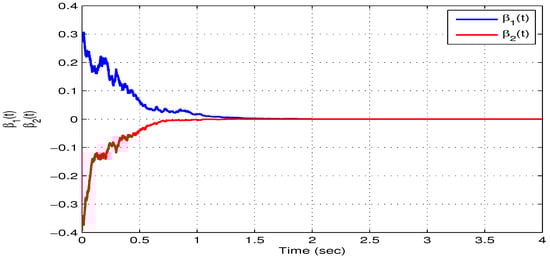
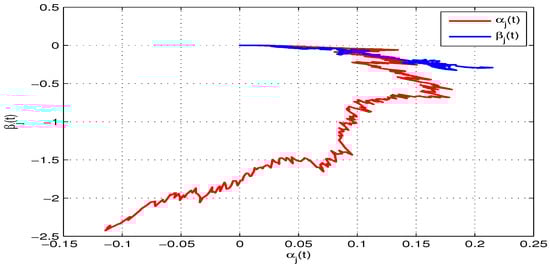
Based on the initial values and , Figure 1 and Figure 2 depict the state trajectories pertaining to both the real and imaginary parts of the model in (10). On the other hand, Figure 3 illustrates the phase trajectories pertaining to both the real and imaginary parts of the model in (10). It is obvious form Figure 1, Figure 2 and Figure 3 that the model converges to an equilibrium point, which means that the model in (10) or equivalently the model in (16) is robust as well as globally asymptotically stable.
Figure 1.
An illustration of the state trajectories of the real part for the model in (10) with respect to Example 1.
Figure 2.
An illustration of the state trajectories of the imaginary part for the model in (10) with respect to Example 1.
Figure 3.
An illustration of the phase trajectories between the real and imaginary subspace of the model in (10).
Example 2.
The CVNN model defined in (53) that contains the following parameters is considered:
By assuming that , we can obtain the following by simple calculation
When , which satisfying and . By using the MATLAB software package, it is found that the LMI of (55) is feasible. Table 1 shows the maximum allowable upper bound of under various settings. Figure 4 and Figure 5 depict the state trajectories with respect to the real and imaginary parts of the model in (53), in which 20 initial values that are randomly selected within a bounded interval are considered. On the other hand, Figure 6 and Figure 7 depict the phase trajectories with respect to the real and imaginary parts of the model in (53). From Corollary 2, we can confirm that the equilibrium point of the model in (53) or equivalently the model in (54), is globally asymptotically stable.

Table 1.
The maximum allowable upper bounds of for different settings in Example 2.
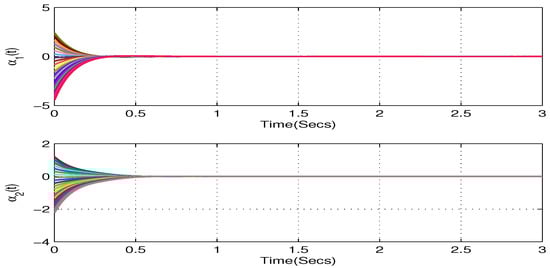
Figure 4.
An illustration of the state trajectories of the real part for the model in (53) with respect to Example 2.
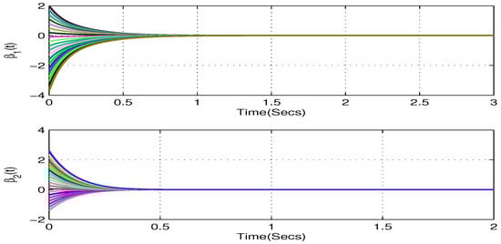
Figure 5.
An illustration of the state trajectories of the imaginary part for the model in (53) with respect to Example 2.
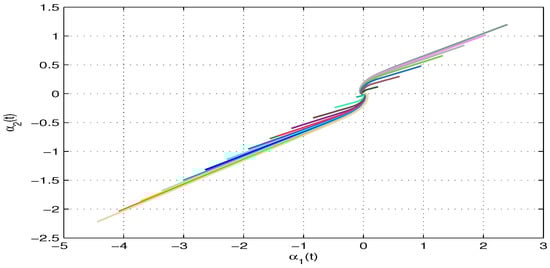
Figure 6.
An illustration of the phase trajectories between the real subspace for the model in (53).
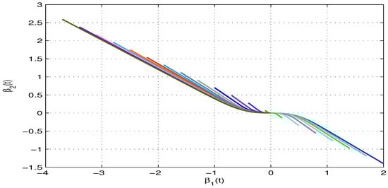
Figure 7.
An illustration of the phase trajectories between the real subspace for the model in (53).
5. Conclusions
In this paper, we have investigated the robust stability issue of the USCVHNN models along with the consideration with their time-varying delay and stochastic effects. Based on the delay-dividing approach, we have formulated a more general form of the model under scrutiny by incorporating the parameter uncertainties and stochastic effects. Following the studies in References [42,43], we have divided the delay interval into N equivalent sub-intervals. In addition, we have exploited the homeomorphism principle along with the Lyapunov function and other analytical methods in our analysis. As a results, we have derived new sufficient conditions in terms of LMIs, which allow us to analyse the robust stability issues pertaining to USCVHNN models. The feasible solutions have been obtained by using the MATLAB software package. Finally, the obtained theoretical results are ascertained through two numerical examples.
For further research, we will extend our proposed approach to analysing other relevant types of CVNN models. In this regard, we intend to undertake an investigation of the fuzzy stochastic CVNN models.
Author Contributions
Funding acquisition, P.C.; Conceptualization, G.R.; Software, P.C., P.K., U.H., R.R. and R.S.; Formal analysis, G.R.; Methodology, G.R.; Supervision, C.P.L.; Writing—original draft, G.R.; Validation, G.R.; Writing—review and editing, G.R. All authors have read and agreed to the published version of the manuscript.
Funding
This research is made possible through financial support of Chiang Mai University.
Acknowledgments
The authors are grateful to the support provided by Chiang Mai University.
Conflicts of Interest
The authors declare no conflict of interest.
References
- Arik, S. An analysis of global asymptotic stability of delayed cellular neural networks. IEEE Trans. Neural Netw. 2002, 13, 1239–1242. [Google Scholar] [CrossRef]
- Liang, S.; Cao, J. A based-on LMI stability criterion for delayed recurrent neural networks. Chaos Soliton. Fract. 2006, 28, 154–160. [Google Scholar] [CrossRef]
- Cao, J. Global asymptotic stability of neural networks with transmission delays. Int. J. Syst. Sci. 2000, 31, 1313–1316. [Google Scholar] [CrossRef]
- Wu, Z.G.; Lam, J.; Su, H.; Chu, J. Stability and dissipativity analysis of static neural networks with time delay. IEEE Trans. Neural Netw. Learn. Syst. 2012, 23, 199–210. [Google Scholar] [PubMed]
- Chen, G.; Xia, J.; Zhuang, G. Delay-dependent stability and dissipativity analysis of generalized neural networks with Markovian jump parameters and two delay components. J. Frankl. Inst. 2016, 353, 2137–2158. [Google Scholar] [CrossRef]
- Zhu, Q.; Cao, J. Robust exponential stability of Markovian jump impulsive stochastic Cohen-Grossberg neural networks with mixed time delays. IEEE Trans. Neural Netw. 2010, 21, 1314–1325. [Google Scholar]
- Li, R.; Cao, J.; Tu, Z. Passivity analysis of memristive neural networks with probabilistic time-varying delays. Neurocomputing 2016, 191, 249–262. [Google Scholar] [CrossRef]
- Bao, H.; Park, J.H.; Cao, J. Synchronization of fractional-order complex-valued neural networks with time delay. Neural Netw. 2016, 81, 16–28. [Google Scholar] [CrossRef]
- Hopfield, J.J. Neural networks and physical systems with emergent collective computational abilities. Proc. Natl. Acad. Sci. USA 1982, 79. [Google Scholar] [CrossRef]
- Li, X.; Ding, D. Mean square exponential stability of stochastic Hopfield neural networks with mixed delays. Stat. Probabil. Lett. 2017, 126, 88–96. [Google Scholar] [CrossRef]
- Wang, T.; Zhao, S.; Zhou, W.; Yu, W. Finite-time state estimation for delayed Hopfield neural networks with Markovian jump. Neurocomputing 2015, 156, 193–198. [Google Scholar] [CrossRef]
- Sriraman, R.; Samidurai, R. Robust dissipativity analysis for uncertain neural networks with additive time-varying delays and general activation functions. Math. Comput. Simulat. 2019, 155, 201–216. [Google Scholar]
- Wang, Z.; Guo, Z.; Huang, L.; Liu, X. Dynamical behavior of complex-valued Hopfield neural networks with discontinuous activation functions. Neural Process. Lett. 2017, 45, 1039–1061. [Google Scholar] [CrossRef]
- Kwon, O.M.; Park, J.H. New delay-dependent robust stability criterion for uncertain neural networks with time-varying delays. Appl. Math. Comput. 2008, 205, 417–427. [Google Scholar] [CrossRef]
- Blythe, S.; Mao, X.; Liao, X. Stability of stochastic delay neural networks. J. Franklin Inst. 2001, 338, 481–495. [Google Scholar] [CrossRef]
- Chen, Y.; Zheng, W. Stability analysis of time-delay neural networks subject to stochastic perturbations. IEEE Trans. Cyber. 2013, 43, 2122–2134. [Google Scholar] [CrossRef] [PubMed]
- Tan, H.; Hua, M.; Chen, J.; Fei, J. Stability analysis of stochastic Markovian switching static neural networks with asynchronous mode-dependent delays. Neurocomputing 2015, 151, 864–872. [Google Scholar] [CrossRef]
- Cao, Y.; Samidurai, R.; Sriraman, R. Stability and dissipativity analysis for neutral type stochastic Markovian jump static neural networks with time delays. J. Artif. Int. Soft Comput. Res. 2019, 9, 189–204. [Google Scholar] [CrossRef]
- Wan, L.; Sun, J. Mean square exponential stability of stochastic delayed Hopfield neural networks. Phys. Lett. A 2005, 343, 306–318. [Google Scholar] [CrossRef]
- Sun, Y.; Cao, J. pth moment exponential stability of stochastic recurrent neural networks with time-varying delays. Nonlinear Anal. Real World Appl. 2007, 8, 1171–1185. [Google Scholar] [CrossRef]
- Zhu, S.; Shen, Y. Passivity analysis of stochastic delayed neural networks with Markovian switching. Neurocomputing 2011, 74, 1754–1761. [Google Scholar] [CrossRef]
- Guo, J.; Meng, Z.; Xiang, Z. Passivity analysis of stochastic memristor-based complex-valued recurrent neural networks with mixed time-varying delays. Neural Process. Lett. 2018, 47, 1097–1113. [Google Scholar] [CrossRef]
- Mathews, J.H.; Howell, R.W. Complex Analysis for Mathematics and Engineering, 3rd ed.; Jones & Bartlett: Boston, MA, USA, 1997. [Google Scholar]
- Jankowski, S.; Lozowski, A.; Zurada, J.M. Complex-valued multistate neural associative memory. IEEE Trans. Neural Netw. 1996, 7, 1491–1496. [Google Scholar] [CrossRef] [PubMed]
- Nishikawa, T.; Iritani, T.; Sakakibara, K.; Kuroe, Y. Phase dynamics of complex-valued neural networks and its application to traffic signal control. Int. J. Neural Syst. 2005, 15, 111–120. [Google Scholar] [CrossRef] [PubMed]
- Samidurai, R.; Sriraman, R.; Cao, J.; Tu, Z. Effects of leakage delay on global asymptotic stability of complex-valued neural networks with interval time-varying delays via new complex-valued Jensen’s inequality. Int. J. Adapt. Control Signal Process. 2018, 32, 1294–1312. [Google Scholar] [CrossRef]
- Wang, Z.; Huang, L. Global stability analysis for delayed complex-valued BAM neural networks. Neurocomputing 2016, 173, 2083–2089. [Google Scholar] [CrossRef]
- Liu, D.; Zhu, S.; Chang, W. Mean square exponential input-to-state stability of stochastic memristive complex-valued neural networks with time varying delay. Int. J. Syst. Sci. 2017, 48, 1966–1977. [Google Scholar] [CrossRef]
- Wang, Z.; Liu, X. Exponential stability of impulsive complex-valued neural networks with time delay. Math. Comput. Simulat. 2019, 156, 143–157. [Google Scholar] [CrossRef]
- Liang, J.; Li, K.; Song, Q.; Zhao, Z.; Liu, Y.; Alsaadi, F.E. State estimation of complex-valued neural networks with two additive time-varying delays. Neurocomputing 2018, 309, 54–61. [Google Scholar] [CrossRef]
- Gong, W.; Liang, J.; Kan, X.; Nie, X. Robust state estimation for delayed complex-valued neural networks. Neural Process. Lett. 2017, 46, 1009–1029. [Google Scholar] [CrossRef]
- Ramasamy, S.; Nagamani, G. Dissipativity and passivity analysis for discrete-time complex-valued neural networks with leakage delay and probabilistic time-varying delays. Int. J. Adapt. Control Signal Process. 2017, 31, 876–902. [Google Scholar] [CrossRef]
- Sriraman, R.; Cao, Y.; Samidurai, R. Global asymptotic stability of stochastic complex-valued neural networks with probabilistic time-varying delays. Math. Comput. Simulat. 2020, 171, 103–118. [Google Scholar] [CrossRef]
- Sriraman, R.; Samidurai, R. Global asymptotic stability analysis for neutral-type complex-valued neural networks with random time-varying delays. Int. J. Syst. Sci. 2019, 50, 1742–1756. [Google Scholar] [CrossRef]
- Pratap, A.; Raja, R.; Cao, J.; Rajchakit, G.; Lim, C.P. Global robust synchronization of fractional order complex-valued neural networks with mixed time-varying delays and impulses. Int. J. Control. Automat. Syst. 2019, 17, 509–520. [Google Scholar]
- Samidurai, R.; Sriraman, R.; Zhu, S. Leakage delay-dependent stability analysis for complex-valued neural networks with discrete and distributed time-varying delays. Neurocomputing 2019, 338, 262–273. [Google Scholar] [CrossRef]
- Song, Q.; Zhao, Z.; Liu, Y. Stability analysis of complex-valued neural networks with probabilistic time-varying delays. Neurocomputing 2015, 159, 96–104. [Google Scholar] [CrossRef]
- Chen, X.; Zhao, Z.; Song, Q.; Hu, J. Multistability of complex-valued neural networks with time-varying delays. Appl. Math. Comput. 2017, 294, 18–35. [Google Scholar] [CrossRef]
- Tu, Z.; Cao, J.; Alsaedi, A.; Alsaadi, F.E.; Hayat, T. Global Lagrange stability of complex-valued neural networks of neutral type with time-varying delays. Complexity 2016, 21, 438–450. [Google Scholar] [CrossRef]
- Zhang, Z.; Liu, X.; Guo, R.; Lin, C. Finite-time stability for delayed complex-valued BAM neural networks. Neural Process. Lett. 2018, 48, 179–193. [Google Scholar] [CrossRef]
- Zhang, Z.; Liu, X.; Chen, J.; Guo, R.; Zhou, S. Further stability analysis for delayed complex-valued recurrent neural networks. Neurocomputing 2017, 251, 81–89. [Google Scholar] [CrossRef]
- Qiu, F.; Cui, B.; Ji, Y. A delay-dividing approach to stability of neutral system with mixed delays and nonlinear perturbations. Appl. Math. Model. 2008, 34, 3701–3707. [Google Scholar] [CrossRef]
- Hui, J.J.; Kong, X.Y.; Zhang, H.X.; Zhou, X. Delay-partitioning approach for systems with interval time-varying delay and nonlinear perturbations. J. Comput. Appl. Math. 2015, 281, 74–81. [Google Scholar] [CrossRef]
- Liu, G.; Yang, S.X.; Chai, Y.; Feng, W.; Fu, W. Robust stability criteria for uncertain stochastic neural networks of neutral-type with interval time-varying delays. Neural Comput. Appl. 2013, 22, 349–359. [Google Scholar] [CrossRef]
© 2020 by the authors. Licensee MDPI, Basel, Switzerland. This article is an open access article distributed under the terms and conditions of the Creative Commons Attribution (CC BY) license (http://creativecommons.org/licenses/by/4.0/).