Article

Microstructure Instance Segmentation from Aluminum Alloy Metallographic Image Using Different Loss Functions

1
State Key Laboratory of Synthetical Automation for Process Industries, Northeastern University, Shenyang 110819, China
2
College of Information Science and Engineering, Northeastern University, Shenyang 110819, China
3
College of Materials Science and Engineering, Northeastern University, Shenyang 110819, China
*
Author to whom correspondence should be addressed.
Symmetry 2020, 12(4), 639; https://doi.org/10.3390/sym12040639
Submission received: 22 February 2020 / Revised: 11 March 2020 / Accepted: 12 March 2020 / Published: 17 April 2020

Abstract

:
Automatic segmentation of metallographic image is very important for the implementation of an automatic metallographic analysis system. In this paper, a novel instance segmentation framework of a metallographic image was implemented, which can assign each pixel to a physical instance of a microstructure. In this framework, we used the Mask R-CNN as the basic network to complete the learning and recognition of the latent feature of an aluminum alloy microstructure. Meanwhile, we implemented five different loss functions based on this framework and compared the influence of these loss functions on metallographic image segmentation performance. We carried out several experiments to verify the effectiveness of the proposed framework. In these experiments, we compared and analyzed six different evaluation metrics and provided constructive suggestions for the performance evaluation of metallographic image segmentation method. A large number of experimental results have shown that the proposed method can achieve the instance segmentation of an aluminum alloy metallographic image and the segmentation results are satisfactory.

1. Introduction

Aluminum alloy products have been widely used in machinery manufacturing, transportation, electrical, shipbuilding, automobile, aviation, aerospace, chemical industry, construction and other fields [1,2,3,4]. Their properties highly depend on the distribution, shape and size of microstructures. Metallographic image processing is an important tool for analyzing the microstructure of metal materials [5,6,7,8]. Recently, a large number of automatic metallographic image processing methods have been proposed, which greatly improve the efficiency of metallographic analysis [9,10,11]. According to the use of these methods, we can classify them into four categories: grain boundary extraction, quantitative calculation, microstructural classification and segmentation.
Metallographic image segmentation is an important part of the automatic metallographic analysis system and it is also a challenging task. It aims to segment and recognize the different microstructures in the given metallographic image. At present, more and more scholars are beginning to pay attention to how to accomplish this task efficiently, and many effective methods have been introduced. To date, these methods have been mainly divided into three groups: image processing-based methods, machine learning-based methods and deep learning-based methods.
Image processing-based methods segment the microstructure using typical image processing methods. For example, the watershed method, the typical digital image processing method, is used to segment microstructures [12]. The improved mean shift algorithm is used to segment the grains based on the characteristics of each region [13]. The directional wavelets are used for grain boundary extraction [14]. And the double-threshold binarization is applied to segment the grains [15]. In addition, the famous Markov Random Field (MRF) [16], coarse-to-fine [17] and Fuzzy C-Means (FCM) [18] are also applied for metallographic image segmentation.
Machine learning-based methods turn the metallographic image segmentation problem into a classification task. Classifiers are trained from a set of features along with labels. To date, for metallographic image segmentation, the commonly used classifiers have included multilayer perceptron [19], random forest [20], optimum-path forest [21], neural network [22] and support vector machine (SVM) [23,24]. These methods often outperform the image processing-based methods. However, the performance of these methods mainly depends on the choice of discriminable features. Without discriminable features, these methods often fail to achieve satisfactory results. Unfortunately, it is often difficult to obtain discriminable features. This greatly limits the development of machine learning-based method.
Deep Learning methods have dramatically improved the conventional machine learning methods due to their strong ability to automatically learn the discriminable features [25,26]. These methods have been successfully applied in the material science [27]. In recent years, more and more deep learning-based methods have been proposed for metallographic image segmentation. In [28], the famous FCN (Fully Convolutional Network) was used to segment some given microstructures of low carbon steel. Moreover, in reference [29], the DeepLab network was applied to segment Al-La alloy metallographic images.
These deep learning-based methods achieve satisfactory results, but they are unable to identify microstructure instances. In this paper, we were interested in a novel, more challenging problem of microstructure instance segmentation, which entails identifying, at a pixel level, where the microstructures appear as well as associating each pixel with a physical instance of a microstructure. In contrast, microstructure detection and semantic segmentation each only concern one of the two. To date, the instance segmentation methods have been widely used in medicine [30,31,32], transportation [33] and other fields. However, we have not found the application of this method in metallographic image segmentation. Therefore, in this paper, we applied Mask R-CNN (Mask Region-based Convolutional Neural Network) [34] to metallographic image segmentation of aluminium alloy, which is one of the most famous instance segmentation networks at present. In addition, we noticed that in the process of metallographic image processing, the impact of the loss function of neural networks has not received much attention. Therefore, we compared the performance of five loss functions and showed the importance of loss function.
To date, many performance evaluation metrics of segmentation methods have been proposed, which can effectively evaluate the different segmentation methods for natural scene images. However, metallographic images are often different from natural scene images. For example, the microstructure object or foreground in the aluminum alloy metallographic image is often far smaller than the aluminum background. Therefore many evaluation metrics cannot effectively evaluate the metallographic image instance segmentation methods. To solve this problem, we compared and analyzed the six typical performance evaluation metrics of segmentation methods, and provided constructive suggestions for the evaluation of aluminum alloy metallographic image segmentation methods.
We summarized the contributions of this paper as follows: (1) We implemented the instance segmentation framework of metallographic image, which could achieve automatic microstructure instance segmentation for given aluminum alloy metallographic images and provide a more effective tool for the quantitative analysis of metallographic images. (2) Five different loss functions were applied to the proposed segmentation method, and their comparative analysis results are given. (3) We compared and analyzed six typical segmentation performance evaluation metrics, and obtained some conclusions which are helpful for the segmentation performance evaluation of aluminum alloy metallographic images.
This paper is organized as follows: Section 1 introduces prior works and our contributions. In Section 2, we introduced the proposed method, including parameter learning and instance segmentation. Section 3 presents the experiment results’ quantitative performance comparison, qualitative performance comparison and convergence analysis. The paper is concluded in Section 4.

2. Proposed Method

2.1. Overview

The microstructure instance segmentation is an important part of the automated analysis system of aluminum alloy metallographic images. The basic framework of our proposed method is shown in Figure 1. It consists of two parts: parameter learning and instance segmentation. In the next section, we introduce the proposed method in detail.

2.2. Parameter Learning

The instance segmentation method maps a given image from image space to instance space. In this process, the mapping function is very important. Because of the complexity of this process, the form of the mapping function is very complex, so we cannot obtain the exact form directly. To solve this problem, we used Mask R-CNN to model this process. Mask R-CNN contains a large number of unknown parameters. The main task of parameter learning is to estimate all unknown parameters of Mask R-CNN according to the specific sample data. The specific flow chart is shown in Figure 1.
The input of the parameter learning strategy is a given metallographic image instance segmentation training dataset. In order to improve the quality of the training dataset, we need to preprocess the given training dataset by using the image processing methods, including image resize, image flipping, Gaussian smoothing, image denoising and contrast enhancement. Then, the network parameters are learned from this enhanced dataset.
Mask R-CNN is one of the most popular instance segmentation networks at present, which has satisfactory performance. Many methods are improved on the basis of Mask R-CNN. The typical Mask R-CNN consists of five main modules: Feature Pyramid Networks (FPN), Region Proposal Network (RPN), Region of Interest (ROI) Align, Regions with CNN Features (R-CNN) and Fully Convolutional Networks (FCN). The detailed description is as follows:
(1) FPN uses feature maps from the bottom to the top, makes full use of the extracted features of each scale and can better mine multi-scale information. The input of this part is a given metallographic image and the output is a multi-resolution feature map of the metallographic image. In this module, we used a typical ResNet101 deep residual network to extract deep feature, which consists of 33 residual blocks (each residual block consists of 3 convolutional layers), 1 convolutional layer and 1 fully connected layer.
(2) RPN aims to obtain candidate regions. The input of this network is multi-resolution feature maps, and the output is a series of category probability and coordinates of the proposal regions. It consists of one 3 × 3 size convolutional layer, one 2 k × 1 × 1 size convolutional layer and one 4 k × 1 × 1 size convolutional layer. In this paper, the proportional parameter k = 3 .
(3) ROI Align aims to obtain a fixed size feature map. The input of the network is the proposal region, and the output is the fixed size feature map. Compared with the typical ROI Pooling method, it eliminates the network quantization error and improves the segmentation effect of small objects.
(4) The tasks of R-CNN are classification and regression. The input of the network is the fixed size feature map, and the output is the predicted category probability and coordinate. This network consists of two convolution layers and two full connection layers.
(5) FCN aims to obtain the pixel-level segmentation results of metallographic images. Its input also is the fixed size feature map, and the output is the pixel-level segmentation image. This network consists of four 3 × 3 convolution layers, one deconvolution layer and one 1 × 1 convolution layer.
The overall loss function for training the Mask R-CNN can be denoted as follows:
L ( θ ) = L R P N ( θ ) + λ r c n n L R C N N ( θ ) + λ m a s k L M A S K ( θ ) ,
where θ is the network parameter, which is very important for generating the accurate instance segmentation results. λ r c n n and λ m a s k are the loss-balancing parameters. The RPN loss function L R P N is defined by
L R P N ( θ ) = L c l s ( c ( θ ) , c * ) + λ l o c 1 L l o c ( r ( θ ) , r * ) ,
where c and c * are the predicted and ground-truth labels, respectively. r and r * are the predicted and ground-truth regression targets, respectively. λ l o c 1 is the loss-balancing parameter. L c l s ( θ ) is the softmax loss and L l o c ( θ ) is the smooth L 1 loss. The R-CNN loss function L R C N N is defined by
L R C N N ( θ ) = L c l s ( c ( θ ) , c * ) + λ l o c 2 L l o c ( t ( θ ) , t * ) ,
where t and t * are the predicted and ground-truth regression targets, respectively. λ l o c 2 is the loss-balancing parameter. The Mask loss function L M A S K is defined by
L M A S K ( θ ) = L M A S K ( m ( θ ) , m * ) ,
where m and m * are the predicted and ground-truth mask labels, respectively. L M A S K ( θ ) is the standard binary cross-entropy loss. Using the maximum likelihood estimation, we can compute the network model parameters θ by solving the following optimization problem:
θ * = arg min θ L ( θ ) .
The stochastic gradient descent (SGD) algorithm is used to solve this optimization problem.

2.3. Instance Segmentation

The microstructure instance segmentation aims to entail associating each pixel with a physical instance of a microstructure. As shown in Figure 1, we input the given aluminum alloy metallographic images and use the Mask R-CNN to achieve the microstructure instance segmentation. Suppose that we are given a training dataset D = I n , y n ; n = 1 : N . Here, I n is the n-th metallographic image and y n is the n-th ground-truth label. For easy description, we let f θ represent the Mask R-CNN, and the parameter θ is obtained by solving Equation (5). Therefore, the instance segmentation image y can be obtained by
y = f θ ( I ) ,
where I represents the given aluminum alloy metallographic image. To summarize, our proposed instance segmentation method in a form of a pseudo-code is done in Algorithm 1.
Algorithm 1 Microstructure instance segmentation method.
Input: Training dataset D = I n , y n , new aluminum alloy metallographic image I ;
Output: The instance segmentation image y ;
Step 1: Initializations: 
  • FPN: Backbone, Strides, Pyramid size.
  • RPN: Anchor scales, Anchor ratios, Anchor stride, Threshold, Train anchors per image.
  • R-CNN and Mask: Pool size, Mask pool size, Train ROI per image, ROI positive ratio, Mask shape, Detection max instances, Detection min confidence, Detection threshold.
  • Learning rate and momentum: Learning rate, Learning momentum, Weight decay.
  • Initialize parameter θ obtained from pretraining on the MSCOCO dataset .
Step 2: Optimize θ by using D:
  • While not converge do.
  • Compute network parameter θ * by solving optimization problem (5) using SGD with momentum algorithm.
  • Update θ * θ .
  • End while.
Step 3: Compute y by using Equation (6).

2.4. Loss Functions

As opposed to common natural scene images, in metallographic images such as the ones we are processing in this work, the microstructures occupy only a very small region of the background. This often causes that the predictions are strongly biased towards background. As a result the microstructures are often missing or only partially segmented.
Many improved loss functions have been proposed to solve the problem of data imbalance, so it is necessary to analyze the impact of these loss functions on the performance of metallographic image segmentation. However, there is still no research work in this area. To solve this problem, in this paper, we applied five different loss functions to metallographic image segmentation and compared their segmentation results.
The overall loss function for training the Mask R-CNN consists of three parts: RPN loss, R-CNN loss and Mask loss, as defined by Equation (1)–(4). RPN loss is used for classification and regression of foreground and background. R-CNN loss is used for classification and regression of specific categories. Mask loss is used for pixel level segmentation. Obviously, only Mask loss directly affects the accuracy of instance segmentation. Therefore, in this paper, we mainly focused on five different Mask loss functions, including L B C E , L D I C E , L I O U , L T v e r s k y and L S S . Let m i * and m i be the predicted and ground truth binary labels, respectively. The detailed description is as follows:
(1) The loss function L B C E is the standard binary cross-entropy loss [35], which is defined by
L B C E = 1 N i = 1 N ( m i * l o g m i + ( 1 m i * ) l o g ( 1 m i ) ) .
(2) The Dice loss is proposed in reference [36], which is able to solve the problem that the foreground occupies only a very small region of the background. It is defined by
L D I C E = 1 2 i = 1 N m i * m i + ξ i = 1 N m i * + i = 1 N m i + ξ ,
where ξ is the smoothing parameter.
(3) The IOU loss is proposed in [37], which is able to solve the problem that the two classes (foreground and background) are very imbalanced. Its function L I O U is defined by
L I O U = 1 i = 1 N m i * m i + ε i = 1 N m i * + m i + m i * m i + ε ,
where ε is the smoothing parameter.
(4) The Tversky loss is proposed in reference [38], which is used to address the issue of data imbalance and achieve a much better trade-off between precision and recall. To define the Tversky loss function, we use the following formulation:
L T v e r s k y = 1 i = 1 N m i * m i + ξ i = 1 N m i * m i + α m i ( 1 m i * ) + β m i * ( 1 m i ) + ξ .
where α and β control the magnitude of penalties for false positives and false negatives, respectively.
(5) In [39], Brosch et al. used a combination of sensitivity and specificity, which can be used together to measure classification performance even for vastly unbalanced problems. This novel loss function L S S is defined by
L S S = γ i = 1 N ( m i * m i ) 2 m i * + ε i = 1 N m i * + ε + ( 1 γ ) i = 1 N ( m i * m i ) 2 ( 1 m i * ) + ε i = 1 N ( 1 m i * ) + ε .
where γ is the sensitivity ratio used to assign different weights to the two terms.

3. Experimental Results

In order to verify the effectiveness of our proposed method, a large number of experiments were performed for the analysis of instance segmentation performance.

3.1. Experimental Setup

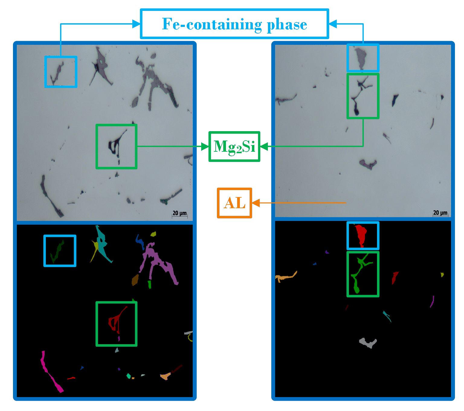
Datasets: In order to verify the proposed method, we built an experimental dataset, which contains 100 five-series aluminum alloy metallographic images. These aluminum alloy metallographic images were taken by a metallographic microscope and include three different types of phases, such as Mg2Si, aluminum and Fe-containing phase. The typical aluminum alloy metallographic images are shown in Figure 2. In this figure, the two images above are two typical aluminum alloy metallographic images, and the two images below are their ground truths. In the labelled images, we set aluminum as the background and labelled it in black. At the same time, we set microstructure as the object or foreground. It should be noted that in the semantic segmentation task, we labelled different instances of the same object with the same color. As opposed to the semantic segmentation, in the instance segmentation, we labelled different instances of the same object with different colors. For example, we labelled each instance microstructure with a different color, as shown in Figure 2.
Implementation details: In the experiments, we used the cross validation method to ensure the accuracy of the evaluation results. We divided dataset D into five mutually exclusive subsets with the same size, D = D 1 D 2 D 3 D 4 D 5 , and D i D j = where ( i j). We picked four subsets as the training set and the remaining subset as the test set, and then obtained five experimental results, as shown in the second to sixth columns in Table 1, Table 2, Table 3, Table 4, Table 5 and Table 6. In the process of training Mask R-CNN, we used a fixed learning rate γ 1 of 0.01, a momentum ψ 1 of 0.9 in SGD with momentum algorithm which can not only improve the training stability and accelerate the training process to certain extent, but also gives a certain ability to get rid of local optimum solution. In FPN, the backbone is Resnet101, the pyramid size is 256 and the strides are 4, 8, 16, 32 and 64. In RPN, the anchor stride is 1, the non-max suppression threshold is 0.7, the number of train anchors per image is 256, anchor ratios are 0.5, 1 and 2, and anchor scales are 32, 64, 128, 256 and 512. In R-CNN and FCN, the pool size is 7, the mask pool size is 14, the train ROI per image is 200, the ROI positive ratio is 0.33, the mask shape is 28 × 28 , the detection max instance is 100, the detection min confidence is 0.7 and the detection threshold is 0.3. The training process reaches its convergence when the epoch number κ 1 = 100 and each epoch contains 100 steps. By using the coco pre-training model to initialize network parameters, we made the model converge faster and obtained a better result. Moreover, the L 2 regularization was used, and the regularization coefficient λ = 0.0001 .

3.2. Evaluation Metrics

The aim of this section was to analyze the instance segmentation performance of the proposed method. Let D = I n , y n represent the test dataset and f θ represent our proposed method. We used six different evaluation metrics to evaluate this method, including Acc, Precision, Sn (Sensitivity, also named Recall), Sp (Specificity), IOU and F 1 . These metrics have been widely used in the literature. These six evaluation metrics are defined by the following formula:
(1) The Acc can be calculated by the following formula
A c c ( f θ ; D ) = T P + T N T P + T N + F P + F N ,
where TN is the number of true negatives, TP is the number of true positives, FN is the number of false negatives and FP is the number of false positives.
(2) The Precision is defined by
P r e c i s i o n ( f θ ; D ) = T P T P + F P .
(3) The Sn is defined by
S n ( f θ ; D ) = T N T N + F N .
(4) The Sp is defined by
S p ( f θ ; D ) = T N T N + F P .
(5) The IOU is defined by
I O U ( f θ ; D ) = T P T P + F N + F P .
(6) The F 1 is defined by
F 1 ( f θ ; D ) = 2 T P 2 T P + F N + F P .

3.3. Performance Comparison

(1) Quantitative performance comparison
In this experiment, we implemented five different mask loss functions on the basis of the proposed framework. For the easy description, we set f i ( i = 1 : 5 ) to denote the i-th method. The first method f 1 uses loss function L B C E . Similarly, f 2 uses loss function L D I C E , f 3 uses loss function L I o U , f 4 uses loss function L T v e r s k y , and f 5 uses loss function L S S . In addition, we show the quantitative comparison results of six different evaluation metrics, including Acc, Precision, Sn, Sp, IOU and F 1 .
In Table 1, the comparison results of Acc are shown. The first column denotes five different instance segmentation methods which were used in this experiment. The second to sixth columns show the results of five different cross experiments. The last column in the table shows the median of five experimental results. The first row denotes the experiment number. From these experimental results, we can see that the Acc of the five methods can be more than 99%. Therefore, from these experimental results, we can conclude that the five different instance segmentation methods implemented in our proposed framework can obtain a good segmentation performance. However, we can clearly observed that the distribution of this evaluation metric is very dense, so it is difficult to evaluate the performance of the metallographic image segmentation method. The main reason for this problem is that the proportion of target and background in metallographic image is too small.
Similarly, the comparison results of Sp are shown in Table 2. From these experimental results, we can see that the Sp of the five methods can reach up to more than 99%. Similarly to the Acc metric, this evaluation metric is also disturbed by background, so it cannot effectively evaluate the performance of the metallographic image segmentation method.
The comparison results of Precision are shown in Table 3. From these experimental results, we can see that the precision of the five methods can reach more than 60%. Therefore, from these experimental results, we can see that the proposed five different instance segmentation methods can obtain satisfactory segmentation results. This metric can avoid the interference caused by large background, so it is more suitable to evaluate the performance of the metallographic image segmentation method.
Similarly, the comparison results of Sn, IOU and F1 are shown in Table 4, Table 5 and Table 6, respectively. We can see that the Sn of the five methods can reach more than 62%, the IOU of the five methods can reach more than 53%, and the F1 of five methods can reach more than 61%. These three metrics can also effectively evaluate the performance of the metallographic image segmentation method. These experimental results verify the effectiveness of the proposed framework.
To sum up, we can obtain the following conclusions: (1) Acc and Sp evaluation metrics cannot effectively evaluate the performance of the metallographic image segmentation method. Instead, we can use Precision, Sn, IOU and F1 four evaluation metrics to effectively evaluate the performance of the metallographic image segmentation method. (2) The segmentation framework proposed in this paper can complete the task of instance segmentation and the five different methods based on the framework can achieve a satisfactory segmentation performance.
In addition, we show the box plot of the experiment results obtained by the five methods for six evaluation metrics. As shown in Figure 3 and Figure 4, the box plot is able to reflect the characteristics of the experimental data distribution. In the figures, from top to bottom, we can clearly observe the statistical characteristics of the experimental data, including upper extreme, upper quartile, median, lower quartile and lower extreme.
In Figure 3a, we show the box plot of Acc metric. The X-axis represents accuracy (Acc), and the Y-axis represents five different methods. From this figure, we can observe the following: (1) All median values are located between 0.999436 and 0.999551 and the length of the interval is less than 0.000115. (2) The experimental results are mainly distributed between 0.999270 and 0.999599 and the length of the interval is less than 0.000163. Therefore, we can conclude that these five methods can obtain a good segmentation performance. However, the performance of the segmentation algorithm cannot be evaluated effectively because the distribution of the metric values is too centralized.
In Figure 3b, we show the box plot of the specificity metric. The X-axis represents specificity(Sp) and the Y-axis represents the five different methods. From the figure, we can observe: (1) All median values are concentrated between 0.999601 and 0.999732, and the length of the interval is less than 0.000131. (2) The experimental results are mainly distributed between 0.999494 and 0.999882, and the length of the interval is less than 0.000388. Similarly to Acc, the distribution of metric value is too centralized, so it is not suitable to evaluate the performance of the segmentation method of the aluminum alloy metallographic image.
In Figure 3c, we show the box plot of the precision metric. The X-axis represents precision, and the Y-axis represents the five different methods. From the figure, we can observe the following: (1) All median values are concentrated between 0.633345 and 0.676730, and the length of the interval is less than 0.043385. (2) The experimental results are mainly distributed between 0.590931 and 0.764655, and the length of the interval is less than 0.173724. Therefore, we can conclude that these five methods can get good segmentation performance and that this metric can be used to evaluate the performance of the aluminum alloy metallographic image segmentation method.
Figure 4a shows the box plot of the sensitivity metric. We can observe: (1) All median values are concentrated between 0.658808 and 0.690875, and the length of the interval is less than 0.032067. (2) The experimental results are mainly distributed between 0.624957 and 0.756356, and the length of the interval is less than 0.131399. Therefore, we can conclude that the proposed segmentation framework of the aluminum alloy metallographic image has a satisfactory robustness.
In Figure 4b, we show the box plot of the IOU metric. From the figure, we can observe: (1) All median values are concentrated between 0.572862 and 0.590477, and the length of the interval is less than 0.017615. (2) The experimental results are mainly distributed between 0.537472 and 0.653169, and the length of the interval is less than 0.115697. We can find that these five methods can obtain a good segmentation performance.
In Figure 4c, we show the box plot of F1 metric. From this figure, we can observe: (1) All median values are concentrated between 0.648007 and 0.663737, and the length of the interval is less than 0.01573. (2) The experimental results are mainly distributed between 0.611533 and 0.737506, and the length of the interval is less than 0.125973. We can find that these five methods can get good segmentation performance. Similarly, we can conclude that the proposed segmentation framework of aluminum alloy metallographic image has satisfactory robustness.
In summary, we can make the following conclusions: (1) The proposed segmentation framework of a aluminum alloy metallographic image can effectively achieve the task of instance segmentation and five different methods based on this framework can obtain a satisfactory segmentation result. (2) The distributions of Acc and specificity metric values are too centralized so they are not suitable to evaluate the performance of the aluminum alloy metallographic image segmentation method. Instead, the Precision, Sn, IOU and F1 four evaluation metrics are suitable to evaluate the performance of segmentation method of the aluminum alloy metallographic image.
(2) Qualitative performance comparison
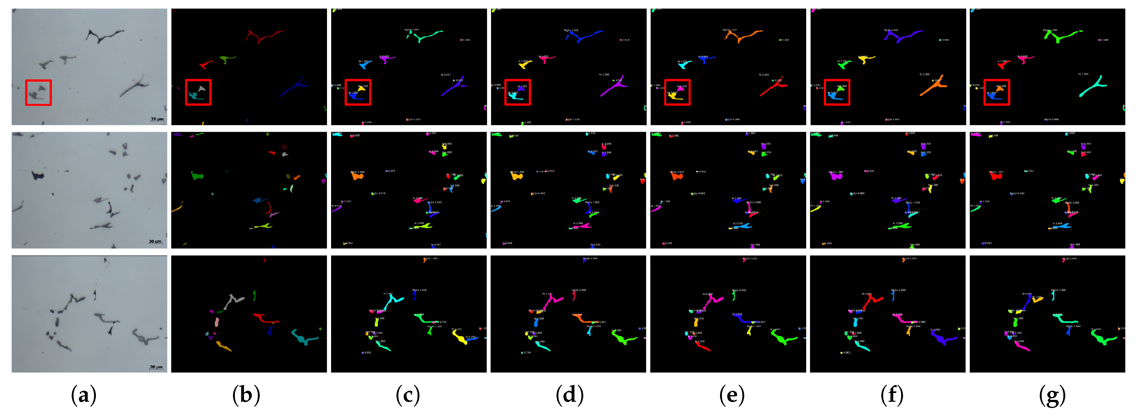
To further evaluate the proposed instance segmentation framework of metallographic image, Figure 5 shows the qualitative performance comparison among the five different methods implemented in this framework, including the binary cross-entropy loss ( f 1 ), Dice loss ( f 2 ), IoU loss ( f 3 ), Tversky loss ( f 4 ) and SS loss ( f 5 ). Three original metallographic images are shown in Figure 5a and their corresponding ground truth results are shown in Figure 5b. In the ground truth, the Aluminum is represented in black, and the other instances of microstructure are represented in different colors. The instance segmentation results of the five different methods are shown in Figure 5c–g. From these results, we can observe that these five methods can accomplish the task of instance segmentation of microstructure in a metallographic image.
For convenient observation, Figure 6 shows the local enlarged maps of instance segmentation results obtained by the five proposed methods, including the binary cross-entropy loss ( f 1 ), Dice loss ( f 2 ), IoU loss ( f 3 ), Tversky loss ( f 4 ) and SS loss ( f 5 ). The original local enlarged map is shown in Figure 6a and the corresponding ground truth is shown in Figure 6b.
In these local enlarged maps, we can see two instances of the Fe-containing phase. As opposed to semantic segmentation, the instance segmentation method proposed in this paper can not only segment different microstructures, but also segment different instances in the microstructure. As shown in Figure 6, we segmented different instances of the Fe-containing phase and marked them with different colors. From these experimental results, we can conclude that the instance segmentation methods proposed in this paper can achieve a satisfactory segmentation performance.
The proposed instance segmentation framework can automatically realize the representation learning of different metal alloys by using the given samples. We do not need to design features manually for different segmentation objects. Therefore, this instance segmentation framework can also be used for other types of metal alloys. In addition, for the proposed instance segmentation framework, the discriminability of the object instance has an important impact on the segmentation performance. When the phases of a given metal alloy have a stronger discriminability, this framework can obtain better instance segmentation results.

3.4. Convergence Analysis

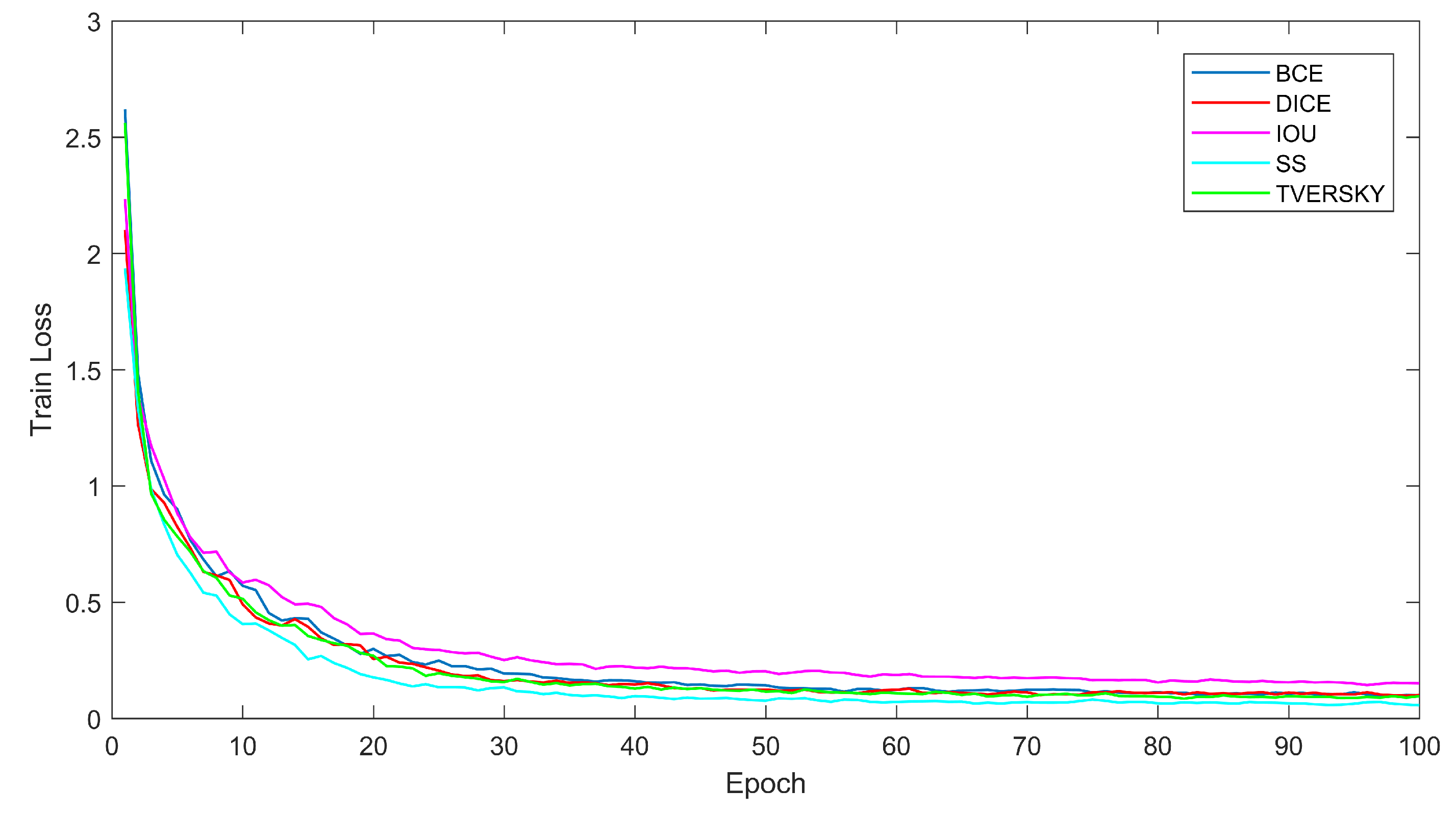
The aim of this experiment was to analyze the convergence of the proposed framework. The loss curves with time for five different methods are shown in Figure 7. From the Figure 7, we can observe that these five methods can converge and the methods f 5 have a better convergence speed than the other methods. This verifies the convergence of the proposed instance segmentation framework.

4. Conclusions

A new metallographic image segmentation framework is proposed, which can achieve the task of automatic instance segmentation for aluminum alloy metallographic images. This segmentation framework provides a powerful tool for the quantitative analysis of metallographic images. Based on this proposed framework, we implemented five different instance segmentation methods by using different loss functions. A large number of experimental results verified the effectiveness of the proposed method. In order to evaluate the performance of the metallographic image segmentation method effectively, we compared and analyzed six typical segmentation performance evaluation metrics, including Accuracy, Precision, Sensitivity, Specificity, IOU and F 1 measure. From the experimental results, we found that Precision, Specificity, IOU and F 1 measure can effectively evaluate the performance of metallographic image segmentation methods. In the future, we plan to investigate the use of weakly supervised learning methods for dealing with the problem of insufficiency in high-quality hand-labeled data samples.

Author Contributions

Conceptualization, D.C. and D.G.; methodology, D.C. and D.G.; software, D.G.; validation, D.G. and F.L.; formal analysis, D.C.; investigation, D.C. and D.G.; resources, S.L.; data curation, D.G. and F.L.; writing—original draft preparation, D.C.; writing—review and editing, D.C. and D.G.; visualization, D.G.; supervision, S.L. and F.L. All authors have read and agreed to the published version of the manuscript.

Funding

This research was funded in part by the National Key R&D Program of China under Grant 2017YFB0306400 and National Natural Science Foundation of China under Grant 61773104.

Conflicts of Interest

The authors declare no conflict of interest.

References

  1. Heinz, A.; Haszler, A.; Keidel, C.; Moldenhauer, S.; Benedictus, R.; Miller, W. Recent development in aluminium alloys for aerospace applications. Mater. Sci. Eng. A 2000, 280, 102–107. [Google Scholar] [CrossRef]
  2. Hirsch, J.; Al-Samman, T. Superior light metals by texture engineering: Optimized aluminum and magnesium alloys for automotive applications. Acta Mater. 2013, 61, 818–843. [Google Scholar] [CrossRef]
  3. Martin, J.H.; Yahata, B.D.; Hundley, J.M.; Mayer, J.A.; Schaedler, T.A.; Pollock, T.M. 3D printing of high-strength aluminium alloys. Nature 2017, 549, 365. [Google Scholar] [CrossRef] [PubMed]
  4. Zhang, J.; Song, B.; Wei, Q.; Bourell, D.; Shi, Y. A review of selective laser melting of aluminum alloys: Processing, microstructure, property and developing trends. J. Mater. Sci. Technol. 2019, 35, 270–284. [Google Scholar] [CrossRef]
  5. Roy, N.; Samuel, A.; Samuel, F. Porosity formation in AI-9 Wt pct Si-3 Wt pct Cu alloy systems: Metallographic observations. Metall. Mater. Trans. A 1996, 27, 415–429. [Google Scholar] [CrossRef]
  6. Rajasekhar, K.; Harendranath, C.; Raman, R.; Kulkarni, S. Microstructural evolution during solidification of austenitic stainless steel weld metals: A color metallographic and electron microprobe analysis study. Mater. Charact. 1997, 38, 53–65. [Google Scholar] [CrossRef]
  7. Girault, E.; Jacques, P.; Harlet, P.; Mols, K.; Van Humbeeck, J.; Aernoudt, E.; Delannay, F. Metallographic methods for revealing the multiphase microstructure of TRIP-assisted steels. Mater. Charact. 1998, 40, 111–118. [Google Scholar] [CrossRef]
  8. Rohatgi, A.; Vecchio, K.; Gray Iii, G. A metallographic and quantitative analysis of the influence of stacking fault energy on shock-hardening in Cu and Cu–Al alloys. Acta Mater. 2001, 49, 427–438. [Google Scholar] [CrossRef]
  9. Moreira, F.; Xavier, F.; Gomes, S.; Santos, J.; Freitas, F.; Freitas, R. New analysis method application in metallographic images through the construction of mosaics via speeded up robust features and scale invariant feature transform. Materials 2015, 8, 3864–3882. [Google Scholar]
  10. Povstyanoi, O.Y.; Sychuk, V.; McMillan, A.; Zabolotnyi, O. Metallographic analysis and microstructural image processing of sandblasting nozzles produced by powder metallurgy methods. Powder Metall. Metal Ceram. 2015, 54, 234–240. [Google Scholar] [CrossRef]
  11. Chowdhury, A.; Kautz, E.; Yener, B.; Lewis, D. Image driven machine learning methods for microstructure recognition. Comput. Mater. Sci. 2016, 123, 176–187. [Google Scholar] [CrossRef] [Green Version]
  12. Campbell, A.; Murray, P.; Yakushina, E.; Marshall, S.; Ion, W. New methods for automatic quantification of microstructural features using digital image processing. Mater. Design 2018, 141, 395–406. [Google Scholar] [CrossRef] [Green Version]
  13. Zhenying, X.; Jiandong, Z.; Qi, Z.; Yamba, P. Algorithm based on regional separation for automatic grain boundary extraction using improved mean shift method. Surf. Topogr. Metrol. Prop. 2018, 6, 025001. [Google Scholar] [CrossRef]
  14. Journaux, S.; Gouton, P.; Paindavoine, M.; Thauvin, G. Evaluating creep in metals by grain boundary extraction using directional wavelets and mathematical morphology. Revue de Métall. Int. J. Metall. 2001, 98, 485–499. [Google Scholar] [CrossRef]
  15. Sun, Q.D.; Gao, S.F.; Huang, J.W.; Chen, W. Metallographical Image Segmentation and Compression. In Applied Mechanics and Materials; Trans Tech Publications Ltd.: Bäch SZ, Switzerland, 2012; Volume 152, pp. 276–280. [Google Scholar]
  16. Simmons, J.; Przybyla, C.; Bricker, S.; Kim, D.W.; Comer, M. Physics of MRF regularization for segmentation of materials microstructure images. In Proceedings of the 2014 IEEE International Conference on Image Processing (ICIP), Paris, France, 27–30 October 2014; pp. 4882–4886. [Google Scholar]
  17. Cheng, H.C.; Cardone, A.; Varshney, A. Interactive exploration of microstructural features in gigapixel microscopy images. In Proceedings of the 2017 IEEE International Conference on Image Processing (ICIP), Beijing, China, 17–20 September 2017; pp. 335–339. [Google Scholar]
  18. Chen, L.; Han, Y.; Cui, B.; Guan, Y.; Luo, Y. Two-dimensional fuzzy clustering algorithm (2DFCM) for metallographic image segmentation based on spatial information. In Proceedings of the 2015 2nd International Conference on Information Science and Control Engineering, Shanghai, China, 24–26 April 2015; pp. 519–521. [Google Scholar]
  19. De Albuquerque, V.H.C.; de Alexandria, A.R.; Cortez, P.C.; Tavares, J.M.R. Evaluation of multilayer perceptron and self-organizing map neural network topologies applied on microstructure segmentation from metallographic images. NDT E Int. 2009, 42, 644–651. [Google Scholar] [CrossRef]
  20. Bulgarevich, D.S.; Tsukamoto, S.; Kasuya, T.; Demura, M.; Watanabe, M. Pattern recognition with machine learning on optical microscopy images of typical metallurgical microstructures. Sci. Rep. 2018, 8, 2078. [Google Scholar] [CrossRef] [PubMed]
  21. Papa, J.P.; Nakamura, R.Y.; De Albuquerque, V.H.C.; Falcão, A.X.; Tavares, J.M.R. Computer techniques towards the automatic characterization of graphite particles in metallographic images of industrial materials. Expert Syst. Appl. 2013, 40, 590–597. [Google Scholar] [CrossRef]
  22. De Albuquerque, V.H.C.; Silva, C.C.; Menezes, T.I.D.S.; Farias, J.P.; Tavares, J.M.R. Automatic evaluation of nickel alloy secondary phases from SEM images. Microsc. Res. Tech. 2011, 74, 36–46. [Google Scholar] [CrossRef]
  23. DeCost, B.L.; Holm, E.A. A computer vision approach for automated analysis and classification of microstructural image data. Comput. Mater. Sci. 2015, 110, 126–133. [Google Scholar] [CrossRef] [Green Version]
  24. Gola, J.; Britz, D.; Staudt, T.; Winter, M.; Schneider, A.S.; Ludovici, M.; Mücklich, F. Advanced microstructure classification by data mining methods. Comput. Mater. Sci. 2018, 148, 324–335. [Google Scholar] [CrossRef]
  25. LeCun, Y.; Bengio, Y.; Hinton, G. Deep learning. Nature 2015, 521, 436–444. [Google Scholar] [CrossRef] [PubMed]
  26. Goodfellow, I.; Bengio, Y.; Courville, A. Deep Learning; MIT Press: Cambridge, MA, USA, 2016. [Google Scholar]
  27. Sanchez-Lengeling, B.; Aspuru-Guzik, A. Inverse molecular design using machine learning: Generative models for matter engineering. Science 2018, 361, 360–365. [Google Scholar] [CrossRef] [PubMed] [Green Version]
  28. Azimi, S.M.; Britz, D.; Engstler, M.; Fritz, M.; Mücklich, F. Advanced steel microstructural classification by deep learning methods. Sci. Rep. 2018, 8, 2128. [Google Scholar] [CrossRef] [PubMed]
  29. Ma, B.; Ban, X.; Huang, H.; Chen, Y.; Liu, W.; Zhi, Y. Deep learning-based image segmentation for al-la alloy microscopic images. Symmetry 2018, 10, 107. [Google Scholar] [CrossRef] [Green Version]
  30. Chen, H.; Qi, X.; Yu, L.; Dou, Q.; Qin, J.; Heng, P.A. DCAN: Deep contour-aware networks for object instance segmentation from histology images. Med. Image Anal. 2017, 36, 135–146. [Google Scholar] [CrossRef] [PubMed]
  31. Yi, J.; Wu, P.; Jiang, M.; Huang, Q.; Hoeppner, D.J.; Metaxas, D.N. Attentive neural cell instance segmentation. Med. Image Anal. 2019, 55, 228–240. [Google Scholar] [CrossRef]
  32. De Bel, T.; Hermsen, M.; Litjens, G.; van der Laak, J. Structure Instance Segmentation in Renal Tissue: A Case Study on Tubular Immune Cell Detection. In Computational Pathology and Ophthalmic Medical Image Analysis; Springer: Berlin, Germany, 2018; pp. 112–119. [Google Scholar]
  33. Guerrero-Pena, F.A.; Fernandez, P.D.M.; Ren, T.I.; Yui, M.; Rothenberg, E.; Cunha, A. Multiclass weighted loss for instance segmentation of cluttered cells. In Proceedings of the 2018 25th IEEE International Conference on Image Processing (ICIP), Athens, Greece, 7–10 October 2018; pp. 2451–2455. [Google Scholar]
  34. Mou, L.; Zhu, X.X. Vehicle instance segmentation from aerial image and video using a multitask learning residual fully convolutional network. IEEE Trans. Geosci. Remote Sens. 2018, 56, 6699–6711. [Google Scholar] [CrossRef] [Green Version]
  35. He, K.; Gkioxari, G.; Dollár, P.; Girshick, R. Mask r-cnn. In Proceedings of the IEEE International Conference on Computer Vision, Venice, Italy, 22–29 October 2017; pp. 2961–2969. [Google Scholar]
  36. Milletari, F.; Navab, N.; Ahmadi, S.A. V-net: Fully convolutional neural networks for volumetric medical image segmentation. In Proceedings of the 2016 Fourth International Conference on 3D Vision (3DV), Stanford, CA, USA, 25–28 October 2016; pp. 565–571. [Google Scholar]
  37. Rahman, M.A.; Wang, Y. Optimizing intersection-over-union in deep neural networks for image segmentation. In Proceedings of the International Symposium on Visual Computing, Las Vegas, NV, USA, 12–14 December 2016; pp. 234–244. [Google Scholar]
  38. Salehi, S.S.M.; Erdogmus, D.; Gholipour, A. Tversky loss function for image segmentation using 3D fully convolutional deep networks. In Proceedings of the International Workshop on Machine Learning in Medical Imaging, Quebec, QC, Canada, 10 September 2017; pp. 379–387. [Google Scholar]
  39. Brosch, T.; Yoo, Y.; Tang, L.Y.; Li, D.K.; Traboulsee, A.; Tam, R. Deep convolutional encoder networks for multiple sclerosis lesion segmentation. In Proceedings of the International Conference on Medical Image Computing and Computer-Assisted Intervention, Munich, Germany, 5–9 October 2015; pp. 3–11. [Google Scholar]
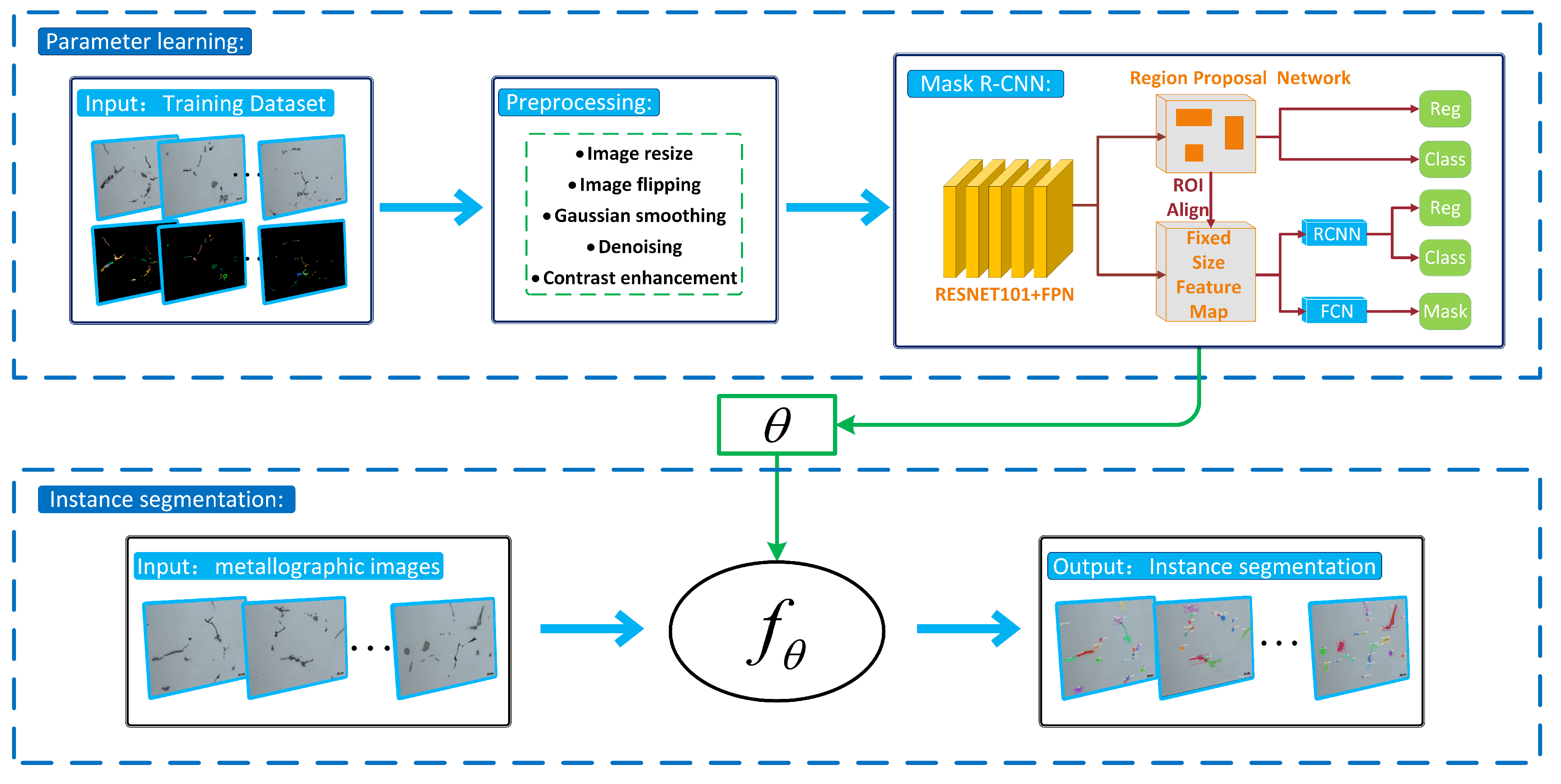
Figure 1. The flowchart of the proposed method.
Symmetry 12 00639 g001
Figure 2. Aluminum alloy metallographic image and ground truth.
Symmetry 12 00639 g002
Figure 3. The box plot of experimental results obtained by the five methods: (a) Accuracy; (b) Specificity; (c) Precision.
Symmetry 12 00639 g003
Figure 4. The box plot of experimental results obtained by the five methods: (a) Sensitivity; (b) IOU; (c) F1 Measure.
Symmetry 12 00639 g004
Figure 5. Qualitative performance comparison among the five different methods: (a) original image; (b) Ground truth; (c) Binary cross-entropy loss f 1 ; (d) Dice loss f 2 ; (e) IoU loss f 3 ; (f) Tversky loss f 4 ; (g) SS loss f 5 .
Symmetry 12 00639 g005
Figure 6. The local enlarged maps of instance segmentation results obtained by different methods (the “fe 1.000” inside the picture means the probability of this region being classified as Fe-containing phase is 1.000): (a) original image; (b) Ground truth; (c) Binary cross-entropy loss f 1 ; (d) Dice loss f 2 ; (e) IoU loss f 3 ; (f) Tversky loss f 4 ; (g) SS loss f 5 .
Symmetry 12 00639 g006
Figure 7. The loss curves for five different methods.
Symmetry 12 00639 g007
Table 1. The Acc comparison among the five different methods.
Acc12345Median
f 1 0.9995550.9994330.9994630.9995510.9995990.999551
f 2 0.9995510.9993640.9994950.9995060.9995250.999506
f 3 0.9995190.9993660.9995060.9995510.9995190.999519
f 4 0.9994360.9992770.9994110.9995320.9995050.999436
f 5 0.9994710.9992700.9994500.9995350.9995460.999471
Table 2. The Sp comparison among the five different methods.
SP12345Median
f 1 0.9997320.9996830.9996560.9998820.9998330.999732
f 2 0.9997230.9996090.9997080.9998340.9997600.999723
f 3 0.9997000.9996110.9997140.9998370.9997480.999714
f 4 0.9996010.9995030.9995790.9997590.9997060.999601
f 5 0.9996280.9994940.9996330.9997570.9997430.999633
Table 3. The precision comparison among the five different methods.
Precision12345Median
f 1 0.6494820.6536780.6630110.7572760.7646550.663011
f 2 0.6468590.6424320.6593440.7403310.7552420.659344
f 3 0.6451980.6488850.6767300.7474580.7369090.676730
f 4 0.6085180.6118370.6333450.7257100.7118290.633345
f 5 0.6254380.5909310.6348940.7395200.7250180.634894
Table 4. The Sn comparison among the five different methods.
SN12345Median
f 1 0.6308250.6390660.6776100.6695180.7117010.669518
f 2 0.6373240.6339610.6851010.6778320.6960870.677832
f 3 0.6249570.6316850.6588080.6898060.6958270.658808
f 4 0.6419410.6611900.6908750.7480320.7336680.690875
f 5 0.6676520.6418280.6704560.7462070.7563560.670456
Table 5. The IOU comparison among the five different methods.
IOU12345Median
f 1 0.5628090.5640190.5904770.6187160.6486130.590477
f 2 0.5641720.5572460.5889990.6189480.6325800.588999
f 3 0.5563830.5590840.5849600.6288080.6278910.584960
f 4 0.5498270.5548910.5799450.6466440.6360550.579945
f 5 0.5677110.5374720.5728620.6511920.6531690.572862
Table 6. THE F1 COMPARISON AMONG THE FIVE DIFFERENT METHODS.
F112345Median
f 1 0.6361200.6419560.6662170.7057930.7335400.666217
f 2 0.6386240.6338690.6674500.7029970.7200670.667450
f 3 0.6310620.6357870.6637370.7129350.7119420.663737
f 4 0.6213410.6315400.6572200.7316350.7184880.657220
f 5 0.6420510.6115330.6480070.7375060.7366520.648007