A Confrontation Decision-Making Method with Deep Reinforcement Learning and Knowledge Transfer for Multi-Agent System

Abstract
1. Introduction
1.1. Reinforcement Learning
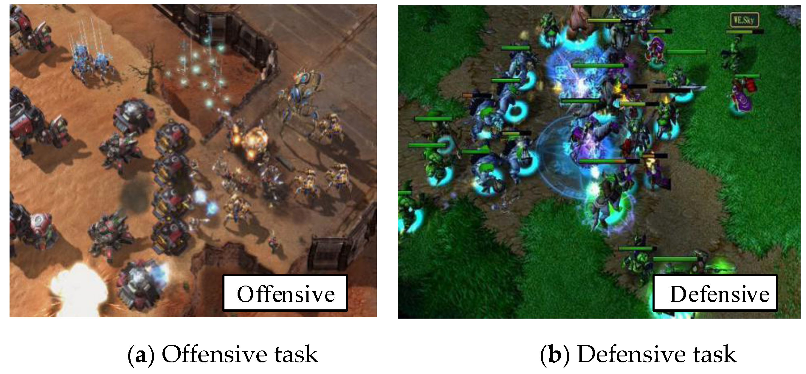
1.2. Multi-Agent Confrontation in the Real-Time Strategy Game
1.3. Confrontation Decision-Making with Reinforcement Learning for Multi-Agent System
1.4. Deep Reinforcement Learning
1.5. Knowledge Transfer
1.6. Contributions in This Work
1.7. Paper Structure
2. Background
2.1. Reinforcement Learning
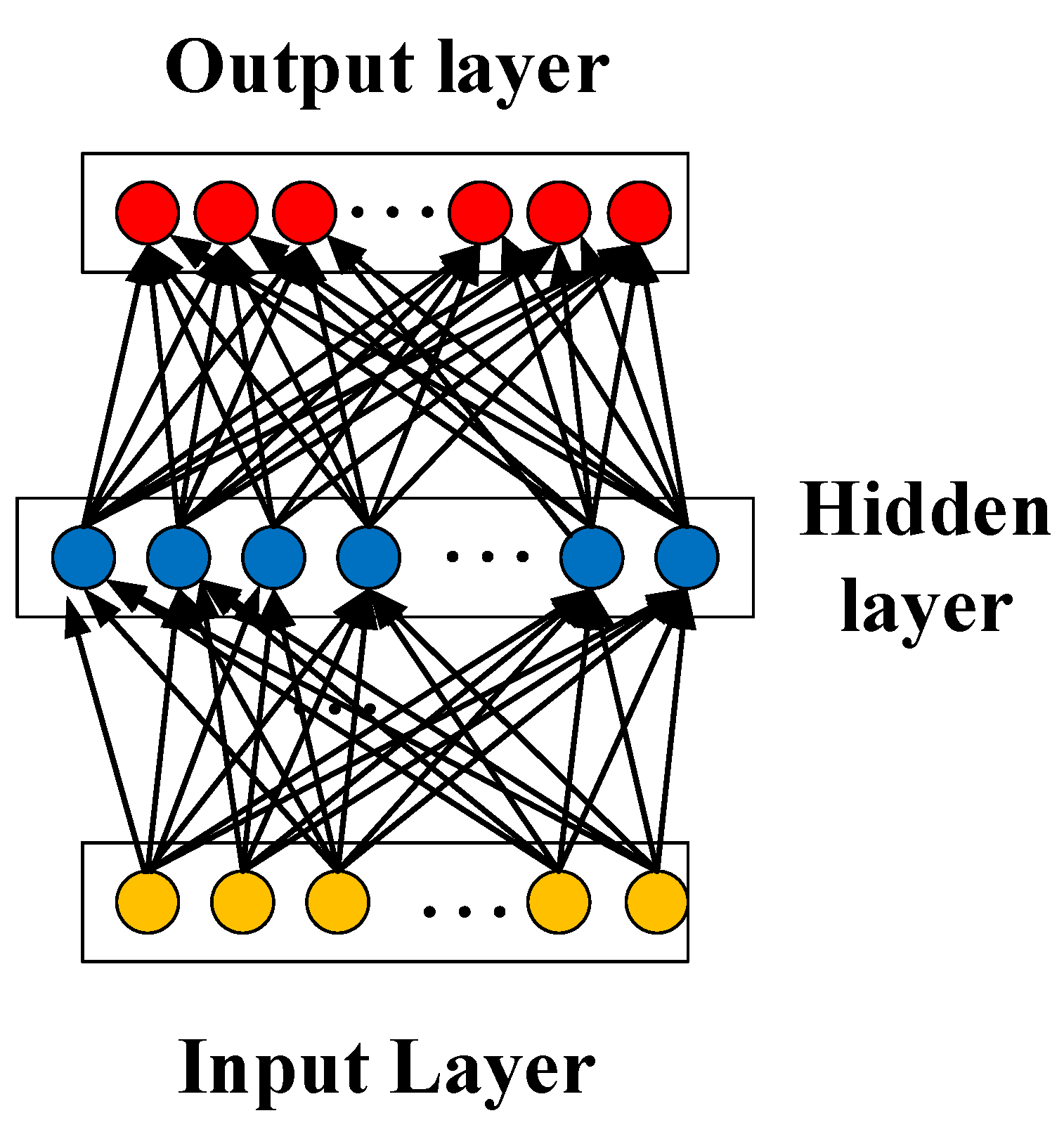
2.2. Neural Network
3. Description of Continuous Control Problem and a Classical Method
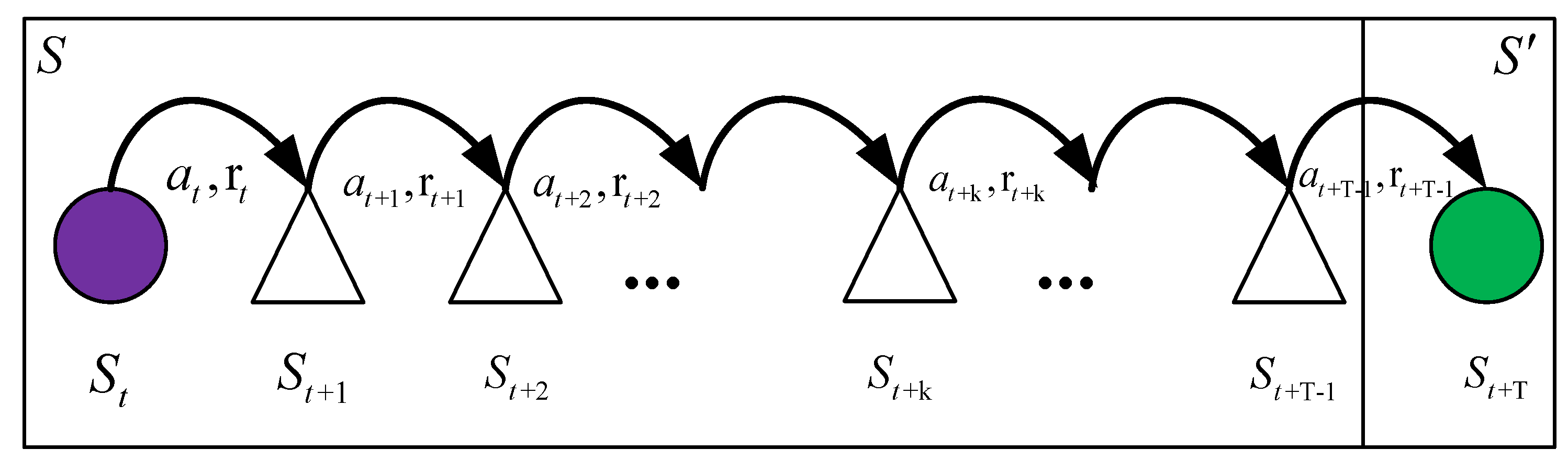
3.1. Optimal Control Problem Using Value Function in SMDPs Process
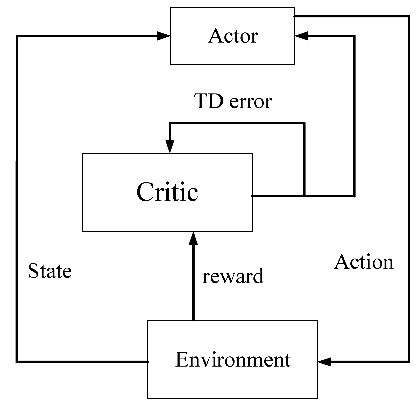
3.2. Classical Method for Optimal Control Using Actor–Critic
| Algorithm 1: Basic Procedure for Actor–Critic Algorithm |
|
4. Multi-Agent DDPG Algorithm with an Auxiliary Controller for Confrontation Decision-Making
4.1. Back Propagation Algorithm with a Momentum Mechanism
| Algorithm 2: Procedure for the Back-Propagation Algorithm with Momentum |
|
4.2. Multi-Agent DDPG Algorithm with Parameter Sharing
| Algorithm 3: Multi-Agent DDPG Algorithm with Parameter Sharing |
| Initialization: |
| Initialize the current network for the critic , using ; Initializes the current network for actor using . |
| Initialize the target networks for the critic and actor: , |
| Initialize the sampling pool For each agent =1, K do |
| For episode = 1, do |
| Initialize a random noise ; |
| Get the current state |
| For , do |
| , Perform action and observe the next state. , ; |
| Randomly select samples from the sampling pool ; |
| Update the parameters of the current network with momentum mechanism for critic using the Loss function: ; |
| Update the parameters of the current network with momentum mechanism for actor using : |
| Update target networks for the actor and the critic separately: , ; |
| End for End for |
| End for |
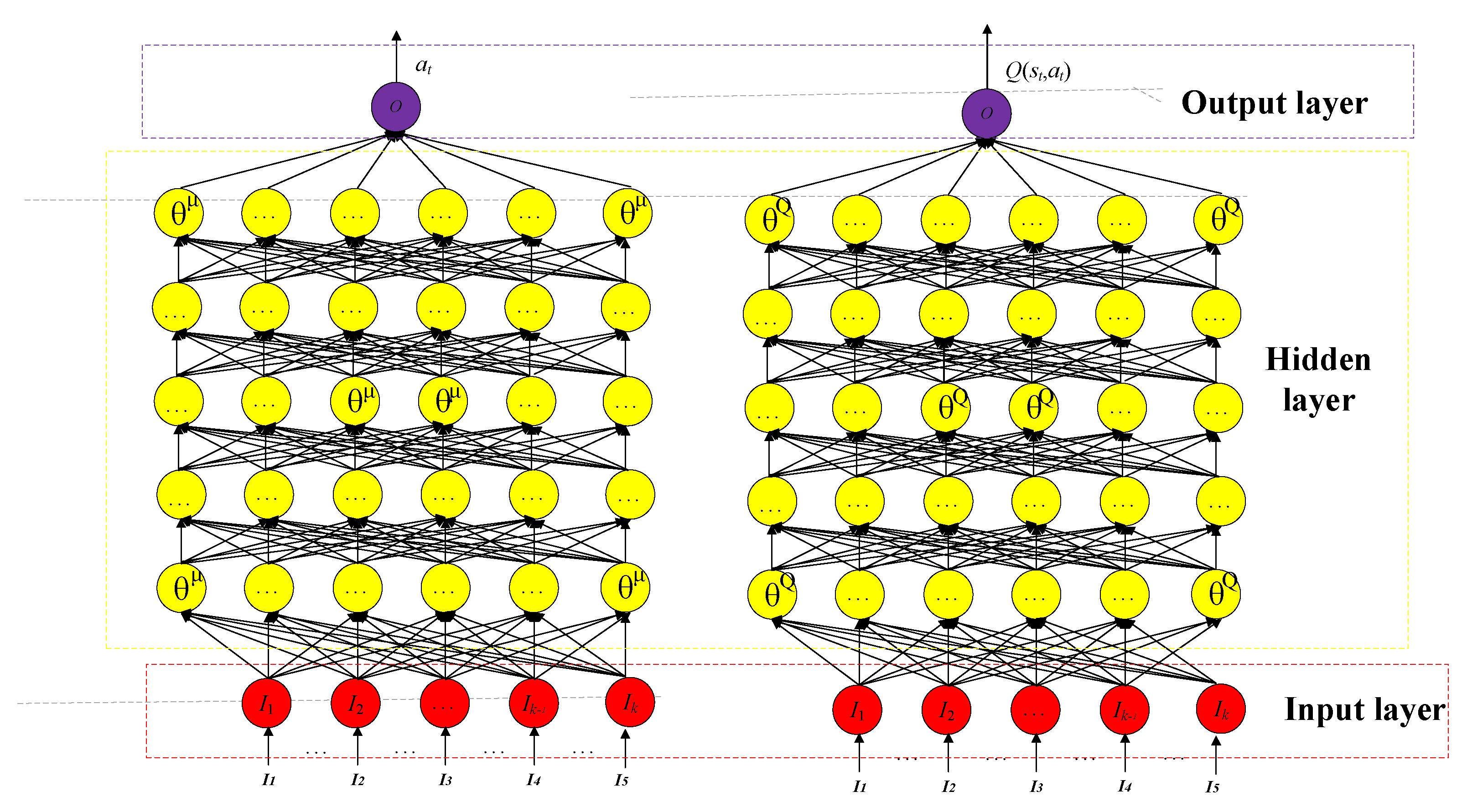
4.3. Neural Network Structure for the DDPG Algorithm
4.4. An Auxiliary Controller Using a Policy-Based RL Method
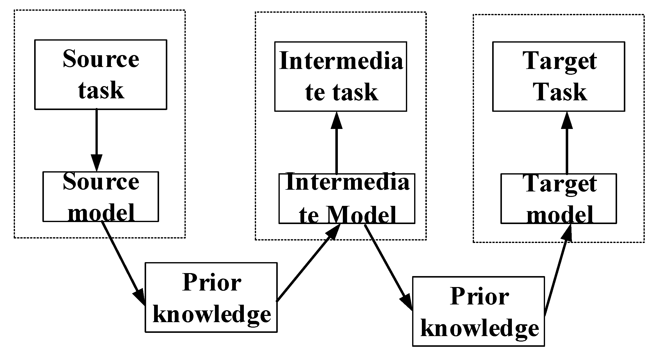
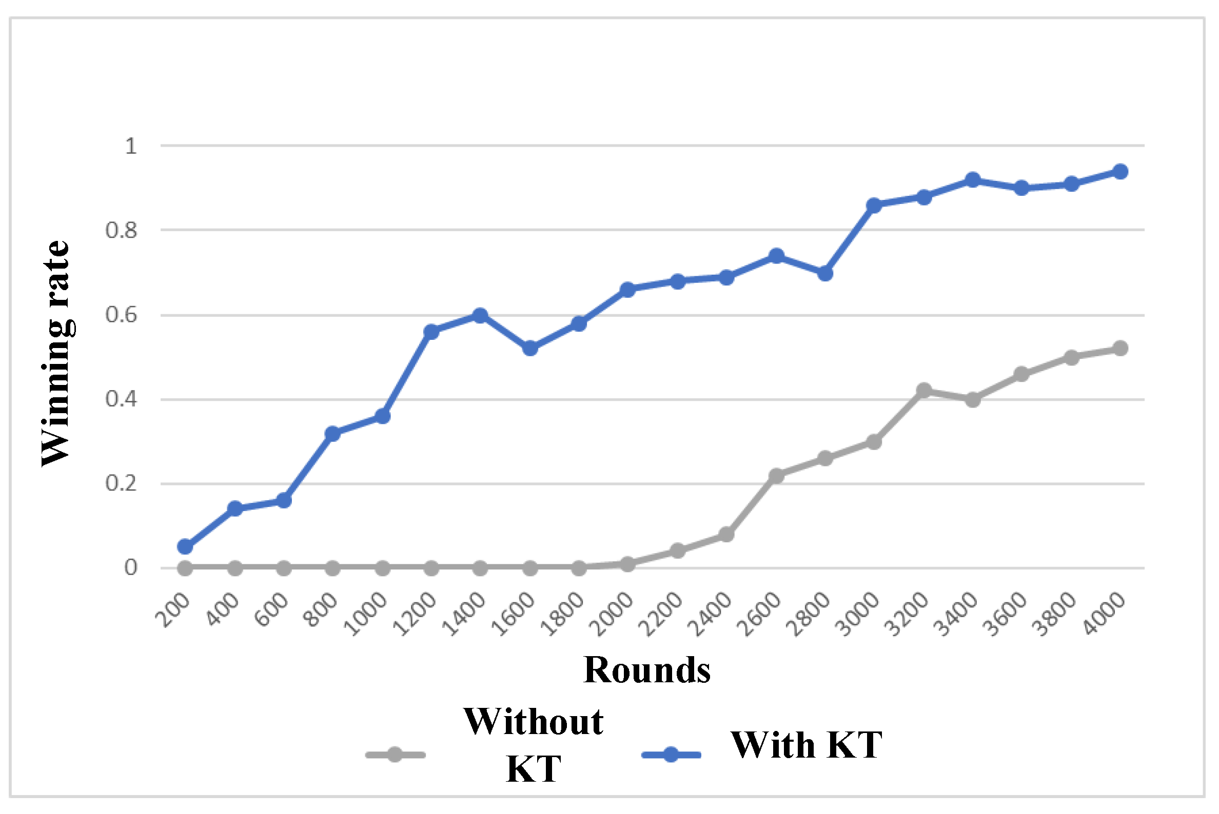
5. Knowledge Transfer Method
6. Effect Test for the Proposed Policy-Based RL Method
7. Experiment on StarCraft Task
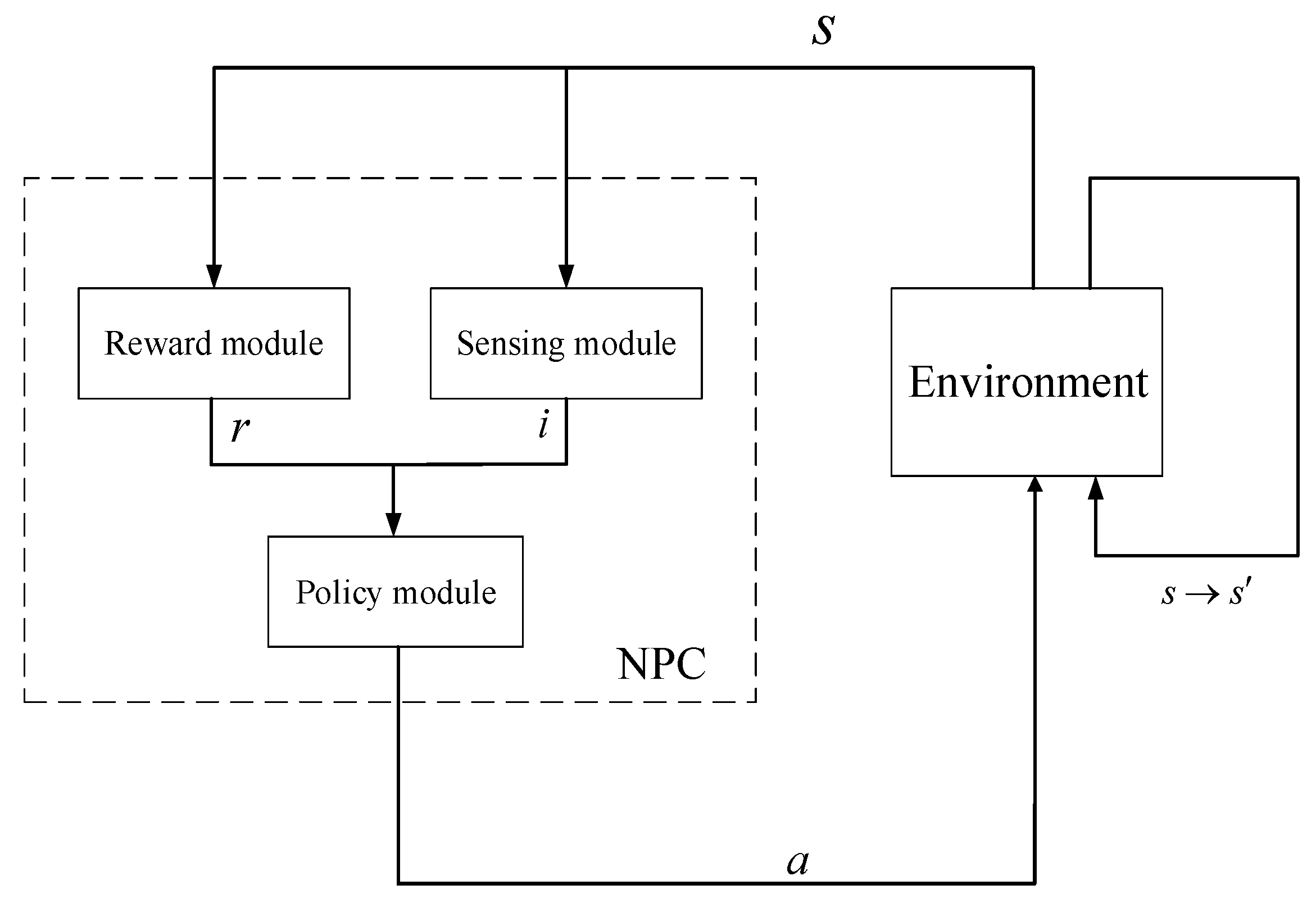
7.1. Reinforcement Learning Model for StarCraft Task
7.2. Experimental Configuration
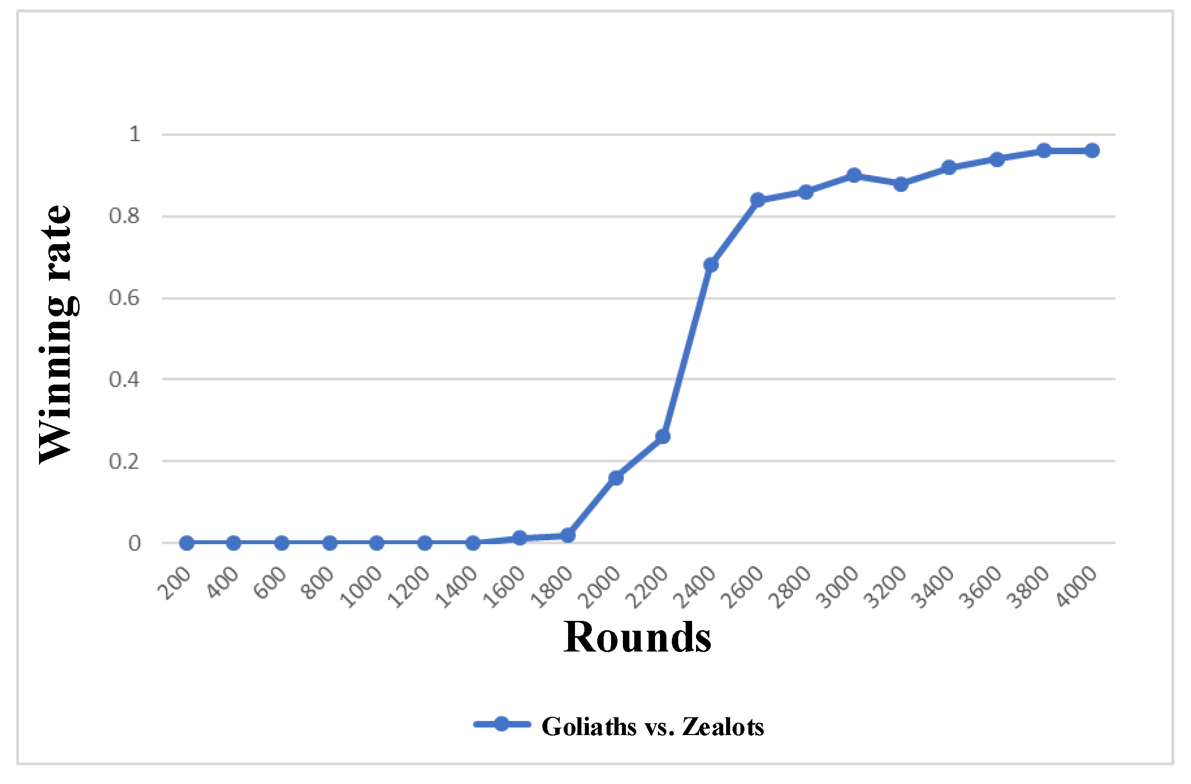
7.3. Confrontation Task-Goliaths vs. Zealots
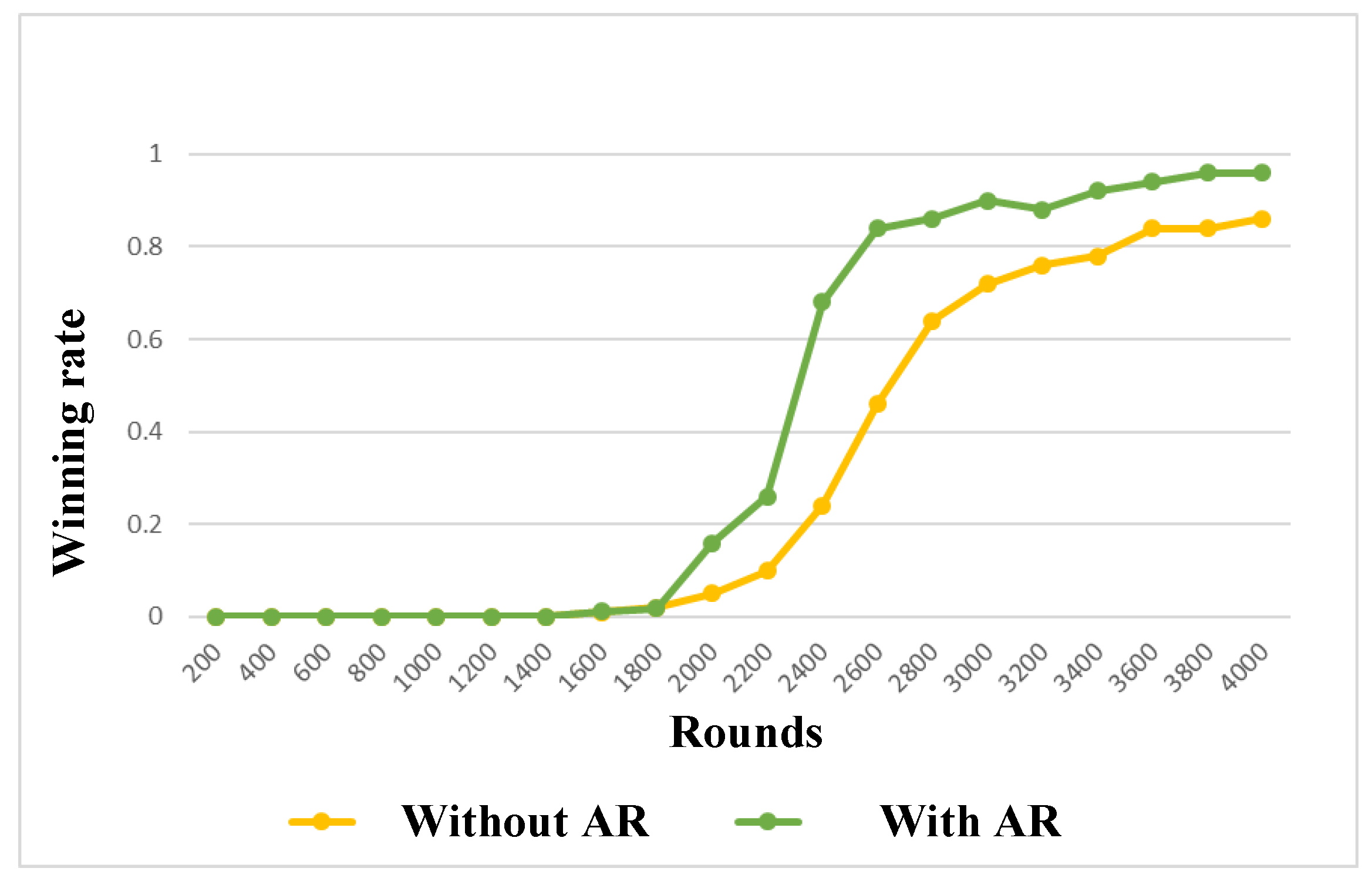
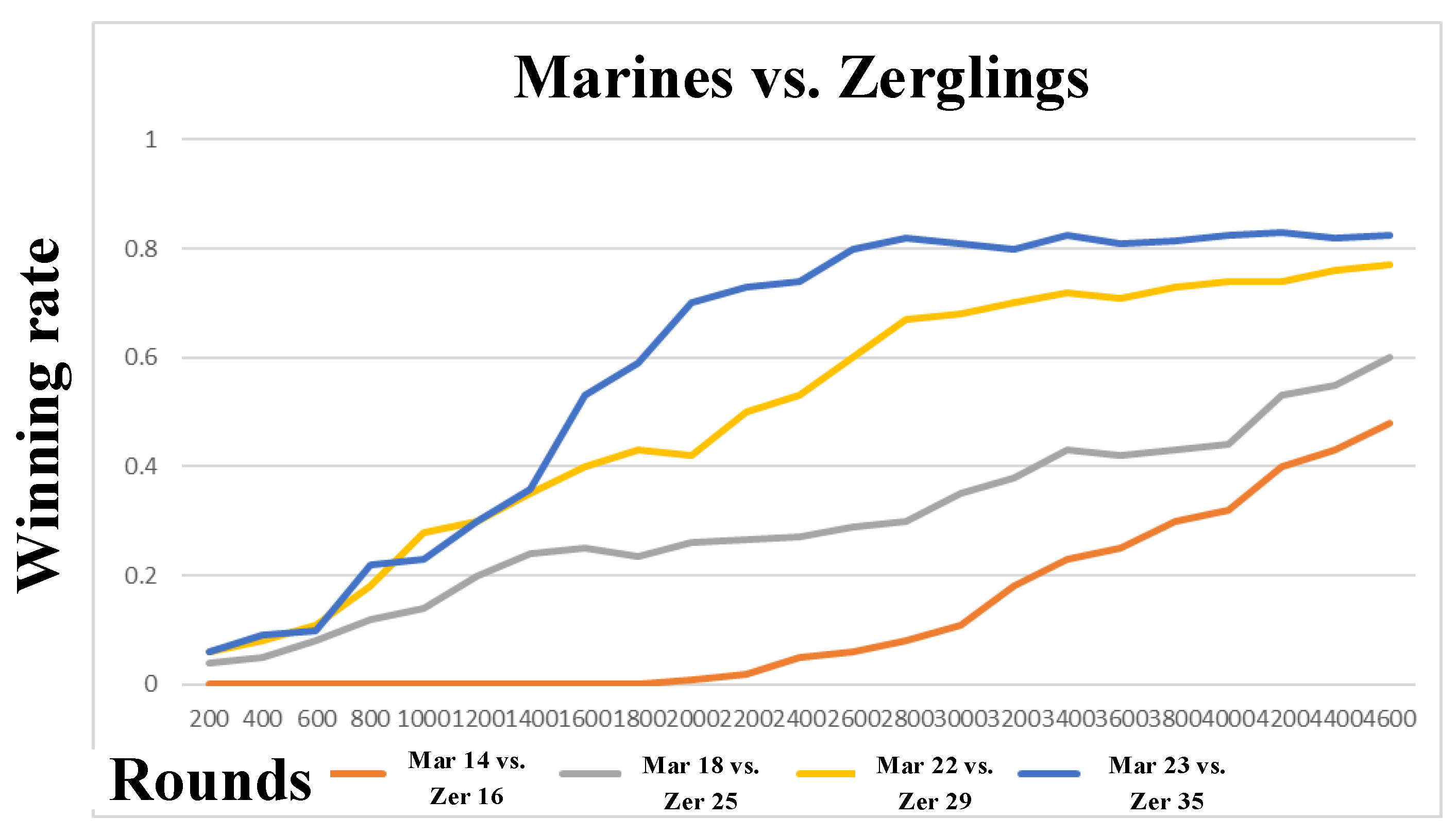
7.4. Confrontation Task-Goliaths vs. Zerglings
7.5. Large Scale Confrontation Scenario
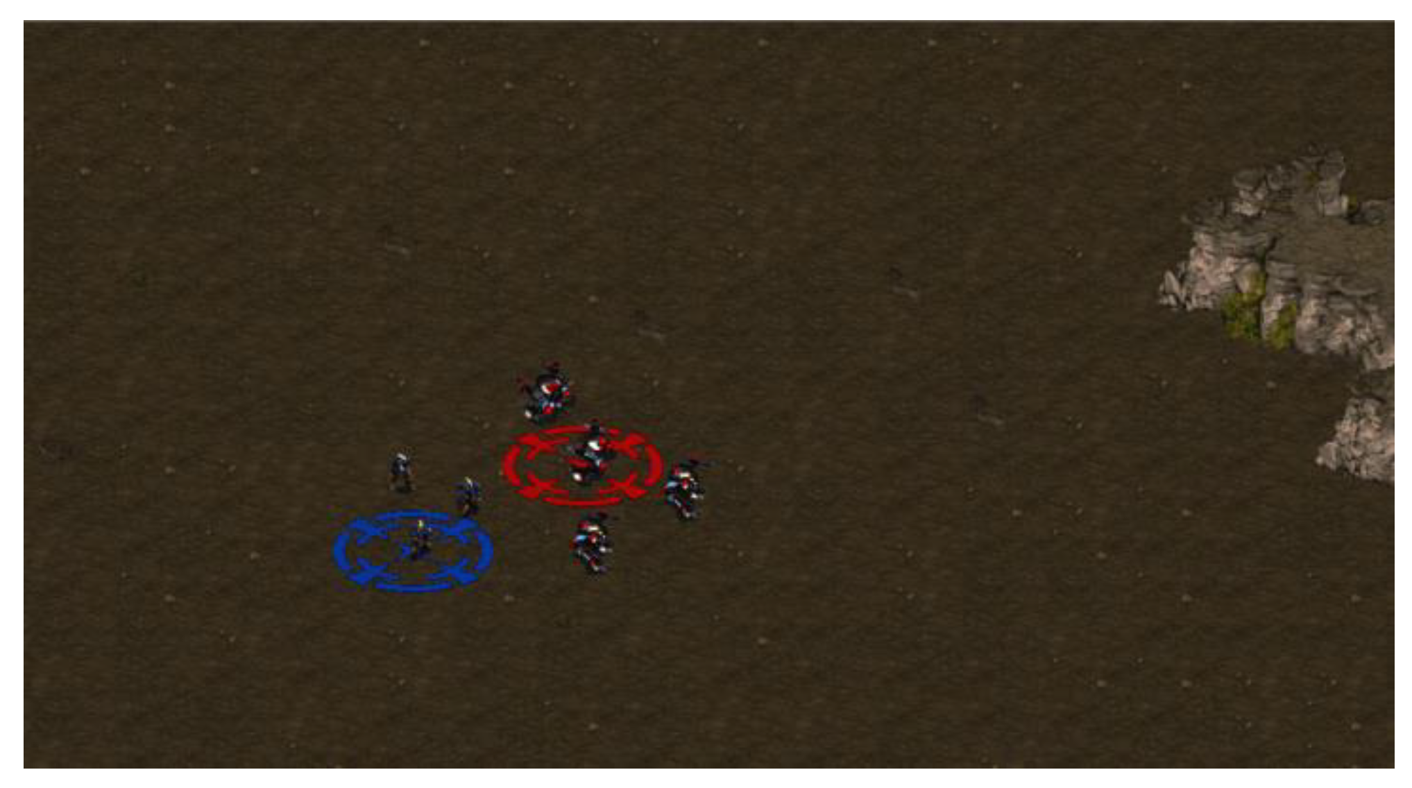
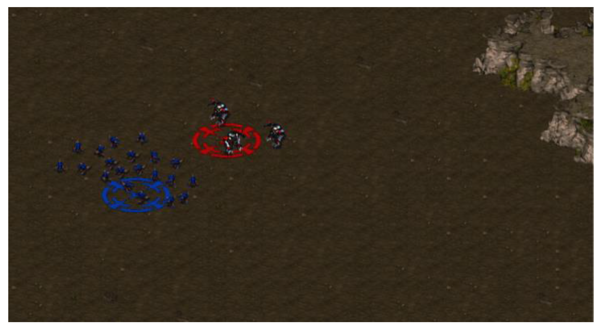
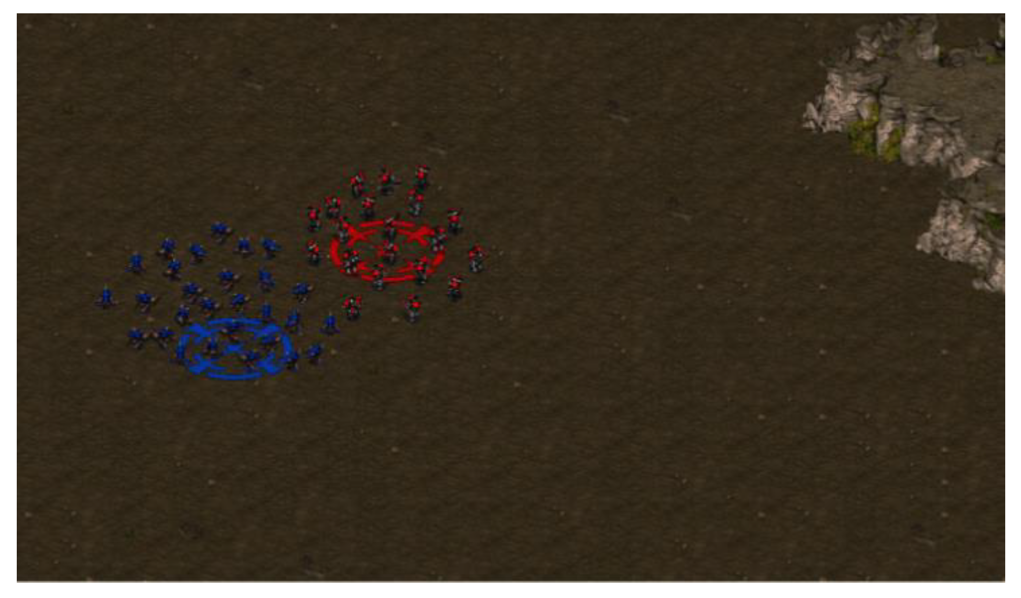
8. Experiment on Tank War Task
8.1. Experimental Configuration for Tank War Task
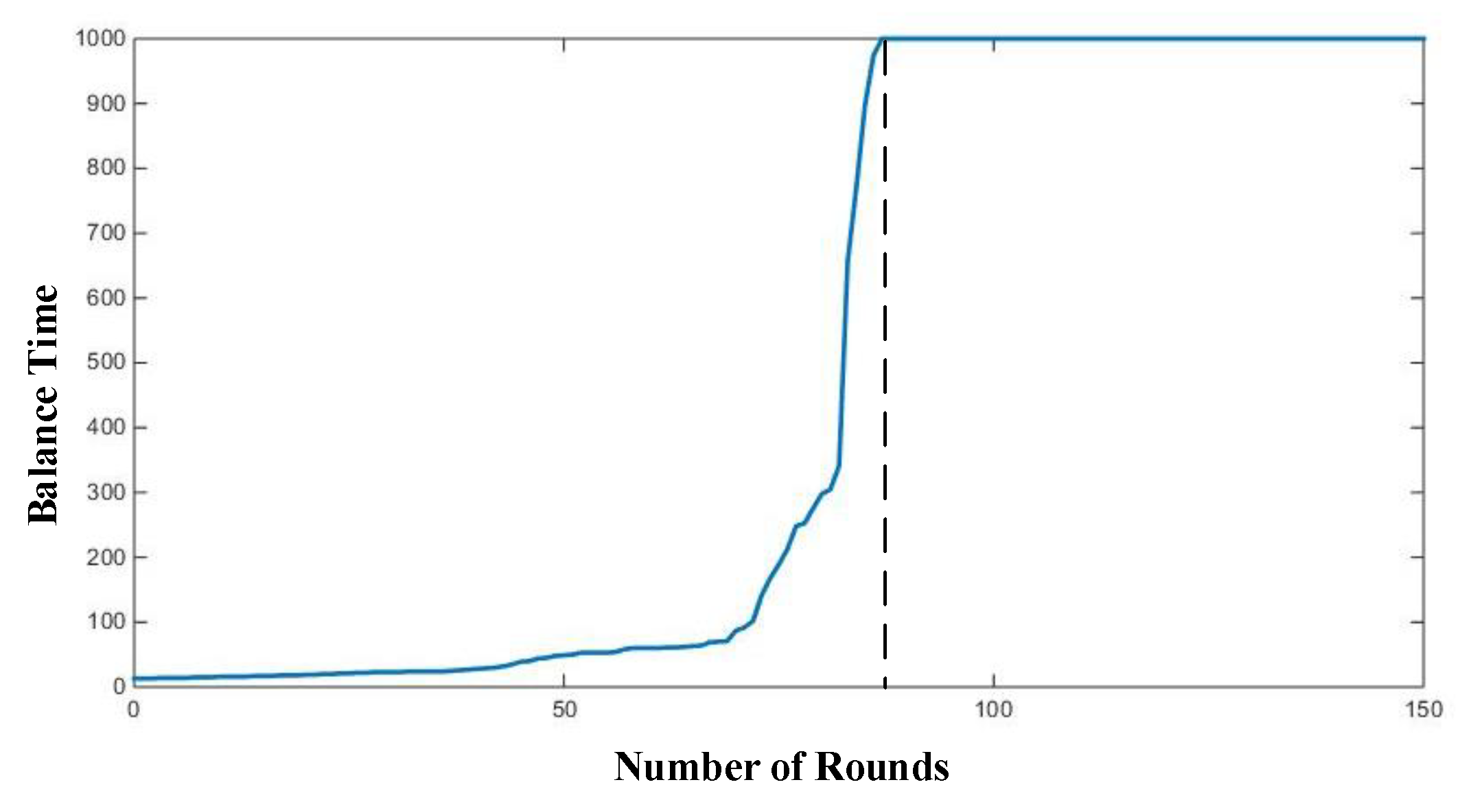
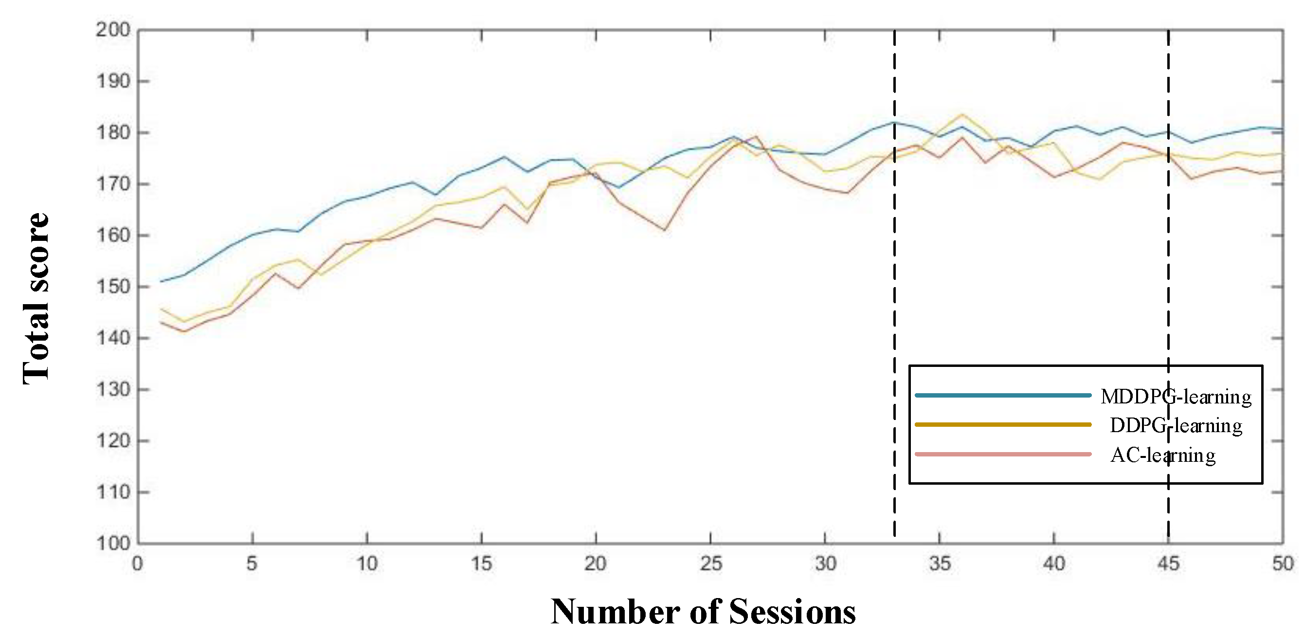
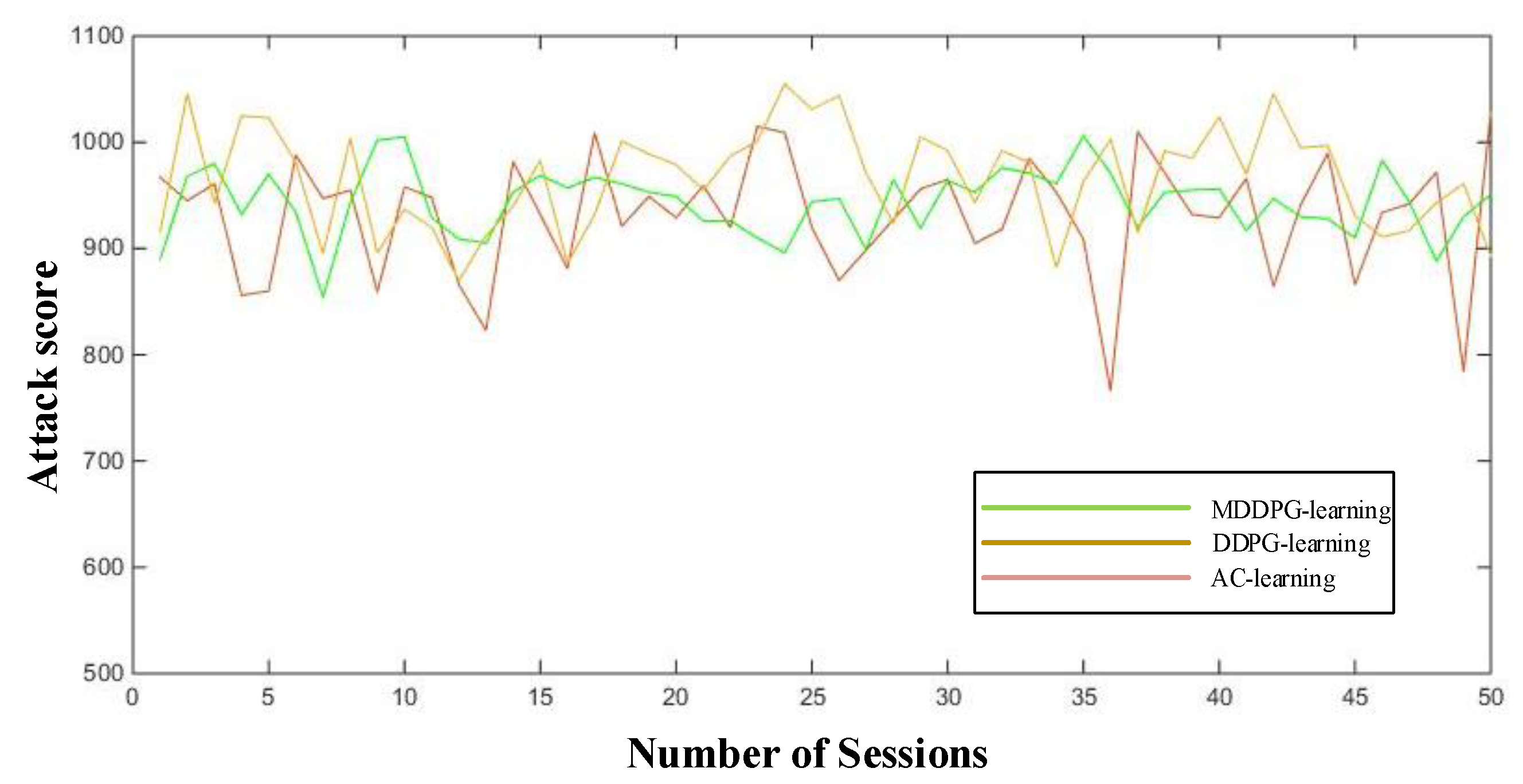
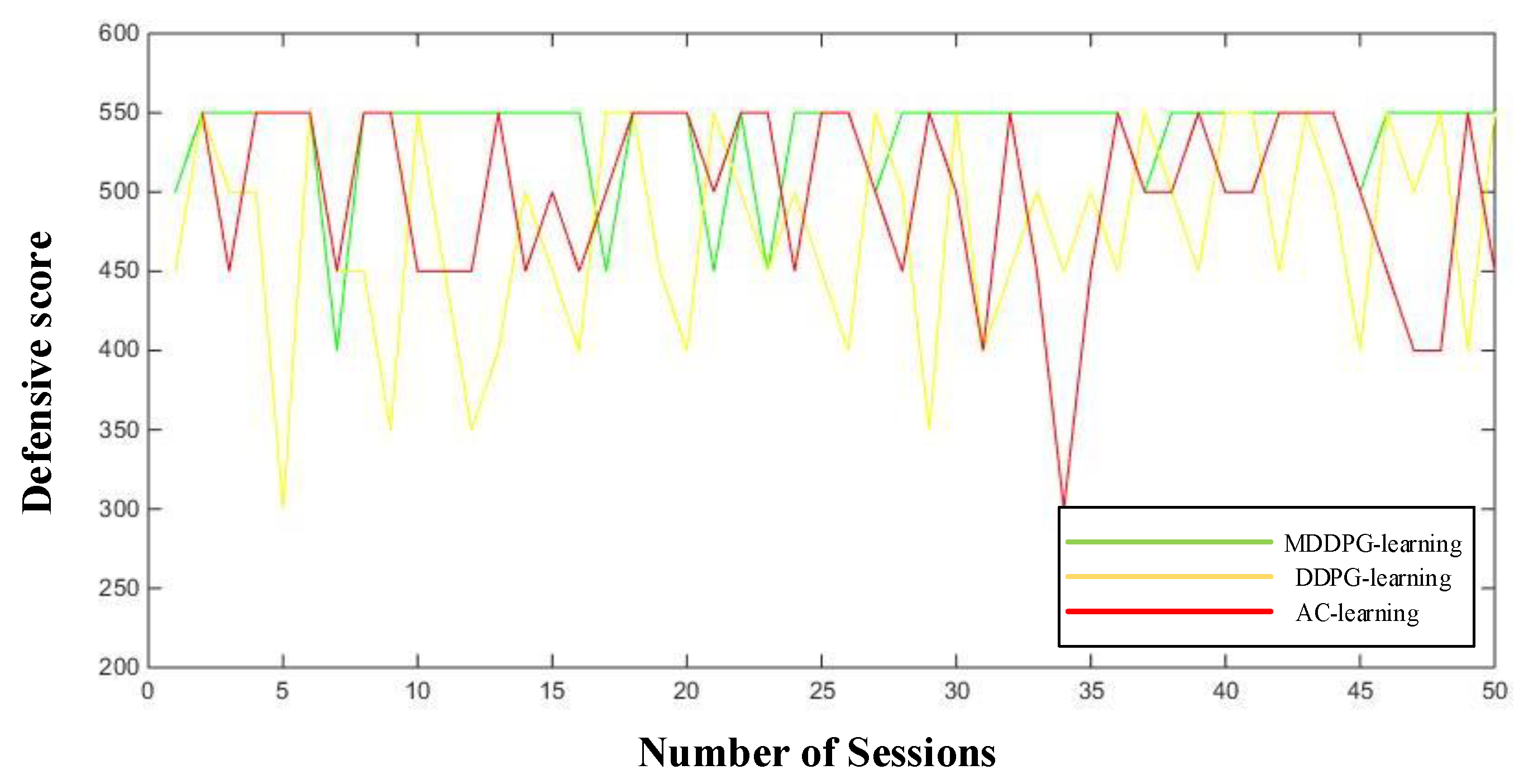
8.2. Experimental Results and Analysis
9. Conclusions
Author Contributions
Funding
Conflicts of Interest
References
- Emary, E.; Hossam; Zawbaa, M.; Grosan, C. Experienced Gray Wolf Optimization Through Reinforcement Learning and Neural Networks. IEEE Trans. Neural Netw. Learn. Syst. 2018, 29, 681–694. [Google Scholar] [CrossRef]
- Kiumarsi, B.; Kyriakos; Vamvoudakis, G.; Modares, H.; Lewis, F.L. Optimal and Autonomous Control Using Reinforcement Learning: A Survey. IEEE Trans. Neural Netw. Learn. Syst. 2018, 29, 2042–2062. [Google Scholar] [CrossRef]
- Pradeep, D.J.; Noel, M.M.; Arun, N. Nonlinear control of a boost converter using a robust regression based reinforcement learning algorithm. Eng. Appl. Artif. Intell. 2016, 52, 1–9. [Google Scholar] [CrossRef]
- Hu, C.; Xu, M. Adaptive Exploration Strategy With Multi-Attribute Decision-Making for Reinforcement Learning. IEEE Access 2020, 8, 32353–32364. [Google Scholar] [CrossRef]
- Tan, X.; Chng, C.B.; Su, Y.; Lim, K.B.; Chui, C.K. Robot-assisted training in laparoscopy using deep reinforcement learning. IEEE Robot. Autom. Lett. 2019, 4, 485–492. [Google Scholar] [CrossRef]
- Li, Z.; Liu, J.; Huang, Z.; Peng, Y.; Pu, H.; Ding, L. Adaptive impedance control of human–robot cooperation using reinforcement learning. IEEE Trans. Ind. Electron. 2017, 64, 8013–8022. [Google Scholar] [CrossRef]
- Yuan, Y.; Li, Z.; Zhao, T.; Gan, D. DMP-based Motion Generation for a Walking Exoskeleton Robot Using Reinforcement Learning. IEEE Trans. Ind. Electron. 2019, 67, 3830–3839. [Google Scholar] [CrossRef]
- Balducci, F.; Grana, C.; Cucchiara, R. Affective level design for a role-playing videogame evaluated by a brain-computer interface and machine learning methods. Vis. Comput. 2016, 33, 1–15. [Google Scholar] [CrossRef]
- Hu, C.; Xu, M. Fuzzy Reinforcement Learning and Curriculum Transfer Learning for Micromanagement in Multi-Robot Confrontation. Information 2019, 10, 341. [Google Scholar] [CrossRef]
- Othman, N.; Decraene, J.; Cai, W.; Hu, N.; Gouaillard, A. Simulation-based optimization of StarCraft tactical AI through evolutionary computation. J. Yunnan Agric. Univ. 2012, 3, 639–643. [Google Scholar]
- Ontanon, S.; Synnaeve, G.; Uriarte, A.; Richoux, F. A Survey of Real-Time Strategy Game AI Research and Competition in StarCraft. IEEE Trans. Comput. Intell. AI Games 2013, 5, 293–311. [Google Scholar] [CrossRef]
- Shantia, A.; Begue, E.; Wiering, M. Connectionist reinforcement learning for intelligent unit micro management in StarCraft. In Proceedings of the International Joint Conference on Neural Networks, San Jose, CA, USA, 31 July–5 August 2011; pp. 1794–1801. [Google Scholar]
- Wender, S.; Watson, I. Applying reinforcement learning to small scale combat in the real-time strategy game StarCraft: Broodwar. In Proceedings of the IEEE Conference on Computational Intelligence and Games, Granada, Spain, 11–14 September 2012; pp. 402–408. [Google Scholar]
- Mansoor, A.; Juan; Cerrolaza, J.; Idrees, R.; Biggs, E.; Alsharid, M.A.; Avery, R.A.; Linguraru, M.G. Deep Learning Guided Partitioned Shape Model for Anterior Visual Pathway Segmentation. IEEE Trans. Med Imaging 2016, 35, 1856–1865. [Google Scholar] [CrossRef] [PubMed]
- Liu, Y.; Tang, L.; Tong, S.; Chen, C.L.; Li, D.J. Reinforcement Learning Design-Based Adaptive Tracking Control With Less Learning Parameters for Nonlinear Discrete-Time MIMO Systems. IEEE Trans. Neural Netw. Learn. Syst. 2015, 26, 165–176. [Google Scholar] [CrossRef] [PubMed]
- Xu, J.; Hou, Z.; Wang, W.; Xu, B.; Zhang, K.; Chen, K. Feedback deep deterministic policy gradient with fuzzy reward for robotic multiple peg-in-hole assembly tasks. IEEE Trans. Ind. Inform. 2018, 15, 1658–1667. [Google Scholar] [CrossRef]
- Machado, M.C.; Bellemare, M.G.; Bowling, M. A laplacian framework for option discovery in reinforcement learning. In Proceedings of the 34th International Conference on Machine Learning-Volume 70. JMLR. org, Sydney, Australia, 6–11 August 2017; pp. 2295–2304. [Google Scholar]
- Jialin, P.S.; Qiang, Y. A Survey on Transfer Learning. IEEE Trans. Knowl. Data Eng. 2010, 22, 1345–1359. [Google Scholar]
- Wei, Q.; Lewis, F.L.; Sun, Q.; Yan, P.; Song, R. Discrete-time deterministic Q-learning: A novel convergence analysis. IEEE Trans. Cybern. 2016, 47, 1224–1237. [Google Scholar] [CrossRef]
- Luo, B.; Liu, D.; Huang, T.; Wang, D. Model-free optimal tracking control via critic-only Q-learning. IEEE Trans. Neural Netw. Learn. Syst. 2016, 27, 2134–2144. [Google Scholar] [CrossRef]
- Vamvoudakis, K.G.; Lewis, F.L. Online actor–critic algorithm to solve the continuous-time infinite horizon optimal control problem. Automatica 2010, 46, 878–888. [Google Scholar] [CrossRef]
- Zhang, Z.; Wang, R.; Yu, F.R.; Fu, F.; Yan, Q. QoS Aware Transcoding for Live Streaming in Edge-Clouds Aided HetNets: An Enhanced Actor-Critic Approach. IEEE Trans. Veh. Technol. 2019, 68, 11295–11308. [Google Scholar] [CrossRef]
- Wang, Z.; Dedo, M.I.; Guo, K.; Zhou, K.; Shen, F.; Sun, Y.; Guo, Z. Efficient recognition of the propagated orbital angular momentum modes in turbulences with the convolutional neural network. IEEE Photonics J. 2019, 11, 1–14. [Google Scholar] [CrossRef]
- Schurz, H. Preservation of probabilistic laws through Euler methods for Ornstein-Uhlenbeck process. Stoch. Anal. Appl. 1999, 17, 463–486. [Google Scholar] [CrossRef]
- Shao, K.; Zhu, Y.; Zhao, D. Starcraft micromanagement with reinforcement learning and curriculum transfer learning. IEEE Trans. Emerg. Top. Comput. Intell. 2018, 3, 73–84. [Google Scholar] [CrossRef]
- Garten, F.; Vrijmoeth, J.; Schlatmann, A.R.; Gill, R.E.; Klapwijk, T.M.; Hadziioannou, G. Light-emitting diodes based on polythiophene: Influence of the metal work function on rectification properties. Synth. Met. 1996, 76, 85–89. [Google Scholar] [CrossRef]
- Miao, Y.; Li, J.; Wang, Y.; Zhang, S.; Gong, Y. Simplifying long short-term memory acoustic models for fast training and decoding. In Proceedings of the 2016 IEEE International Conference on Acoustics, Speech and Signal Processing (ICASSP), Shanghai, China, 20–25 March 2016; pp. 2284–2288. [Google Scholar]
- Wang, H.; Gao, Y.; Chen, X.G. Transfer of Reinforcement Learning: The State of the Art. Acta Electron. Sin. 2008, 36, 39–43. [Google Scholar]
- Lillicrap, T.P.; Hunt, J.J.; Pritzel, A.; Heess, N.M.; Erez, T.; Tassa, Y.; Silver, D.; Wierstra, D. Continuous control with deep reinforcement learning. In Proceedings of the International Conference on Learning Representations, San Diego, CA, USA, 7–9 May 2015. abs/1509.02971. [Google Scholar]
- Nair, A.; McGrew, B.; Andrychowicz, M.; Zaremba, W.; Abbeel, P. Overcoming exploration in reinforcement learning with demonstrations. In Proceedings of the 2018 IEEE International Conference on Robotics and Automation (ICRA), Brisbane, Australia, 21–26 May 2018; pp. 6292–6299. [Google Scholar]
- De Hauwere, Y.; Devlin, S.; Kudenko, D.; Nowé, A. Context-sensitive reward shaping for sparse interaction multi-agent systems. Knowl. Eng. Rev. 2016, 31, 59–76. [Google Scholar] [CrossRef]
- Kompella, V.R.; Stollenga, M.; Luciw, M.; Schmidhuber, J. Continual curiosity-driven skill acquisition from high-dimensional video inputs for humanoid robots. Artif. Intell. 2017, 247, 313–333. [Google Scholar] [CrossRef]
- Mikhail, F.; Jürgen, L.; Marijn, S.; Alexander, F.; Jürgen, S. Curiosity driven reinforcement learning for motion planning on humanoids. Front. Neurorobotics 2014, 7, 1–15. [Google Scholar]


| Parameter | Value |
|---|---|
| Learning rate of DRL | 0.0015 |
| Discount rate | 0.95 |
| Mini-batch size | 64 |
| Soft target update | 0.001 |
| Maximum time steps | 1000 |
| Adam algorithm factors and | 0.9 |
| Intermediate Task 1 | Intermediate Task 2 | Intermediate Task 3 | |
|---|---|---|---|
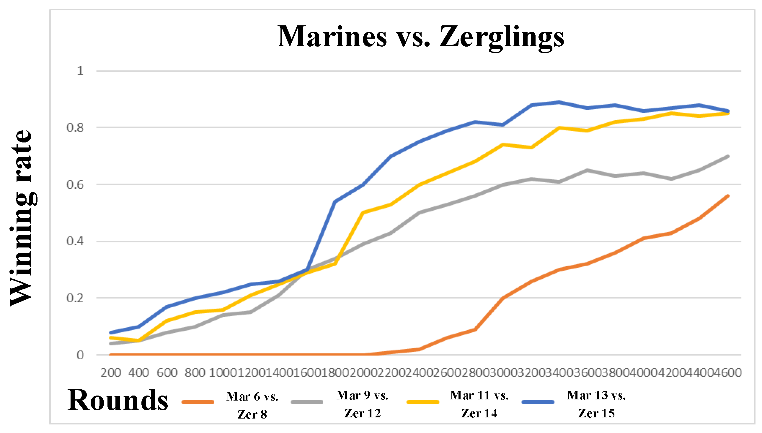
| Mar13 vs. Zer15 | Mar 6 vs. Zer 8 | Mar 9 vs. Zer 12 | Mar 11 vs. Zer 14 |
| Mar 23 vs. Zer 35 | Mar 14 vs. Zer 16 | Mar 18 vs. Zer 25 | Mar 22 vs. Zer 29 |
| Parameter | Value |
|---|---|
| Learning rate of DRL | 0.001 |
| Discount rate | 0.8 |
| Mini-batch size | 32 |
| Soft target update | 0.01 |
| Maximum HPs | 100 |
| Adam algorithm factor and | 0.9 |
© 2020 by the author. Licensee MDPI, Basel, Switzerland. This article is an open access article distributed under the terms and conditions of the Creative Commons Attribution (CC BY) license (http://creativecommons.org/licenses/by/4.0/).
Share and Cite
Hu, C. A Confrontation Decision-Making Method with Deep Reinforcement Learning and Knowledge Transfer for Multi-Agent System. Symmetry 2020, 12, 631. https://doi.org/10.3390/sym12040631
Hu C. A Confrontation Decision-Making Method with Deep Reinforcement Learning and Knowledge Transfer for Multi-Agent System. Symmetry. 2020; 12(4):631. https://doi.org/10.3390/sym12040631
Chicago/Turabian StyleHu, Chunyang. 2020. "A Confrontation Decision-Making Method with Deep Reinforcement Learning and Knowledge Transfer for Multi-Agent System" Symmetry 12, no. 4: 631. https://doi.org/10.3390/sym12040631
APA StyleHu, C. (2020). A Confrontation Decision-Making Method with Deep Reinforcement Learning and Knowledge Transfer for Multi-Agent System. Symmetry, 12(4), 631. https://doi.org/10.3390/sym12040631