Abstract
Considering the characteristics such as fuzziness and greyness in real decision-making, the interval grey triangular fuzzy number is easy to express fuzzy and grey information simultaneously. And the partition Bonferroni mean (PBM) operator has the ability to calculate the interrelationship among the attributes. In this study, we combine the PBM operator into the interval grey triangular fuzzy numbers to increase the applicable scope of PBM operators. First of all, we introduced the definition, properties, expectation, and distance of the interval grey triangular fuzzy numbers, and then we proposed the interval grey triangular fuzzy numbers partitioned Bonferroni mean (IGTFPBM) and the interval grey triangular fuzzy numbers weighted partitioned Bonferroni mean (IGTFWPBM), the adjusting of parameters in the operator can bring symmetry effect to the evaluation results. After that, a novel method based on IGTFWPBM is developed for solving the grey fuzzy multiple attribute group decision-making (GFMAGDM) problems. Finally, we give an example to expound the practicability and superiority of this method.
1. Introduction
Multiple attribute group decision-making (MAGDM) is the process of comparing and choosing the best alternative by analyzing the evaluations of multiple attributes aggregated from decision-makers. And MAGDM problems have a wide application in real life, such as effect evaluation of environmental protection policies formulated by the government [1], the evaluation of international cooperation plans for energy development [2], the assessment of the comprehensive strength of different schools [3], the comparison of various schemes by enterprises in business negotiations [4], and the selection of enterprises’ purchasing schemes [5]. Most of the MAGDM problems exist fuzziness and uncertainty, which is because people’s ideology is subjective and complex. Besides, decision-makers may fall into the predicament of the lack of information when evaluating alternatives, which shows the characteristics of grey decision making. In practical decision making, fuzziness and greyness are often existing at the same time, which is called the grey fuzzy multiple attribute group decision-making (GFMAGDM) problem.
To solve GFMGADM problems completely and improve the accuracy of decision results, more and more research has been carried out and expanded from the expression forms of grey information and fuzzy information [6], the integrated calculation method of grey information and fuzzy information [7], the construction of decision system based on grey fuzzy information [8], and the application problems based on grey fuzzy information [9,10]. Bu and Zhang [11] interpreted the grey degree as a level of uncertainty of information, converted the grey numbers into the three-parameter interval numbers, and gave an approach of interval numbers to sort all alternatives. However, they did not give a definite formula when comparing any two alternatives. Based on the literature [11], Luo and Liu [12] used the optimization theory and the maximum entropy criterion to give the method about GFMGADM problems under the conditions that the attributes’ weights are known or unknown. Jin and Lou [13,14] considered the fuzziness and greyness in the decision-making process, calculated the distinctions between positive and negative ideal solutions of all alternatives and used satisfaction as weights to adjust the attributes’ ranking order. The above researches mainly introduced a method about the grey part of grey fuzzy numbers, which can pragmatically handle the problem of lacking information. However, the fuzzy part shown as exact numbers is difficult to represent the complexity of objective things and fuzziness of people’s thinking. Zhu et al. [15] tried to express the fuzzy part with interval numbers and combine with the grey part to express grey fuzzy numbers. Jin and Liu [16] proposed the interval grey linguistic variables, the fuzzy part was represented by interval grey linguistic variables and introduced an approach to undertake GFMADM problems. Interval grey trapezoid fuzzy linguistic variables proposed by Yin et al. [17] can use more information to improve the accuracy of evaluation. Wang and Wang [18] proposed grey linguistic 2-tuple terms to express the priority option of a decision-maker in a grey fuzzy environment. The above expressions used to solve GFMADM problems to reflect fuzzy information and grey information are relatively simple, especially in the fuzzy part, the fuzzy information is expressed by interval numbers and linguistic variables. Although the calculation process has the advantage of simplicity and rapidity, the calculation results are often rough and difficult to be applied to accurate evaluation problems in the military field and medical field.
In recent years, there are extensive researches on decision methods and operators in a grey fuzzy environment. Jin and Liu [16] constructed the TOPSIS (Technique for Order Preference by Similarity to an Ideal Solution) method based on interval grey linguistic variables to solve the decision-making problem in a grey fuzzy environment. Wang et al. [19] extended the traditional SIR ( Superiority and Inferiority Ranking) model to interval grey linguistic variables and proposed the SIR Choquet method considering the independence of multi-attribute variables. Liu and Zhang [20] proposed the interval grey linguistic variables weighted geometric aggregation (IGLWGA) operator, the interval grey linguistic variables ordered weighted geometric aggregation (IGLOWGA) operator, and the interval grey linguistic variable hybrid weighted geometric aggregation (IGLHWGA) operator, and developed a new method referred to IGLHWGA operators. Liu [21] proposed the interval grey linguistic variables weighted aggregation (IGLWA) operator and the interval grey linguistic variables weighted aggregation (IGLHWA) operator and applied them to a method of sorting the alternatives. Liu et al. [22] proposed the interval grey uncertain linguistic generalized ordered weighted averaging (IGULGOWA) operator and the interval grey uncertain linguistic generalized hybrid averaging (IGULGHA) operator to solve GFMADM problems according to interval grey uncertain linguistic information. The above methods and operators do not consider the interrelationship among attribute variables. However, in the process of evaluation, there may be some correlation among the attribute variables. Back in 1950, Bonferroni [23] proposed the Bonferroni mean (BM), which were to be judged alternatives by establishing conjunction between each attribute variable. Yager [24,25,26] deepened the understanding of the Bonferroni mean in 2009, firstly it was proposed that BM could be used to calculate the interrelationship among any pair of attributes and suggested replace the simple weighted operator with other more complex operators. At present, BM has been widely used in different fuzzy information and different environments due to its ability to determine the optimal alternative according to interrelationship [27,28,29,30,31,32]. Tian et al. [33] proposed the grey linguistic weighted Bonferroni mean operator to solve GFMADM problems which exit interrelationship between each attribute. However, BM assumes that there exists an interrelationship between any two attributes, and it is difficult to match the actual decision process. Focusing on this problem, Dutta and Guha [29] proposed the partitioned Bonferroni mean (PBM) which is based on the premise that all attributes are divided into some classes based on the interrelationship of each attribute variable in the actual decision, any attribute variable in each class is required to be only related to attribute variables in the same class and be not related to attribute variables in other classes. For example, when choosing the mobile phone, we may evaluate mobile phones from the following four aspects: appearance design (), the inner performance (), brand influence (), and after-sales service (). The four attributes can be divided into two classes: and . It is not difficult to find that is unrelated to , and there is no interrelationship between and . After that, more and more scholars have perfected PBM operators. The intuitionistic uncertain linguistic partitioned Bonferroni mean (IULPBM) operator [34] and the intuitionistic fuzzy interaction partitioned Bonferroni mean (IFWIPBM) operator [35] are proposed to calculate the internal correlation of attribute variables in an intuitionistic fuzzy environment. Yin et al. [36] developed the trapezoidal fuzzy two-dimensional linguistic partitioned Bonferroni mean (TF2DLPBM) operator for solving MAGDM problems. Liu and Liu [37] proposed the PBM operator for two-dimensional uncertain linguistic variables (2DULVs) and developed a new method.
In the actual decision-making process, different decision-makers have different cognition of the alternatives, and the same decision-maker has different cognition degrees of different attributes of the same alternative. Therefore, the comparability of the evaluation results of different decision-makers is weak, and the reliability of the comprehensive results is insufficient. At present, the existing fuzzy variables are mostly used for the decision-makers subjective evaluation information of the evaluation program, and there are few pieces of research on the objective cognition degree in the evaluation process. In this paper, we proposed the interval grey triangular fuzzy numbers which fuzzy part in the form of triangular fuzzy numbers and the grey part expressed by interval numbers. The fuzzy part of the interval grey triangular fuzzy numbers is used to express the subjective evaluation of decision-makers on the attribute variables of alternatives, and the grey part is used to indicate the objective cognition degree of the decision-maker to the attribute variables of the alternatives. The increase of the grey part is a supplement to the reliability of the original fuzzy evaluation. When the value of the grey part is smaller, it means that the decision-maker knows more about the alternatives and his evaluation result is more convincing, in other words, the reliability of the fuzzy part is higher. Compared with the existing form of expression of uncertain information, the interval grey triangular fuzzy numbers can reflect decision-makers’ subjective evaluation and objective cognition of evaluation objects, the decision-making information is more comprehensive. At the same time, the interval grey triangular fuzzy numbers can transform with interval grey linguistic variables, interval grey interval number and other grey fuzzy forms, which has a wide scope of application.
Until now, in the grey fuzzy environment, there is no method considering the internal structure and interrelationship among the attributes. And then, we extend the PBM operator to the interval grey triangular fuzzy numbers, partitioned all attributes into several classes and ensured that any attribute is only interrelated to other attributes in the same class, after all these, we proposed the interval grey triangular fuzzy numbers partitioned Bonferroni mean (IGTFPBM) and the interval grey triangular fuzzy numbers weighted partitioned Bonferroni mean (IGTFWPBM). Based on the IGTFWPBM operators, we introduced an approach for solving GFMAGDM problems. The method proposed in this paper can consider the interrelationship among attributes, classify and integrate the calculation of attributes, which is more consistent with the decision logic of practical problems. The parameters p and q in the operator can reflect the decision maker’s attitude towards the hierarchical relationship of attributes, and the decision-maker can obtain different decision ordering by adjusting the parameter size. In addition, symmetric adjustment of parameters p and q will produce a symmetry effect on the expectation of the alternative.
The remainder of this paper is organized as follows. We introduce some conception of the triangular fuzzy number, grey math, and PBM briefly in Section 2. Section 3 gives the definition, calculation rules, distances, and comparative methods of the interval grey triangular fuzzy numbers. We proposed the IGTFPBM operators and IGTFWPBM operators by considering the interrelationship in the fuzzy and grey information in Section 4. In Section 5, we developed an approach for undertaking the GFMAGDM problems based on IGTFWPBM. In Section 6, we gave an instance to explain the new method. Finally, we discussed the conclusion in Section 7.
2. Preliminaries
In this section, we recalled the form of the triangular fuzzy numbers and grey math briefly, and we reviewed the concepts of BM and the PBM, which are foundations of the decision-making methods we proposed.
2.1. The Triangular Fuzzy Number
Definition 1.
[38,39] A triangular fuzzy numberis defined as, which satisfies the condition, and the calculation rules of membership function are shown as follows:
when , the triangular fuzzy number can be transformed into a crisp number.
2.2. Grey Fuzzy Math
Definition 2.
[16,40] Let be grey fuzzy set in space X.is the fuzzy subset in the space X = {x} andis the grey subset in the space X = {x}. The membership degreeofis the fuzzy number in the interval [0, 1], and the grey degreeof is the grey number in the interval [0, 1].
And the simplified form is:
where is called the fuzzy part of , and is called the grey part of .
2.3. Partitioned Bonferroni Mean
Definition 3.
[23] For any, the BM operator as follows:
where is the set of a non-negative real number, p and q are the parameters of decision-makers. BM operators can calculate the interrelationship between any attributes. However, the operator is limited by the assumption that there is an interrelationship among each attribute, so some independent attributes cannot be included in the calculation. Under the circumstances, Dutta and Guha [31] proposed PBM.
Definition 4.
[29] For any, the PBM operator as follows:
where is the set of a non-negative real number, e is the number of classes and is number of attributes in the same class.
3. Interval Grey Triangular Fuzzy Numbers
In this section, we built the interval grey triangular fuzzy numbers. After that, we gave the definition, operation rules, distance, and comparing methods of the interval grey triangular fuzzy numbers.
3.1. The Definition of Interval Grey Triangular Fuzzy Numbers
Definition 6.
Let be any grey fuzzy number, if the fuzzy part is a triangular fuzzy number, and its grey partis closed intervalin the interval [0, 1], then is called an interval grey triangular fuzzy number.
It is worth emphasizing that the fuzzy part (triangular fuzzy number) and grey part (the interval grey number) are mutually independent. In the traditional sense, both fuzzy information and grey information can express uncertain information. Fuzzy information represents the subjective evaluation of the decision-maker on the alternatives, while grey information represents the incomplete cognition of decision-makers to the objective existence of certain characteristics of alternatives [41]. The fuzzy part of the interval grey triangular fuzzy numbers expresses the subjective evaluation of the decision-maker on the attributes of the alternatives, and the grey part indicates the objective cognition degree of the decision-maker to the attributes of alternatives, which is to evaluate the alternatives from two different dimensions. Therefore, the fuzzy part (triangular fuzzy number) and grey part (the interval grey number) are mutually independent, and the form used to express grey information and fuzzy information is also consistent with some research results [16,20,21,22].
3.2. The Operation Rules of the Interval Grey Triangular Fuzzy Numbers
Let and be any two-interval grey triangular fuzzy numbers. The operation rules of interval grey triangular fuzzy numbers are defined as bellows:
Supposed that , and be the three interval grey triangular fuzzy numbers. The interval grey triangular fuzzy numbers satisfied the following properties.
3.3. The Distance between the Two-Interval Grey Triangular Fuzzy Numbers
Definition 7.
Letandbe any two-interval grey triangular fuzzy numbers. Y is the set of the interval grey triangular fuzzy numbers,be the mapping,. If, and satisfied the following formula:
- (1)
- ,
- (2)
- ;
- (3)
Thenis called the distance between the interval grey triangular fuzzy numbers.
Definition 8.
Letand be any two-interval grey triangular fuzzy numbers variables, then the distance between and is defined as follows:
The distance measure between the interval grey triangular fuzzy numbers satisfies the following properties:
(1) Let and be the two-interval grey triangular fuzzy numbers. When tend to 0, close to , when , .
(2) Let , and be the three interval grey triangular fuzzy numbers. The necessary and sufficient condition for to be closer to than is that . If , the distance between and is equal to the distance between and .
3.4. The Comparing Method of Interval Grey Triangular Fuzzy Numbers
Definition 9.
Let be an interval grey triangular fuzzy numbers variable, then the expectation of interval grey triangular fuzzy numbers is defined as below:
Let and be any two-interval grey triangular fuzzy numbers variables, We can decide by comparing the expected size of and , if , then , or vice versa.
The comparison method of a grey part was proposed by Jin and Liu [16], the comparison method of fuzzy part reference interval number [42], and the solution process of the comparison method of triangular fuzzy number is as follows:
Let be the triangular fuzzy number, then the cut set of is defined as ,, is closed interval , then , and .
Let be the triangular fuzzy number, then:
Then is called the fuzzy OWA (F-OWA) operator.
Specially, when (r > 0), then:
Aggregate the fuzzy part of by F-OWA operator, transform the triangular fuzzy number into real numbers that calculating the value of .
4. The Interval Grey Triangular Fuzzy Numbers Partitioned Bonferroni Mean Operators and Interval Grey Triangular Fuzzy Numbers Weighted Partitioned Bonferroni Mean Operators
In this section, we applied the PBM into the fuzzy and grey information and proposed the IGTFPBM and IGTFWPBM operators.
4.1. The Interval Grey Triangular Fuzzy Numbers Partitioned Bonferroni Mean Operators
Definition 10.
Let () be a group of interval grey triangular fuzzy numbers. For any, the IGTFPBM:, if
where is the set of all interval grey triangular fuzzy numbers variables anddenotes the cardinality of.
Theorem 1.
Let () be a collection of the interval grey triangular fuzzy number, then the result aggregated by IGTFPBM operators is still an interval grey triangular fuzzy numbers variable, and also
Proof.
Because of the operational rules of the interval grey triangular fuzzy numbers variables, we have:
and:
Then:
and:
which completes the proof. □
Theorem 2.
(Idempotency): Let,,, and all() is equal, i.e.,,then,
Proof.
Since , then:
which completes the proof. □
Theorem 3.
(Commutativity) Letbe any permutation of, then:
Proof.
Since is any permutation of , then:
which completes the proof. □
Theorem 4.
(Monotonicity) If (), then:
Proof.
□
Theorem 5.
(Symmetry) Let,() be a collection of the interval grey triangular fuzzy number, then
Proof.
when e = 1 and , then, the IGTFPBM operators reduce to interval grey triangular fuzzy numbers Bonferroni mean (IGTFBM).
We gave some special cases of the IGTFPBM operators as follows:
Case 1. If q = 0, then, Equations (23) and (24) are transformed as follows:
Case 2. If p = 1 and q = 0, then, Equations (23) and (24) are transformed as follows:
Case 3. If p = 2 and q = 0, then, Equations (23) and (24) are transformed as follows:
Case 4. If p = 1 and q = 1, then, Equations (23) and (24) are transformed as follows:
□
4.2. The Interval Grey Triangular Fuzzy Numbers Weighted Partitioned Bonferroni Mean Operator
IGTFPBM can capture the interrelationship, that operator assumes that the attributes are equally important, however, this is not in line with fact. Therefore, we establish the IGTFWPBM considering the different attributes have different importance and then, we gave the related properties of new operators.
Definition 11.
Let () be a group of the interval grey triangular fuzzy numbers variables. For any, the IGTFWPBM:, if
where is the set of all interval grey triangular fuzzy numbers, and represents the importance of each attribute variable and satisfies the conditions: , . Then WIGTFPBM called WIGTFPBM aggregation operator.
Theorem 5.
Let () be a collection of the interval grey triangular fuzzy numbers variables, andis the weight vector of(),,, then, the result is still an interval grey triangular fuzzy numbers variable, and also:
The proof of this theorem is similar to that of Theorem 1, so we left it out here.
Theorem 6.
(Commutativity) Letbe any permutation of, then
The proof was omitted here, please refer to the proof of Theorem 3.
Theorem 7.
(Monotonicity) If (), then:
The proof is omitted here, please refer to the proof of Theorem 4.
Theorem 8.
(Symmetry) Let,() be a collection of the interval grey triangular fuzzy number, then:
The proof is omitted here, please refer to the proof of Theorem 5.
In particular, the IGTFPBM operator is one special case of IGTFWPBM operator, the conversion relationship between IGTFPBM operator and IGTFWPBM operator is shown as follows:
And then, we discussed some special cases of IGTFWPBM as follows:
Case 1. If q = 0, then, Equation (34) and Equation (35) are transformed as follows:
Case 2. If p = 1 and q = 0, then, Equations (34) and (35) are transformed as follows:
Case 3. If p = 2 and q = 0, then, Equations (34) and (35) are transformed as follows:
Case 4. If p = 1 and q = 1, then, Equations (34) and (35) are transformed as follows:
5. A GFMAGDM Method Based on IGTFWPBM
In this section, we introduced a method to solve the GFMAGDM problems in the context of grey and fuzzy information. In real decision-making, the group of decision-makers needs to evaluate the optimal decision from the set of m alternatives based on the n attributes . Because some attributes may be interrelated with other attributes, we divided n attributes into e classes , and ensured that each attribute is only interrelated with other attributes in the same class. The weights of the attributes can be expressed by ,, . The weights of the decision-makers can be expressed by , and . Suppose that is the decision matrix where () represents the structure of the interval grey triangular fuzzy numbers, which expresses that the decision maker evaluate the attribute of the attribute. We collected the above information about each alternative and ranked the order of alternatives. And the specific steps are as follows:
Step 1.
Normalizing the interval grey triangular fuzzy numbers.
In general, attributes have directionality, and we changed some attributes’ direction to ensure that benefit attributes and cost attributes have the same direction. Meanwhile, we should normalize the attributes because of the differences in evaluation standards from different decision-makers.
Suppose is the normalized matrix of decision matrix where , and the normalization method is as follows:
- (1)
- For benefit attributes:where .
- (2)
- For cost attributes:where .
Step 2.
Aggregating the information from decision-makers.
Suppose is the group decision matrix by aggregating from normalized matrix by weighting method. Where , as follows:
Step 3.
Calculating the comprehensive evaluation value.
Calculating each alternative’s evaluation value by IGTFWPBM operators. Where as follows:
Step 4.
Calculating the expectation for the alternative’s IGTFWPBM operator.
Step 5.
Ranking the alternatives.
Ranking the alternatives based on the expectation value and selecting the best alternative.
6. Illustrative Examples
In this section, we gave an example to explain the application of IGTFWPBM operators in solving GFMGADM problems in Section 6.1. In Section 6.2, the variation of parameters on the evaluation results and the symmetry effect with the expectations are discussed. Section 6.3 and 6.4 analyze the effectiveness and advantages of IGTFWPBM operators by adding examples.
6.1. Application of IGTFWPBM Operators
Example 1.
A financial institution needs to assess the credit ratings of four small and micro enterprises and make loans on the best enterprise. Generally speaking, financial institutions provide credit ratings based on the investigation from the financial information and the no-financial information of small and micro-enterprises. The financial information is acquired by collecting financial data, on-spot verification, visiting the related business and other means. For the moment, the four small and micro enterprises have the similar financial information and little to rank the order of them. Thus, the financial institution set a team of three experts with the weight vector to conduct the field survey on the no-financial information of each enterprise and grade the following aspects.
- :
- The leadership qualities
- :
- The employees’ qualities
- :
- The contract performance
- :
- The industry situation
- :
- The product competitiveness
In the process of actual research, it is difficult to get comprehensive information on each small and micro enterprise, therefore, the assessment process has greyness. Because the peoples’ thinking is subjective and complicated, the grading process exhibits fuzziness. Considering the interrelationship among the above five aspects, we part them into two classes. The first class is composed of ,, and which shows the enterprise strength, and the second class is composed of and which expresses the external environment of the enterprise. The attribute set: and with the weight vector .
The decision process for the four companies is as follows:

Table 1.
Decision matrix .
Table 2.
Decision matrix .
Table 3.
Decision matrix .
Calculating the normalized matrixes based on Equations (40) and (41) as Table 4, Table 5 and Table 6.
Table 4.
Normalized decision matrix .
Table 5.
Normalized decision matrix .
Table 6.
Normalized decision matrix .
We get an aggregated matrix by aggregating the assessment information which is shown in Table 7:
Table 7.
Aggregated matrix .
Utilizing the IGTFWPBM operators to aggregate the comprehensive information of all alternatives. Suppose p = 1 and q = 1, the computed result is as follows:
And then, calculate the expectation of all alternatives based on Equation (43), for example, the calculative process of expectation is shown as follows:
And the other alternatives’ expectations are as below:
Scince , the final ranking of all alternatives is that . The best alternative is .
6.2. Discussion
In the above calculation process, parameters p and q represent the subjective preferences of decision-makers. Decision-makers can rise p and q to show their positive preferences. Similarly, decision-makers can reduce p and q to express negative preferences. To explain the effect of changing parameters on the sorting results of alternatives, we utilized the different parameters in the IGTFWPBM operators and the ranking results calculated by different p and q are shown in Table 8.
Table 8.
The expectation obtained with interval grey triangular fuzzy numbers weighted partitioned Bonferroni mean (IGTFWPBM) and rankings of the alternatives.
We can adjust p and q from the IGTFWPBM operators to change the preference of decision-makers. From Table 8, the best alternative is always and the worst alternative is always . The ranking of alternatives and may be different with the change of the parameters.
For or , if we take different values of from 0 to 20, the ranking sort is changed which shown in Figure 1 and Figure 2.
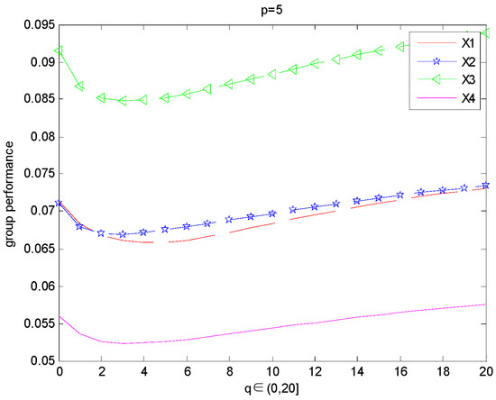
Figure 1.
The expectation of all alternatives when and .
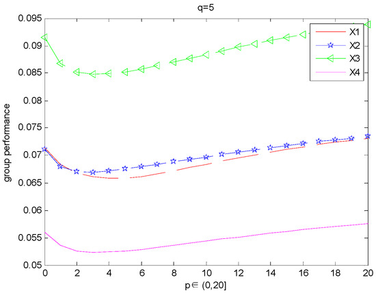
Figure 2.
The expectation of all alternatives when and .
Observing Figure 1 and Figure 2. It is not difficult to see that when or , changing another parameter from 0 to 20, the expectation curves of all attributes first drop and then rise. We can find the alternative is the best one and alternative is the worst one. When the alternative is better than alternative . And when , the alternative is the better one between and .
If we select different parameters, and change of expectation of each alternative’s IGTFWPBM operators are drawn in Figure 3, Figure 4, Figure 5 and Figure 6.
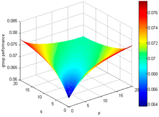
Figure 3.
Change of expectation of when .
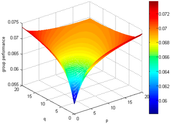
Figure 4.
Change of expectation of when .
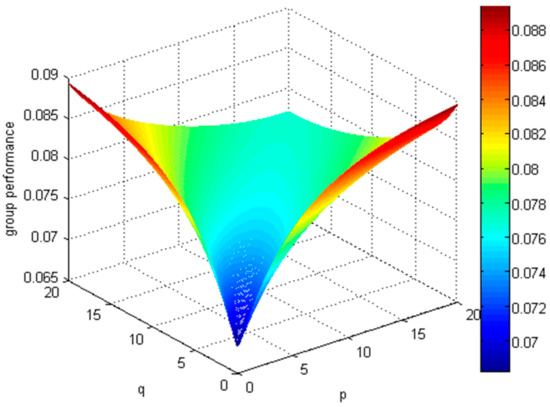
Figure 5.
Change of expectation of when .
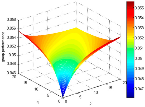
Figure 6.
Change of expectation of when .
By comparing Figure 3, Figure 4, Figure 5 and Figure 6, we find that the overall expectation level of is the highest and the overall expectation level of . The overall expectation level of and is roughly the same, but the overall fluctuation of is smaller than . In general, the parameters are larger, the decision-makers’ attitude is more positive, and the expectation of an alternative’s IGTFWPBM operator is greater.
According to Figure 3, Figure 4, Figure 5 and Figure 6, the change of expectation of four selected alternatives is symmetrical. For example, when p = 1 and q = 0, the expectation of four selected alternatives are , which is consistent with the evaluation results when p = 0 and q = 1. Therefore, in order to distinguish the differences in the hierarchical relationships among the attributes, we can adjust the unilateral parameter (p or q).
6.3. Verification of the Effectiveness
In order to further illustrate the method in more cases of applicability, new Examples 2 and 3 are used to interpret how the IGTFWPBM operators solve GFMGADM problems in the case of no relationship among attribute variables and the case of the existing relationship among attribute variables. In this section, we explain the calculation process in detail and verify the effectiveness of the decision method based on IGTFWPBM operators by comparing it with other achievements.
Example 2.
[16]: To evaluate the technological innovation ability of the four enterprisesand there are four evaluating attributes which are the ability of innovative resources investment (), the ability of innovation management (), the ability of innovation tendency (), and the ability of research and development (). There are three experts to evaluate four enterprises. Suppose thatis the expert weight vector, andis attribute weight vector, and the attribute values given by the experts take the form of interval grey triangular fuzzy numbers shown in Table 9, Table 10 and Table 11. It is worth emphasizing that in literature [16], the fuzzy part is represented by linguistic variables, we transformed linguistic variables into triangular fuzzy numbers through the transformation method [42].
Table 9.
The attribute values of each attribute to four enterprises given by expert .
Table 10.
The attribute values of each attribute to four enterprises given by expert .
Table 11.
The attribute values of each attribute to four enterprises given by expert .
We get an aggregated matrix by aggregating the assessment information which is shown in Table 12:
Table 12.
The aggregated information of each attribute to four enterprises.
Because in this case, the attribute variables are independent from each other, we divided the attribute variables into four groups, each group has only one attribute variable. Utilizing the IGTFWPBM operators to aggregate the comprehensive information of all alternatives. Suppose p = 1, q = 1, the computed result as follows:
And then, the expectation of all enterprises are
shown as follows:
Therefore, the ranking order of the four enterprises is that . Enterprise 3 is more innovative, while enterprise 4 is less innovative. In order to demonstrate the effectiveness of this method in solving the decision-making problem where there is no interrelationship among attribute variables, we selected the existing decision method with the grey fuzzy environment [16,19,20,21,22], and the comparison results are shown in Table 13.
Table 13.
Comparison of the proposed operators with other aggregation operators/methods in cases where there is no relationship among attributes.
In methods [16,19,20,21,22], the fuzzy parts are represented by linguistic variables or uncertain linguistic variables. Compared with linguistic variables and interval numbers, the fuzzy part expressed by triangular fuzzy numbers can measure the fuzziness of natural linguistic variables, which is the main distinction of a new method from existing methods. For ensuring the consistency of expert evaluation information, we used a method proposed by Liu [43] to transform the linguistic variables into the triangular fuzzy numbers. As shown in Table 13, it is not difficult to find that when there is no interrelationship among attributes, the method proposed in this paper is consistent with the decision results of the other five methods. It indicates that the IGTFWPBM operator is effective in solving the decision problem where there is no interrelationship among attribute variables. At this time, IGTFWPBM is simplified to an IGTFWBM operator, and the calculation process is relatively simple.
Example 3.
[33] ABC Nonferrous Metals Co. Ltd. is a largely state-owned company whose main business is the deep processing of nonferrous metals. In order to expand its main business, the overseas investment department decided to select a pool of alternatives from several foreign countries based on preliminary surveys. Five countrieswere evaluated through surveys and screening. Many factors affect the investment environment and four factors are chosen based on the experience of the department personnel, including: resources (such as the suitability of the minerals and their exploration);: politics and policy (such as corruption and political risks);: economy (such as development vitality and the stability); and: infrastructure (such as railway and highway facilities). The weight vector of the factors is ω = (0.25, 0.22, 0.35, 0.18). The evaluation information is shown in Table 14. There is a close correlation among the four evaluation factors. The energy reserve can influence the direction of policy formulation, and economic development depends on the resource reserve and related policies and regulations. The infrastructure depends on economic development, and the completeness of infrastructure is more conducive to the rapid development of the economy. Therefore, we classify the four attribute variables into one class for discussion.
Table 14.
The attribute values of each attribute to five countries.
Transform the assessment values into interval grey triangular fuzzy numbers, and the grey linguistic numbers [33] is replaced by , where the lower and upper bounds are equal. As independent of and , so in the process of computing and interval grey triangular fuzzy numbers can be calculated independently. And the calculation method of can be referred to the literature [16]. Utilizing the IGTFWPBM operators to aggregate the comprehensive information of all alternatives. Suppose p = 1 and q = 1, the computed result as follows:
And then, we calculate the expectation of all alternatives , for example, the calculative process of expectation is shown as follows:
And the other alternatives’ expectations are as shown below:
Therefore, the ranking of all countries is that . By comparison, we find the ranking calculated by IGTFWPBM operator is consistent with methods [16,19,33], which illustrates the effectiveness of the GFMAGDM method based on the IGTFWPBM operator. To better illustrate the superiority of the method based on the IGTFWPBM operator, we compared the existing methods in a grey fuzzy environment in Section 6.4.
6.4. Comparative Analysis
To elaborate on the validity and superiority of a new method based on the IGTFWPBM operators, we selected three examples and compared them with various methods of decision-making in the existing grey fuzzy environment [16,19,20,21,22,33]. It is not difficult to find that IGTFWPBM operators are valid in cases where there is no relation among attributes (Example 2) and a case where a simple relationship among attributes (Example 3).
To demonstrate the superiority of the proposed method, we took advantage of the decision-making problem that how to evaluate the economic development of the five countries (Example 3) to compare it with five existing grey fuzzy methods [16,19,20,21,33]. The ranking orders calculated by existing methods are represented as Table 15.
Table 15.
Comparison of the proposed operators with other aggregation operators/methods where there exits relationship among attributes.
It is worth emphasizing that to ensure the comparability of calculation methods, linguistic variables are transformed into triangular fuzzy numbers through the transformation method [43]. As shown in Table 15, the method proposed in this paper is consistent with the method that takes into account the relationship among attributes, and slightly different from the other three methods that do not capture the relationship among the attributes. This is because none of the aggregated operators consider the relationship among the attributes in methods [16,20,21], which does not conform to the decision logic in this example. The method proposed in this paper and methods [19,33] can overcome this defect and improve the accuracy of decision making.
To further illustrate the superiority of IGTFWPBM operators, two methods [19,30] that take account of attribute relationships are compared with the method in this paper according to Example 1. Furthermore, new attributes are added based on the original example, which further complicates the decision-making process. The comparison results are shown in Table 16.
Table 16.
Comparison of the proposed operators with other aggregation operators/methods where there exits interrelationship among attributes.
As shown in Table 16, when the number of attributes is 5 in the original case, the sorting results of the three methods are consistent. However, with the increasing number of attributes, the order of the SIR Choquet method [19] and GLWBM operator [33] changes. The order of the GLWBM operator fluctuates greatly. When the number of GLWBM operators increases to six attributes, the calculated order becomes ; when the attribute variable reaches eight, the permutation order becomes . The order of the SIR Choquet method changes when the number of attributes is seven, and when the number of attributes is eight, the order changes back to the original order. However, the order of IGTFWPBM operator has not changed, because IGTFWPBM operator can fully consider the interrelationship among attributes variables through classifying attributes for calculation, which greatly improves the accuracy and stability of the decision-making process. At the same time, in the calculation of IGTFWPBM operator, the decision-maker can adjust the parameters p and q to show his or her attitude towards the internal grouping relationship among attributes, which is more consistent with the actual decision-making process.
To sum up, we compare the IGTFWPBM operator with the six methods. Under the condition that the attributes are independent of each other, the calculated results of the IGTFWPBM operator are consistent with those of other methods applied in the grey fuzzy environment, indicating that the IGTFWPBM operator is effective. When there are internal relations among attributes, the method proposed in this paper considering the correlation among attributes is more accurate than the traditional grey fuzzy operator and method. When faced with more attribute variables and more complex relationships, The IGTFWPBM operator’s ability to calculate internal relationships and the setting of regulating parameters can help improve the accuracy and stability of the decision-making process, which are the notable advantages of a new method.
7. Conclusions
In this study, considering the fuzziness and greyness in real decision-making, we developed a new method for solving GFMAGDM problems. There are three main contributions to this study. In the first phase, we proposed the interval grey triangular fuzzy numbers which the grey part expressed by interval numbers and the fuzzy part in the form of triangular fuzzy numbers, after that, we gave the definitions, properties, distance, and expectations of the interval grey triangular fuzzy numbers. In the second phase, we proposed the IGTFPBM operators, combined the interval grey triangular fuzzy numbers with PBM, and gave the weighted form IGTFWPBM. The proposed operators can build the partition structure and calculate the interrelationship among the attributes. In the third phase, we developed a novel method based on IGTFWPBM. We applied the method to the example that an investment institution made decision-making to choose the best one from four small and micro-enterprises. And then, we showed the ranking results under the different parameters. The adjustment of parameters will have a symmetrical effect on the expectation of the alternative, so the importance of the variable groups can be distinguished by the unilateral adjustment of parameters. Finally, we compared the proposed method with five existing methods to illustrate the effectiveness and superiority of the new method.
In future work, we will improve the decision-making accuracy of grey fuzzy variables and apply it to high-precision medical and military fields. In terms of theoretical research, we hope to choose a more complex form to express fuzzy parts, such as Gaussian fuzzy number [44,45], intuitionistic fuzzy sets [46,47], and rough sets [48]. At the same time, BPM operators can be simplified to improve computational efficiency. On the application side, we will apply the IGTFPBM operators into more complex real-world decision cases [49,50] and further explore the application of the IGTFPBM operators in a big data environment [51].
Author Contributions
Conceptualization, K.Y.; Methodology and Writing—Original Draft, B.Y.; Formal Analysis and Writing—Review and Editing, X.J. All authors have read and agreed to the published version of the manuscript.
Funding
The paper is supported by the National Social Science Foundation of China (Grant No. 14ZDB151, No.18CJY018, No.16AZD018); the International Postdoctoral Exchange Fellowship Program (Grant No.20190023); the National Special Science Foundation for Postdoctoral Scientists of China (Grant No. 2018T110708); the National Science Foundation for Postdoctoral Scientists of China (Grant No. 2017M610446); the National Key Research and Development Program of China (Grant No. 2016YFC1402000); and the Science Foundation for Postdoctoral Scientists of Qingdao City, China (Grant No. 24).
Acknowledgments
The authors would like to thank the editors and the anonymous reviewers for their constructive comments and suggestions, which helped to improve the paper.
Conflicts of Interest
The authors declare no conflict of interest.
References
- Wang, J.; Gao, H.; Wei, G.; Wei, Y. Methods for multiple-attribute group decision making with q-rung interval-valued orthopair fuzzy information and their applications to the selection of green suppliers. Symmetry 2019, 11, 56. [Google Scholar] [CrossRef]
- Garg, H.; Kumar, K. Linguistic interval-valued atanassov intuitionistic fuzzy sets and their applications to group decision-making problems. IEEE Trans. Fuzzy Syst. 2019, 27, 2302–2311. [Google Scholar] [CrossRef]
- Wang, X.; Xu, Z.; Gou, X. Nested probabilistic-numerical linguistic term sets in two-stage multi-attribute group decision making. Appl. Intell. 2019, 49, 2582–2602. [Google Scholar] [CrossRef]
- Liu, P.D.; Gao, H. Some intuitionistic fuzzy power Bonferroni mean operators in the framework of Dempster–Shafer theory and their application to multicriteria decision making. Appl. Soft Comput. 2019, 85, 105790. [Google Scholar] [CrossRef]
- Li, Z.; Gao, H.; Wei, G. Methods for multiple attribute group decision making based on intuitionistic fuzzy Dombi Hamy mean operators. Symmetry 2018, 10, 574. [Google Scholar] [CrossRef]
- Rao, C.; Zheng, J.; Wang, C.; Xiao, X. A hybrid multi-attribute group decision making method based on grey linguistic 2-tuple. Iranian J. Fuzzy Syst. 2016, 13, 37–54. [Google Scholar]
- Rajesh, R. Group decision-making and grey programming approaches to optimal product mix in manufacturing supply chains. Neural Comput. Appl. 2018, 32, 1–15. [Google Scholar] [CrossRef]
- Song, K.; Xu, P.; Wei, G.; Chen, Y.; Wang, Q. Health management decision of sensor system based on health reliability degree and grey group decision-making. Sensors 2018, 18, 2316. [Google Scholar] [CrossRef]
- Xue, J.; Van Gelder, P.; Reniers, G.; Papadimitriou, E.; Wu, C. Multi-attribute decision-making method for prioritizing maritime traffic safety influencing factors of autonomous ships’ maneuvering decisions using grey and fuzzy theories. Saf. Sci. 2019, 120, 323–340. [Google Scholar] [CrossRef]
- Li, Q.; Diao, Y.; Gong, Z.; Hu, A. Grey language hesitant fuzzy group decision making method based on kernel and grey scale. Int. J. Environ. Res. Public Health 2018, 15, 436. [Google Scholar]
- Bu, G.Z.; Zhang, Y.W. Grey fuzzy comprehensive evaluation based on theory of grey fuzzy relation. Syst. Eng. Theory Pract. 2002, 22, 141–144. [Google Scholar]
- Luo, D.; Liu, S.F. Analytic method to a kind of grey fuzzy decision making based on entropy. Eng. Sci. 2004, 6, 48–51. [Google Scholar]
- Jin, N.; Lou, S.C. Study on multi-attribute decision making model based on the theory of grey fuzzy relation. Intell. Command Control Simul. Tech. 2004, 7, 44–47. [Google Scholar]
- Jin, N.; Lou, S.C. A grey fuzzy multi-attribute decision making method. Fire Control Command Control 2004, 29, 26–28. [Google Scholar]
- Zhu, S.Q.; Meng, K.; Zhang, H.X. Interval numbers grey fuzzy comprehensive evaluation and its application. Electron. Opt. Control. 2006, 13, 36–37. [Google Scholar]
- Jin, F.; Liu, P.D. The multi-attribute group decision making method based on the interval grey linguistic variables. Afr. J. Bus. Manag. 2010, 4, 3708–3715. [Google Scholar]
- Yin, K.; Wang, P.; Li, X. The Multi-Attribute Group Decision-Making Method Based on Interval Grey Trapezoid Fuzzy Linguistic Variable. Int. J. Environ. Res. Public Health 2017, 14, 1561. [Google Scholar] [CrossRef]
- Wang, L.; Wang, Y. Group Decision-Making Approach Based on Generalized Grey Linguistic 2-Tuple Aggregation Operators. Complexity 2018. [Google Scholar] [CrossRef]
- Wang, F.; Du, D.Y.; Zhao, J. A Novel SIR· Choquet Method for Multiple Attributes Group Decision-Making with Interval Grey Linguistic. Int. J. Fuzzy Syst. 2019, 21, 1771–1785. [Google Scholar] [CrossRef]
- Liu, P.D.; Zhang, X. Multi-attribute group decision making method based on interval grey linguistic variables weighted geometric aggregation operator. Control Decis. 2011, 24, 405–414. [Google Scholar]
- Liu, P.D. The multi-attribute group decision making method based on the interval grey linguistic variables weighted aggregation operator. J. Intell. Fuzzy Syst. 2013, 24, 405–414. [Google Scholar] [CrossRef]
- Liu, P.D.; Chu, Y.; Li, Y. The multi-attribute group decision-making method based on the interval grey uncertain linguistic generalized hybrid averaging operator. Neural Comput. Appl. 2015, 26, 1395–1405. [Google Scholar] [CrossRef]
- Bonferroni, C. Sulle medie multiple di potenze. Boll. Mat. Ital. 1950, 5, 267–270. [Google Scholar]
- Yager, R.R. On generalized Bonferroni mean operators for multi-criteria aggregation. Int. J. Approx. Reason. 2009, 50, 1279–1286. [Google Scholar] [CrossRef]
- Yager, R.R.; Beliakov, G.; James, S. On generalized Bonferroni means. In Proceedings of the Eurofuse Workshop Preference Modelling Decision Analysis, Pamplona, Spain, 16–18 September 2009; pp. 16–18. [Google Scholar]
- Beliakov, G.; James, S.; Yager, R.R. Generalized Bonferroni mean operators in multi-criteria aggregation. Fuzzy Sets Syst. 2010, 161, 2227–2242. [Google Scholar] [CrossRef]
- Wei, G.W.; Zhao, X.; Lin, R.; Wang, H. Uncertain linguistic Bonferroni mean operators and their application to multiple attribute decision making. Appl. Math. Model. 2013, 37, 5277–5285. [Google Scholar] [CrossRef]
- Jiang, X.P.; Wei, G.W. Some Bonferroni mean operators with 2-tuple linguistic information and their application to multiple attribute decision making. J. Intell. Fuzzy Syst. 2014, 27, 2153–2162. [Google Scholar] [CrossRef]
- Dutta, B.; Guha, D. Partitioned Bonferroni mean based on linguistic 2-tuple for dealing with multi-attribute group decision making. Appl. Soft Comput. 2015, 37, 166–179. [Google Scholar] [CrossRef]
- Tian, Z.P.; Wang, J.; Zhang, H.Y.; Chen, X.H.; Wang, J.Q. Simplified neutrosophic linguistic normalized weighted Bonferroni mean operator and its application to multi-criteria decision-making problems. Filomat 2016, 30, 3339–3360. [Google Scholar] [CrossRef]
- Das, S.; Guha, D.; Mesiar, R. Extended bonferroni mean under intuitionistic fuzzy environment based on a strict t-conorm. IEEE Trans. Syst. Man Cybern. Syst. 2017, 47, 2083–2099. [Google Scholar] [CrossRef]
- Liu, X.; Tao, Z.F.; Chen, H.Y.; Zhou, L.G. A new interval-valued 2-tuple linguistic Bonferroni mean operator and its application to multiattribute group decision making. Int. J. Fuzzy Syst. 2017, 19, 86–108. [Google Scholar] [CrossRef]
- Tian, Z.P.; Wang, J.; Wang, J.Q.; Chen, X.H. Multicriteria decision making approach based on gray linguistic weighted Bonferroni mean operator. Int. Trans. Oper. Res. 2018, 25, 1635–1658. [Google Scholar] [CrossRef]
- Liu, Z.M.; Liu, P.D. Intuitionistic uncertain linguistic partitioned Bonferroni means and their application to multiple attribute decision-making. Int. J. Syst. Sci. 2017, 48, 1092–1105. [Google Scholar] [CrossRef]
- Liu, P.D.; Chen, S.M.; Liu, J.L. Multiple attribute group decision making based on intuitionistic fuzzy interaction partitioned Bonferroni mean operators. Inf. Sci. 2017, 411, 98–121. [Google Scholar] [CrossRef]
- Yin, K.; Yang, B.; Li, X. Multiple attribute group decision-making methods based on Trapezoidal Fuzzy Two-Dimensional Linguistic Partitioned Bonferroni Mean Aggregation Operators. Int. J. Environ. Res. Public Health 2018, 15, 194. [Google Scholar] [CrossRef]
- Liu, P.D.; Liu, J.L. Partitioned Bonferroni mean based on two-dimensional uncertain linguistic variables for multiattribute group decision making. Int. J. Intell. Syst. 2018, 34, 1–33. [Google Scholar] [CrossRef]
- Chou, C.C. The canonical representation of multiplication operation on triangular fuzzy numbers. Comput. Math. Appl. 2003, 45, 1601–1610. [Google Scholar] [CrossRef]
- Lu, Y.; Zhang, X.B. A method for the problems of fuzzy grey multi-attribute decision-making based on the triangular fuzzy number. In Proceedings of the 2008 International Conference on Computer Science and Software Engineering, Hubei, China, 12–14 December 2008; pp. 590–593. [Google Scholar]
- Zhou, Q.; Thai, V.V. Fuzzy and grey theories in failure mode and effect analysis for tanker equipment failure prediction. Saf. Sci. 2016, 83, 74–79. [Google Scholar] [CrossRef]
- Yang, Y.; John, R. Grey sets and greyness. Inf. Sci. 2012, 185, 249–264. [Google Scholar] [CrossRef]
- Yager, R.R. OWA aggregation over a continuous interval argument with applications to decision making, IEEE Transactions on Systems. Man Cybern. Part B 2004, 34, 1952–1963. [Google Scholar] [CrossRef] [PubMed]
- Liu, P.D. A novel method for hybrid multiple attribute decision making. Knol. Based Syst. 2009, 79, 131–143. [Google Scholar]
- Wu, Q.; Law, R. Fuzzy support vector regression machine with penalizing Gaussian noises on triangular fuzzy number space. Exp. Syst. Appl. 2010, 37, 7788–7795. [Google Scholar] [CrossRef]
- Panigrahi, L.; Verma. K.; Singh, B.K. Ultrasound image segmentation using a novel multi-scale Gaussian kernel fuzzy clustering and multi-scale vector field convolution. Exp. Syst. Appl. 2019, 115, 486–498. [Google Scholar] [CrossRef]
- Xu, Z. Intuitionistic fuzzy aggregation operators. IEEE Trans. Fuzzy Syst. 2007, 15, 1179–1187. [Google Scholar]
- Garg, H.; Kumar, K. A novel exponential distance and its based TOPSIS method for interval-valued intuitionistic fuzzy sets using connection number of SPA theory. Artif. Intell. Rev. 2020, 53, 595–624. [Google Scholar] [CrossRef]
- Maldonado, S.; Peters, G.; Weber, R. Credit scoring using three-way decisions with probabilistic rough sets. Inf. Sci. 2020, 507, 700–714. [Google Scholar] [CrossRef]
- Garg, H.; Rani, D. A robust correlation coefficient measure of complex intuitionistic fuzzy sets and their applications in decision-making. Appl. Intell. 2019, 49, 496–512. [Google Scholar] [CrossRef]
- Chen, T.Y. Multiple criteria decision analysis under complex uncertainty: A Pearson-like correlation-based Pythagorean fuzzy compromise approach. Int. J. Intell. Syst. 2019, 34, 114–151. [Google Scholar] [CrossRef]
- Duan, Y.; Edwards, J.S.; Dwivedi, Y.K. Artificial intelligence for decision making in the era of Big Data–evolution, challenges and research agenda. Int. J. Inf. Manag. 2019, 48, 63–71. [Google Scholar] [CrossRef]


© 2020 by the authors. Licensee MDPI, Basel, Switzerland. This article is an open access article distributed under the terms and conditions of the Creative Commons Attribution (CC BY) license (http://creativecommons.org/licenses/by/4.0/).