A Novel Dynamic Multi-Criteria Decision Making Method Based on Generalized Dynamic Interval-Valued Neutrosophic Set

Abstract

Dynamic multi-criteria decision-making (DMCDM) models have many meaningful applications in real life in which solving indeterminacy of information in DMCDMs strengthens the potential application of DMCDM. This study introduces an extension of dynamic internal-valued neutrosophic sets namely generalized dynamic internal-valued neutrosophic sets. Based on this extension, we develop some operators and a TOPSIS method to deal with the change of both criteria, alternatives, and decision-makers by time. In addition, this study also applies the proposal model to a real application that facilitates ranking students according to attitude-skill-knowledge evaluation model. This application not only illustrates the correctness of the proposed model but also introduces its high potential appliance in the education domain.

1. Introduction

Multi-criteria decision-making (MCDM) in real world is often dynamic [1]. In the dynamic MCDM (DMCDM) model, neither alternatives nor criteria are constant throughout the whole problem and do not change over time. Besides, the DMCDM model has to cope with both dynamic and indeterminate problems of data. For example, when ranking tertiary students during learning time in a university by the set of criteria based on attitudes-skills-knowledge model (ASK), the criteria, students and lecturers are changing during semesters. The lecturers’ evaluations using scores, or other ordered scales, are also subject to indeterminacy because of lecturers’ personal experiences and biases. Therefore, a ranking model that can handle these issues is necessary.

In [2], Smarandache introduced neutrosophic set including truth-membership, an indeterminacy-membership and a falsity-membership to well treat the problem of information indeterminacy. Since then, variant forms of MCDM and DMCDM models have been proposed as in [3,4,5,6,7,8,9,10,11,12,13,14,15]. In order to consider the time dimension, Wang [16] proposed the interval neutrosophic set and its mathematical operators. Ye [9] proposed MCDM in interval-valued neutrosophic set. Dynamic MCDM for dynamic interval-valued neutrosophic set (DIVNS) was proposed in [14]. The authors have developed mathematical operators for TOPSIS method in DIVNSs.

In some cases, criteria, alternatives and decision-makers are changing by time. This fact requires a new method for DMCDM using TOPSIS method in the interval-valued neutrosophic set [17] with diversion of history data. The TOPSIS method for DIVNS in [14] did not solve the problem with the changing criteria, alternatives, and decision-makers. Liu et al. [13] combined the theory of both interval-valued neutrosophic set and hesitant fuzzy set to solve the MCDM problem. However, this study did not use TOPSIS method, and it did not consider the change of criteria also. In order to take the history data into account, Je [10] proposed two hesitant interval neutrosophic linguistic weighted operators to ranking alternatives in dynamic environment. In short, the DMCDM model in DIVNS based on TOPSIS method has not been addressed before.

The purpose of this paper is to deal with the change of criteria, alternatives, and decision-makers during time. We define generalized dynamic interval-valued neutrosophic set (GDIVNS) and some operators. Based on mathematical operators in GDIVNS (distance and weighted aggregation operators), a framework of dynamic TOPSIS is introduced. The proposed method is applied for ranking students of Thuongmai University, Vietnam on attributes of ASK model. ASK model is applicable for evaluation of tertiary students’ performance, and it gives more information that support employers besides a set of university exit benchmark. It also facilitates students to make proper self-adjustments and help them pursue appropriate professional orientation for their future career [18,19,20,21]. This application proves the suitability of the proposed model for real ranking problems.

This paper is structured as follows: The Section 1 is an introduction, and the Section 2 provides the brief preliminaries for DMCDM model in both legacy environment and interval-valued neutrosophic set. The Section 3 presents the definition of GDIVNS and some mathematical operators on this set. The Section 4 introduces the framework of dynamic TOPSIS method in GDIVNSs environment. The Section 5 presents the application of dynamic TOPSIS method in the problem of ranking students based on attributes of ASK model. The Section 6 compares the result of proposed model with previous TOPSIS model in DIVNS. The last section mentions the brief summary of this study and intended future works.

2. Preliminary

2.1. Multi-Criteria Decision-Making Model Based on History

A dynamic multi-criteria decision-making model introduced by Campanella and Ribeiro [1] is a DMCDM in which all alternatives and criteria are subject to change. The model gives decisions at all periods or just at the last one. The final rating of alternatives is calculated as:

$$E_t\left(a\right)=\{\begin{array}{ll}{R}_t\left(a\right),& a\in A_t\backslash H_{t-1}^A\\ D_E\left(E_{t-1}\left(a\right),R_t\left(a\right)\right),& a\in A_t\cap H_{t-1}^A\\ E_{t-1}\left(a\right),& a\in H_{t-1}^A\backslash A_t\end{array}$$

(1)

where $A_t$ is a set of alternatives at period $t$, $H_{t-1}^A$ is a historical set of alternatives at period $t-1$ ($H_0^A=$ Ø), $R_t\left(a\right)$ is rating of alternative $a$ at period $t$, and $D_E$ is an aggregation operator.

2.2. Dynamic Interval-Valued Neutrosophic Set and Hesitant Fuzzy Set

Thong et al. [14] introduced the concept of dynamic interval-valued neutrosophic set (DIVNS).

Definition 1.

[14] Let $U$ be a universe of discourse, and $A$ be a dynamic interval-valued neutrosophic Set (DIVNS) expressed by,

$$A=\left\{x,\langle \left[T_x^L\left(\tau \right),T_x^U\left(\tau \right)\right],\left[I_x^L\left(\tau \right),I_x^U\left(\tau \right)\right],\left[F_x^L\left(\tau \right),F_x^U\left(\tau \right)\right]\rangle |x\in U\right\}$$

(2)

where $T_x,I_x,F_x$ are the truth-membership, indeterminacy-membership, falsity-membership respectively, $\tau =\left\{{\tau }_1,{\tau }_2,\dots ,{\tau }_k\right\}$ is set of time sequence and

$$\left[T_x^L\left(\tau \right),T_x^U\left(\tau \right)\right]\subseteq \left[0,1\right]; \left[I_x^L\left(\tau \right),I_x^U\left(\tau \right)\right]\subseteq \left[0,1\right]; \left[F_x^L\left(\tau \right),F_x^U\left(\tau \right)\right]\subseteq \left[0,1\right]$$

Example 1.

A DIVNS in time sequence$\tau =\left\{{\tau }_1,{\tau }_2\right\}$and universal$U=\left\{x_1,x_2,x_3\right\}$is:

$$A=\left\{\begin{array}{l}{x}_1,\langle \left([0.5,0.6],[0.1,0.3],[0.2,0.4]\right),\left([0.4,0.55],[0.25,0.3],[0.3,0.42]\right)\rangle \\ x_2,\langle \left([0.7,0.81],[0.1,0.2],[0.1,0.2]\right),\left([0.72,0.8],[0.11,0.25],[0.2,0.4]\right)\rangle \\ x_3,\langle \left([0.3,0.5],[0.4,0.5],[0.6,0.7]\right),\left([0.4,0.5],[0.5,0.6],[0.66,0.73]\right)\rangle \end{array}\right\}$$

Hesitant fuzzy set (HFS) first introduced by Torra and Narukawa [19] and Torra [20] is defined as follows.

Definition 2.

[20] A hesitant fuzzy set E on U is defined by the function$h_E\left(x\right)$. When$h_E\left(x\right)$is applied to U, it returns a finite subset of [0, 1], which can be represented as

$$E=\left\{\langle x,h_E\left(x\right)\rangle |x\in U\right\}$$

(3)

where$h_E\left(x\right)$is a set of some values in$\left[0,1\right]$.

Example 2.

Let$X=\left\{x_1,x_2,x_3\right\}$be the discourse set, and$h_E\left(x_1\right)=\left\{0.1,0.2\right\}$,$h_E\left(x_2\right)=\left\{0.3\right\}$and$h_E\left(x_3\right)=\left\{0.2,0.3,0.5\right\}$. Then, E can be considered as a HFS:

$$E=\left\{\langle x_1,\left\{0.1,0.2\right\}\rangle ,\langle x_2,\left\{0.3\right\}\rangle ,\langle x_3,\left\{0.2,0.3,0.5\right\}\rangle \right\}$$

3. Generalized Dynamic Interval-Valued Neutrosophic Set

Extending DIVNS by the concept of HFS is considered how to express the criteria, alternatives, and DMs that are changing during time criteria, alternatives and decision-makers are changing by time.

In this section, we propose the concepts of generalized dynamic interval-valued neutrosophic set (GDIVNS) and generalized dynamic interval-valued neutrosophic element (GDIVNE) including fundamental elements, operational laws as well as the score functions. Then, GDIVNS’s theory is applied for the decision-making model in Section 4.

Definition 3.

Let U be a universe of discourse. A generalized dynamic interval-valued neutrosophic set (GDIVNS) in U can be expressed as,

$$\tilde{E}=\left\{\langle x,{\tilde{h}}_{\tilde{E}}\left(x\left(t_r\right)\right)\rangle |x\in U;\forall t_r\in t;\right\}$$

(4)

where${\tilde{h}}_{\tilde{E}}\left(x\left(t_r\right)\right)$is expressed for importing HFS into DIVNS.${\tilde{h}}_{\tilde{E}}\left(x\left(t_r\right)\right)$is a set of DIVNSs at period$t_r$and$t=\left\{t_1,t_2,t_3,\dots ,t_s\right\}$, which denotes the possible DIVNSs of the element$x\in X$to the set$\tilde{E}$,${\tilde{h}}_{\tilde{E}}\left(x\left(t_r\right)\right)$can be represented by a generalized dynamic interval-valued neutrosophic element (GDIVNE). When$s=1$and$\left|{\tilde{h}}_{\tilde{E}}\left(x\left(t_r\right)\right)\right|=1$, GDIVNS simplifies to DIVNS [14]. For convenience, we denote$\tilde{h}={\tilde{h}}_{\tilde{E}}\left(x\left(t\right)\right)=\left\{\gamma |\gamma \in \tilde{h}\right\}$, where

$$\gamma =\left(\left[T_{}^L\left(x\left(\tau \right)\right),T_{}^U\left(x\left(\tau \right)\right)\right],\left[I_{}^L\left(x\left(\tau \right)\right),I_{}^U\left(x\left(\tau \right)\right)\right],\left[F_{}^L\left(x\left(\tau \right)\right),F_{}^U\left(x\left(\tau \right)\right)\right]\right)$$

is a dynamic interval-valued neutrosophic number.

Example 3.

Let$t=\left\{t_1,t_2\right\}$;$\tau =\left\{{\tau }_1,{\tau }_2\right\}$and an universal$X=\left\{x_1,x_2,x_3\right\}$. A GDIVNS in$X$is given as:

$$\tilde{E}=\left\{\begin{array}{l}\langle x_1,\left\{\begin{array}{l}\langle \left([0.2,0.33],[0.4,0.5],[0.6,0.7]\right),\left([0.24,0.39],[0.38,0.47],[0.56,0.7]\right)\rangle ,\\ \langle \left([0.29,0.37],[0.3,0.5],[0.4,0.58]\right),\left([0.4,0.5],[0.2,0.3],[0.35,0.42]\right)\rangle \end{array}\right\}\rangle ,\\ \langle x_2,\left\{\begin{array}{l}\langle \left([0.8,0.9],[0.1,0.2],[0.1,0.2]\right),\left([0.72,0.8],[0.11,0.25],[0.23,0.45]\right)\rangle ,\\ \langle \left([0.4,0.6],[0.2,0.4],[0.3,0.4]\right),\left([0.41,0.5],[0.26,0.39],[0.2,0.3]\right)\rangle \end{array}\right\}\rangle ,\\ \langle x_3,\left\{\begin{array}{l}\langle \left([0.6,0.7],[0.2,0.3],[0.4,0.5]\right),\left([0.52,0.66],[0.34,0.4],[0.6,0.77]\right)\rangle ,\\ \langle \left([0.54,0.62],[0.15,0.3],[0.2,0.4]\right),\left([0.4,0.5],[0.25,0.32],[0.39,0.43]\right)\rangle \end{array}\right\}\rangle \end{array}\right\}$$

Definition 4.

Let$\tilde{h}$,${\tilde{h}}_1$and${\tilde{h}}_2$be three GDIVNEs. When$\lambda >0$, the operations of GDIVNEs are defined as follows:

(i)

Addition

$$\begin{array}{l}{\tilde{h}}_1\oplus {\tilde{h}}_2={\displaystyle {\cup }_{\forall {\gamma }_1\in {\tilde{h}}_1;\forall {\gamma }_2\in {\tilde{h}}_2}\left\{{\gamma }_1\oplus {\gamma }_2\right\}}\\ =\left\{\langle \begin{array}{l}\left[T_{{\gamma }_1}^L\left(x\left(\tau \right)\right)+T_{{\gamma }_2}^L\left(x\left(\tau \right)\right)-T_{{\gamma }_1}^L\left(x\left(\tau \right)\right)\times T_{{\gamma }_2}^L\left(x\left(\tau \right)\right),T_{{\gamma }_1}^U\left(x\left(\tau \right)\right)+T_{{\gamma }_2}^U\left(x\left(\tau \right)\right)-T_{{\gamma }_1}^U\left(x\left(\tau \right)\right)\times T_{{\gamma }_2}^U\left(x\left(\tau \right)\right)\right],\\ \left[I_{{\gamma }_1}^L\left(x\left(\tau \right)\right)\times I_{{\gamma }_2}^L\left(x\left(\tau \right)\right),I_{{\gamma }_1}^U\left(x\left(\tau \right)\right)\times I_{{\gamma }_2}^U\left(x\left(\tau \right)\right)\right],\left[F_{{\gamma }_1}^L\left(x\left(\tau \right)\right)\times F_{{\gamma }_2}^L\left(x\left(\tau \right)\right),F_{{\gamma }_1}^U\left(x\left(\tau \right)\right)\times F_{{\gamma }_2}^U\left(x\left(\tau \right)\right)\right]\end{array}\rangle \right\}\end{array}$$

(ii)

Multiplication

$$\begin{array}{l}{\tilde{h}}_1\otimes {\tilde{h}}_2={\displaystyle {\cup }_{\forall {\gamma }_1\in {\tilde{h}}_1;\forall {\gamma }_2\in {\tilde{h}}_2}\left\{{\gamma }_1\otimes {\gamma }_2\right\}}\\ =\left\{\langle \begin{array}{l}\left[T_{{\gamma }_1}^L\left(x\left(\tau \right)\right)\times T_{{\gamma }_2}^L\left(x\left(\tau \right)\right),T_{{\gamma }_1}^U\left(x\left(\tau \right)\right)\times T_{{\gamma }_2}^U\left(x\left(\tau \right)\right)\right],\\ \left[I_{{\gamma }_1}^L\left(x\left(\tau \right)\right)+I_{{\gamma }_2}^L\left(x\left(\tau \right)\right)-I_{{\gamma }_1}^L\left(x\left(\tau \right)\right)\times I_{{\gamma }_2}^L\left(x\left(\tau \right)\right),I_{{\gamma }_1}^U\left(x\left(\tau \right)\right)+I_{{\gamma }_2}^U\left(x\left(\tau \right)\right)-I_{{\gamma }_1}^U\left(x\left(\tau \right)\right)\times I_{{\gamma }_2}^U\left(x\left(\tau \right)\right)\right],\\ \left[F_{{\gamma }_1}^L\left(x\left(\tau \right)\right)+F_{{\gamma }_2}^L\left(x\left(\tau \right)\right)-F_{{\gamma }_1}^L\left(x\left(\tau \right)\right)\times F_{{\gamma }_2}^L\left(x\left(\tau \right)\right),F_{{\gamma }_1}^U\left(x\left(\tau \right)\right)+F_{{\gamma }_2}^U\left(x\left(\tau \right)\right)-F_{{\gamma }_1}^U\left(x\left(\tau \right)\right)\times F_{{\gamma }_2}^U\left(x\left(\tau \right)\right)\right]\end{array}\rangle \right\}\end{array}$$

(iii)

Scalar Multiplication

$$\begin{array}{l}\lambda \tilde{h}={\displaystyle {\cup }_{\forall \gamma \in \tilde{h}}\left\{\lambda \gamma \right\}}\\ ={\displaystyle {\cup }_{\forall \gamma \in \tilde{h}}\left\{\langle \begin{array}{l}\left[1-{\left(1-T^L\left(x\left(\tau \right)\right)\right)}^{\lambda },1-{\left(1-T^U\left(x\left(\tau \right)\right)\right)}^{\lambda }\right],\\ \left[{\left(I^L\left(x\left(\tau \right)\right)\right)}^{\lambda },{\left(I^U\left(x\left(\tau \right)\right)\right)}^{\lambda }\right],\left[{\left(F^L\left(x\left(\tau \right)\right)\right)}^{\lambda },{\left(F^U\left(x\left(\tau \right)\right)\right)}^{\lambda }\right]\end{array}\rangle \right\}}\end{array}$$

(iv)

Power

$$\begin{array}{l}{\tilde{h}}^{\lambda }={\displaystyle {\cup }_{\forall \gamma \in \tilde{h}}\left\{{\gamma }^{\lambda }\right\}}\\ ={\displaystyle {\cup }_{\forall \gamma \in \tilde{h}}\left\{\langle \begin{array}{l}\left[{\left(T^L\left(x\left(\tau \right)\right)\right)}^{\lambda },{\left(T^U\left(x\left(\tau \right)\right)\right)}^{\lambda }\right],\left[1-{\left(1-I^L\left(x\left(\tau \right)\right)\right)}^{\lambda },1-{\left(1-I^U\left(x\left(\tau \right)\right)\right)}^{\lambda }\right],\\ \left[1-{\left(1-F^L\left(x\left(\tau \right)\right)\right)}^{\lambda },1-{\left(1-F^U\left(x\left(\tau \right)\right)\right)}^{\lambda }\right]\end{array}\rangle \right\}}\end{array}$$

Definition 5.

Let$\tilde{h}$be a GDIVNE. Then, the score functions of the GDIVNE$\tilde{h}$are defined by,

$$S\left(\tilde{h}\right)=\frac{1}{\#\tilde{h}}\times \frac{1}{k}{\displaystyle \sum _{\forall \gamma \in \tilde{h}}{\displaystyle \sum _{l=1}^k\left(\left(\frac{T^L\left({\tau }_l\right)+T^U\left({\tau }_l\right)}{2}+\left(1-\frac{I^L\left({\tau }_l\right)+I^U\left({\tau }_l\right)}{2}\right)+\left(1-\frac{F^L\left({\tau }_l\right)+F^U\left({\tau }_l\right)}{2}\right)\right)/3\right)}}$$

(5)

where$\tau =\left\{{\tau }_1,{\tau }_2,\dots ,{\tau }_k\right\}$, and$\#\tilde{h}$is number of elements in$\tilde{h}$. Obviously,$S\left(\tilde{h}\right)\in \left[0,1\right]$. If$S\left({\tilde{h}}_1\right)\ge S\left({\tilde{h}}_2\right)$, then${\tilde{h}}_1\ge {\tilde{h}}_2$.

Example 4.

Let three GDIVNEs:

$$\begin{array}{l}{\tilde{h}}_1=\left\{\langle \left([1,1],[0,0],[0,0]\right),\left([1,1],[0,0],[0,0]\right)\rangle ,\langle \left([1,1],[0,0],[0,0]\right),\left([1,1],[0,0],[0,0]\right)\rangle \right\}\\ {\tilde{h}}_2=\left\{\langle \left([0,0],[1,1],[0,0]\right),\left([0,0],[1,1],[0,0]\right)\rangle ,\langle \left([0,0],[1,1],[0,0]\right),\left([0,0],[1,1],[0,0]\right)\rangle \right\}\\ {\tilde{h}}_3=\left\{\langle \left([0,0],[1,1],[1,1]\right),\left([0,0],[1,1],[1,1]\right)\rangle ,\langle \left([0,0],[1,1],[1,1]\right),\left([0,0],[1,1],[1,1]\right)\rangle \right\}\end{array}$$

According to Equation (5), we have $S\left({\tilde{h}}_1\right)=1; S\left({\tilde{h}}_2\right)=\frac{1}{3}; S\left({\tilde{h}}_3\right)=0$. Thus, ${\tilde{h}}_1>{\tilde{h}}_2>{\tilde{h}}_3$.

Definition 6.

Let${\tilde{h}}_j\left(j=1,2,\dots ,n\right)$be a collection of GDIVNEs. Generalized dynamic interval-valued neutrosophic weighted average (GDIVNWA) operator is defined as

$$\begin{array}{l}GDIVNWA\left({\tilde{h}}_1,{\tilde{h}}_2,\dots ,{\tilde{h}}_n\right)={\displaystyle \sum _{j=1}^n{w}_j{\tilde{h}}_j}\\ ={\displaystyle \underset{{\gamma }_1\in {\tilde{h}}_1,{\gamma }_2\in {\tilde{h}}_2,\dots ,{\gamma }_n\in {\tilde{h}}_n}{\cup }\left\{\left(\begin{array}{l}\left[1-{\displaystyle \prod _{j=1}^n{\left(1-T_{{\gamma }_j}^L\left(\tau \right)\right)}^{w_j}},1-{\displaystyle \prod _{j=1}^n{\left(1-T_{{\gamma }_j}^U\left(\tau \right)\right)}^{w_j}}\right],\\ \left[{\displaystyle \prod _{j=1}^n{\left(I_{{\gamma }_j}^L\left(\tau \right)\right)}^{w_j},}{\displaystyle \prod _{j=1}^n{\left(I_{{\gamma }_j}^U\left(\tau \right)\right)}^{w_j}}\right],\left[{\displaystyle \prod _{j=1}^n{\left(F_{{\gamma }_j}^L\left(\tau \right)\right)}^{w_j},}{\displaystyle \prod _{j=1}^n{\left(F_{{\gamma }_j}^U\left(\tau \right)\right)}^{w_j}}\right]\end{array}\right)\right\}}\end{array}$$

(6)

Theorem 1.

Let${\tilde{h}}_j\left(j=1,2,\dots ,n\right)$be the collection of GDIVNEs. The result aggregated from GDIVNWA operator is still a GDIVNE.

Proof. 

The Equation (6) is proved by mathematical inductive reasoning method. □

When $n=1$, Equation (6) holds because it simplifies to the trivial outcome, which is obviously GDIVNE as,

$$GDIVNWA\left({\tilde{h}}_1\right)=\left(\begin{array}{l}\left[1-{\left(1-T_{{\gamma }_1}^L\left(\tau \right)\right)}^{w_1},1-{\left(1-T_{{\gamma }_1}^U\left(\tau \right)\right)}^{w_1}\right],\\ \left[{\left(I_{{\gamma }_1}^L\left(\tau \right)\right)}^{w_1},{\left(I_{{\gamma }_1}^U\left(\tau \right)\right)}^{w_1}\right],\left[{\left(F_{{\gamma }_1}^L\left(\tau \right)\right)}^{w_1},{\left(F_{{\gamma }_1}^U\left(\tau \right)\right)}^{w_1}\right]\end{array}\right)$$

(7)

Let us assume that (6) is true for $n=z$,

$${\displaystyle \sum _{j=1}^z{w}_j{\tilde{h}}_j}={\displaystyle \underset{{\gamma }_1\in {\tilde{h}}_1,{\gamma }_2\in {\tilde{h}}_2,\dots ,{\gamma }_z\in {\tilde{h}}_z}{\cup }\left\{\left(\begin{array}{l}\left[1-{\displaystyle \prod _{j=1}^z{\left(1-T_{{\gamma }_j}^L\left(\tau \right)\right)}^{w_j}},1-{\displaystyle \prod _{j=1}^z{\left(1-T_{{\gamma }_j}^U\left(\tau \right)\right)}^{w_j}}\right],\\ \left[{\displaystyle \prod _{j=1}^z{\left(I_{{\gamma }_j}^L\left(\tau \right)\right)}^{w_j},}{\displaystyle \prod _{j=1}^z{\left(I_{{\gamma }_j}^U\left(\tau \right)\right)}^{w_j}}\right],\left[{\displaystyle \prod _{j=1}^z{\left(F_{{\gamma }_j}^L\left(\tau \right)\right)}^{w_j},}{\displaystyle \prod _{j=1}^z{\left(F_{{\gamma }_j}^U\left(\tau \right)\right)}^{w_j}}\right]\end{array}\right)\right\}}$$

(8)

When $n=z+1$

$$\begin{array}{l}{\displaystyle \sum _{j=1}^{z+1}{w}_j{\tilde{h}}_j}={\displaystyle \sum _{j=1}^z{w}_j{\tilde{h}}_j\oplus w_{z+1}{\tilde{h}}_{z+1}}\\ ={\displaystyle \underset{{\gamma }_1\in {\tilde{h}}_1,{\gamma }_2\in {\tilde{h}}_2,\dots ,{\gamma }_z\in {\tilde{h}}_z}{\cup }\left\{\left(\begin{array}{l}\left[1-{\displaystyle \prod _{j=1}^z{\left(1-T_{{\gamma }_j}^L\left(\tau \right)\right)}^{w_j}},1-{\displaystyle \prod _{j=1}^z{\left(1-T_{{\gamma }_j}^U\left(\tau \right)\right)}^{w_j}}\right],\\ \left[{\displaystyle \prod _{j=1}^z{\left(I_{{\gamma }_j}^L\left(\tau \right)\right)}^{w_j},}{\displaystyle \prod _{j=1}^z{\left(I_{{\gamma }_j}^U\left(\tau \right)\right)}^{w_j}}\right],\left[{\displaystyle \prod _{j=1}^z{\left(F_{{\gamma }_j}^L\left(\tau \right)\right)}^{w_j},}{\displaystyle \prod _{j=1}^z{\left(F_{{\gamma }_j}^U\left(\tau \right)\right)}^{w_j}}\right]\end{array}\right)\right\}}\\ \oplus \left(\begin{array}{l}\left[1-{\left(1-T_{{\gamma }_{k+1}}^L\left(\tau \right)\right)}^{w_{z+1}},1-{\left(1-T_{{\gamma }_{z+1}}^U\left(\tau \right)\right)}^{w_{z+1}}\right],\\ \left[{\left(I_{{\gamma }_{z+1}}^L\left(\tau \right)\right)}^{w_{z+1}},{\left(I_{{\gamma }_{z+1}}^U\left(\tau \right)\right)}^{w_{z+1}}\right],\left[{\left(F_{{\gamma }_{z+1}}^L\left(\tau \right)\right)}^{w_{z+1}},{\left(F_{{\gamma }_{z+1}}^U\left(\tau \right)\right)}^{w_{z+1}}\right]\end{array}\right)\\ ={\displaystyle \underset{{\gamma }_1\in {\tilde{h}}_1,{\gamma }_2\in {\tilde{h}}_2,\dots ,{\gamma }_{z+1}\in {\tilde{h}}_{z+1}}{\cup }\left\{\left(\begin{array}{l}\left[1-{\displaystyle \prod _{j=1}^{z+1}{\left(1-T_{{\gamma }_j}^L\left(\tau \right)\right)}^{w_j}},1-{\displaystyle \prod _{j=1}^{z+1}{\left(1-T_{{\gamma }_j}^U\left(\tau \right)\right)}^{w_j}}\right],\\ \left[{\displaystyle \prod _{j=1}^{z+1}{\left(I_{{\gamma }_j}^L\left(\tau \right)\right)}^{w_j},}{\displaystyle \prod _{j=1}^{z+1}{\left(I_{{\gamma }_j}^U\left(\tau \right)\right)}^{w_j}}\right],\left[{\displaystyle \prod _{j=1}^{z+1}{\left(F_{{\gamma }_j}^L\left(\tau \right)\right)}^{w_j},}{\displaystyle \prod _{j=1}^{z+1}{\left(F_{{\gamma }_j}^U\left(\tau \right)\right)}^{w_j}}\right]\end{array}\right)\right\}}\end{array}$$

(9)

It follows that if (6) holds for $n=z$, then it holds for $n=z+1$. Because it is also true for $n=1$, according to the method of mathematical inductive reasoning, Equation (6) holds for natural numbers N and Theorem 1 is proven.

Definition 7.

Let${\tilde{h}}_j\left(j=1,2,\dots ,n\right)$be a collection of GDIVNEs. Generalized dynamic interval-valued neutrosophic weighted geometric (GDIVNWG) operator is defined as

$$\begin{array}{l}GDIVNWG\left({\tilde{h}}_1,{\tilde{h}}_2,\dots ,{\tilde{h}}_n\right)={\displaystyle \prod _{j=1}^n{\tilde{h}}_j^{w_j}}\\ ={\displaystyle \underset{{\gamma }_1\in {\tilde{h}}_1,{\gamma }_2\in {\tilde{h}}_2,\dots ,{\gamma }_n\in {\tilde{h}}_n}{\cup }\left\{\left(\begin{array}{l}\left[{\displaystyle \prod _{j=1}^n{\left(T_{{\gamma }_j}^L\left(\tau \right)\right)}^{w_j},}{\displaystyle \prod _{j=1}^n{\left(T_{{\gamma }_j}^U\left(\tau \right)\right)}^{w_j}}\right],\left[1-{\displaystyle \prod _{j=1}^n{\left(1-I_{{\gamma }_j}^L\left(\tau \right)\right)}^{w_j}},1-{\displaystyle \prod _{j=1}^n{\left(1-I_{{\gamma }_j}^U\left(\tau \right)\right)}^{w_j}}\right],\\ \left[1-{\displaystyle \prod _{j=1}^n{\left(1-F_{{\gamma }_j}^L\left(\tau \right)\right)}^{w_j}},1-{\displaystyle \prod _{j=1}^n{\left(1-F_{{\gamma }_j}^U\left(\tau \right)\right)}^{w_j}}\right]\end{array}\right)\right\}}\end{array}$$

(10)

Theorem 2.

Let${\tilde{h}}_j\left(j=1,2,\dots ,n\right)$be the collection of GDIVNEs. The result aggregated from GDIVNWG operator is still a GDIVNE.

Proof. 

The Equation (10) is proved by mathematical inductive reasoning method. □

When $n=1$, Equation (10) is true because it simplifies to the trivial outcome, which is obviously GDIVNE,

$$GDIVNWG\left({\tilde{h}}_1\right)=\left(\begin{array}{l}\left[{\left(T_{{\gamma }_1}^L\left(\tau \right)\right)}^{w_1},{\left(T_{{\gamma }_1}^U\left(\tau \right)\right)}^{w_1}\right],\left[1-{\left(1-I_{{\gamma }_1}^L\left(\tau \right)\right)}^{w_1},1-{\left(1-I_{{\gamma }_1}^U\left(\tau \right)\right)}^{w_1}\right],\\ \left[1-{\left(1-F_{{\gamma }_1}^L\left(\tau \right)\right)}^{w_1},1-{\left(1-F_{{\gamma }_1}^U\left(\tau \right)\right)}^{w_1}\right]\end{array}\right)$$

(11)

Let us assume that (10) is true for $n=z$.

$${\displaystyle \prod _{j=1}^z{\tilde{h}}_j^{w_j}}={\displaystyle \underset{{\gamma }_1\in {\tilde{h}}_1,{\gamma }_2\in {\tilde{h}}_2,\dots ,{\gamma }_z\in {\tilde{h}}_z}{\cup }\left\{\left(\begin{array}{l}\left[{\displaystyle \prod _{j=1}^z{\left(T_{{\gamma }_j}^L\left(\tau \right)\right)}^{w_j},}{\displaystyle \prod _{j=1}^z{\left(T_{{\gamma }_j}^U\left(\tau \right)\right)}^{w_j}}\right],\left[1-{\displaystyle \prod _{j=1}^z{\left(1-I_{{\gamma }_j}^L\left(\tau \right)\right)}^{w_j}},1-{\displaystyle \prod _{j=1}^z{\left(1-I_{{\gamma }_j}^U\left(\tau \right)\right)}^{w_j}}\right],\\ \left[1-{\displaystyle \prod _{j=1}^z{\left(1-F_{{\gamma }_j}^L\left(\tau \right)\right)}^{w_j}},1-{\displaystyle \prod _{j=1}^z{\left(1-F_{{\gamma }_j}^U\left(\tau \right)\right)}^{w_j}}\right]\end{array}\right)\right\}}$$

(12)

When $n=z+1$

$$\begin{array}{l}{\displaystyle \prod _{j=1}^{z+1}{\tilde{h}}_j^{w_j}}={\displaystyle \prod _{j=1}^z{\tilde{h}}_j^{w_j}}\otimes {\tilde{h}}_{z+1}^{w_{z+1}}\\ ={\displaystyle \underset{{\gamma }_1\in {\tilde{h}}_1,{\gamma }_2\in {\tilde{h}}_2,\dots ,{\gamma }_z\in {\tilde{h}}_z}{\cup }\left\{\left(\begin{array}{l}\left[{\displaystyle \prod _{j=1}^k{\left(T_{{\gamma }_j}^L\left(\tau \right)\right)}^{w_j},}{\displaystyle \prod _{j=1}^k{\left(T_{{\gamma }_j}^U\left(\tau \right)\right)}^{w_j}}\right],\left[1-{\displaystyle \prod _{j=1}^k{\left(1-I_{{\gamma }_j}^L\left(\tau \right)\right)}^{w_j}},1-{\displaystyle \prod _{j=1}^k{\left(1-I_{{\gamma }_j}^U\left(\tau \right)\right)}^{w_j}}\right],\\ \left[1-{\displaystyle \prod _{j=1}^k{\left(1-F_{{\gamma }_j}^L\left(\tau \right)\right)}^{w_j}},1-{\displaystyle \prod _{j=1}^k{\left(1-F_{{\gamma }_j}^U\left(\tau \right)\right)}^{w_j}}\right]\end{array}\right)\right\}}\\ \otimes \left(\begin{array}{l}\left[{\left(T_{{\gamma }_j}^L\left(\tau \right)\right)}^{w_{z+1}},{\left(T_{{\gamma }_{z+1}}^U\left(\tau \right)\right)}^{w_{z+1}}\right],\left[1-{\left(1-I_{{\gamma }_{z+1}}^L\left(\tau \right)\right)}^{w_{z+1}},1-{\left(1-I_{{\gamma }_{z+1}}^U\left(\tau \right)\right)}^{w_{z+1}}\right],\\ \left[1-{\left(1-F_{{\gamma }_{z+1}}^L\left(\tau \right)\right)}^{w_{z+1}},1-{\left(1-F_{{\gamma }_{z+1}}^U\left(\tau \right)\right)}^{w_{z+1}}\right]\end{array}\right)\\ ={\displaystyle \underset{{\gamma }_1\in {\tilde{h}}_1,{\gamma }_2\in {\tilde{h}}_2,\dots ,{\gamma }_{z+1}\in {\tilde{h}}_{z+1}}{\cup }\left\{\left(\begin{array}{l}\left[{\displaystyle \prod _{j=1}^{z+1}{\left(T_{{\gamma }_j}^L\left(\tau \right)\right)}^{w_j},}{\displaystyle \prod _{j=1}^{z+1}{\left(T_{{\gamma }_j}^U\left(\tau \right)\right)}^{w_j}}\right],\left[1-{\displaystyle \prod _{j=1}^{z+1}{\left(1-I_{{\gamma }_j}^L\left(\tau \right)\right)}^{w_j}},1-{\displaystyle \prod _{j=1}^{z+1}{\left(1-I_{{\gamma }_j}^U\left(\tau \right)\right)}^{w_j}}\right],\\ \left[1-{\displaystyle \prod _{j=1}^{z+1}{\left(1-F_{{\gamma }_j}^L\left(\tau \right)\right)}^{w_j}},1-{\displaystyle \prod _{j=1}^{z+1}{\left(1-F_{{\gamma }_j}^U\left(\tau \right)\right)}^{w_j}}\right]\end{array}\right)\right\}}\end{array}$$

(13)

It follows that if (10) holds for $n=z$, then it holds for $n=z+1$. Because it is also true for $n=1$, according to the method of mathematical inductive reasoning, Equation (10) holds for all natural numbers N and Theorem 2 is proven.

Herein, we define the generalized dynamic interval-valued neutrosophic hybrid weighted averaging (GDIVNHWA) operator to combine the effects of attribute weight vector and the positional weight vector, which are mentioned in Definitions 6 and 7.

Definition 8.

Let$\lambda >0$and${\tilde{h}}_j\left(j=1,2,\dots ,n\right)$be a collection of GDIVNEs. Generalized dynamic interval-valued neutrosophic hybrid weighted averaging (GDIVNHWA) operator is defined as,

$$\begin{array}{l}DIVHNWG\left({\tilde{h}}_1,{\tilde{h}}_2,\dots ,{\tilde{h}}_n\right)={\left({\displaystyle \sum _{j=1}^n{w}_j{\tilde{h}}_j^{\lambda }}\right)}^{\raisebox{1ex}{$1$}\!\left/ \!\raisebox{-1ex}{$\lambda $}\right.}\\ ={\displaystyle \underset{{\gamma }_1\in {\tilde{h}}_1,{\gamma }_2\in {\tilde{h}}_2,\dots ,{\gamma }_n\in {\tilde{h}}_n}{\cup }\left\{\left(\begin{array}{l}\left[{\left(1-{\displaystyle \prod _{j=1}^n{\left(1-{\left(T_{{\gamma }_j}^L\left(\tau \right)\right)}^{\lambda }\right)}^{w_j}}\right)}^{\raisebox{1ex}{$1$}\!\left/ \!\raisebox{-1ex}{$\lambda $}\right.},{\left(1-{\displaystyle \prod _{j=1}^n{\left(1-{\left(T_{{\gamma }_j}^U\left(\tau \right)\right)}^{\lambda }\right)}^{w_j}}\right)}^{\raisebox{1ex}{$1$}\!\left/ \!\raisebox{-1ex}{$\lambda $}\right.}\right],\\ \left[1-{\left(1-{\displaystyle \prod _{j=1}^n{\left(1-{\left(1-I_{{\gamma }_j}^L\left(\tau \right)\right)}^{\lambda }\right)}^{w_j}}\right)}^{\raisebox{1ex}{$1$}\!\left/ \!\raisebox{-1ex}{$\lambda $}\right.},1-{\left(1-{\displaystyle \prod _{j=1}^n{\left(1-{\left(1-I_{{\gamma }_j}^U\left(\tau \right)\right)}^{\lambda }\right)}^{w_j}}\right)}^{\raisebox{1ex}{$1$}\!\left/ \!\raisebox{-1ex}{$\lambda $}\right.}\right],\\ \left[1-{\left(1-{\displaystyle \prod _{j=1}^n{\left(1-{\left(1-F_{{\gamma }_j}^L\left(\tau \right)\right)}^{\lambda }\right)}^{w_j}}\right)}^{\raisebox{1ex}{$1$}\!\left/ \!\raisebox{-1ex}{$\lambda $}\right.},1-{\left(1-{\displaystyle \prod _{j=1}^n{\left(1-{\left(1-F_{{\gamma }_j}^U\left(\tau \right)\right)}^{\lambda }\right)}^{w_j}}\right)}^{\raisebox{1ex}{$1$}\!\left/ \!\raisebox{-1ex}{$\lambda $}\right.}\right]\end{array}\right)\right\}}\end{array}$$

(14)

Theorem 3.

Let${\tilde{h}}_j\left(j=1,2,\dots ,n\right)$be the collection of GDIVNEs. The result aggregated from GDIVNHWA operator is still a GDIVNE.

Proof. 

The Equation (14) can be proved by mathematical inductive reasoning method. □

We first prove that (15) is a collection of GDIVNEs,

$${\displaystyle \sum _{j=1}^n{w}_j{\tilde{h}}_j^{\lambda }}={\displaystyle \underset{{\gamma }_1\in {\tilde{h}}_1,{\gamma }_2\in {\tilde{h}}_2,\dots ,{\gamma }_n\in {\tilde{h}}_n}{\cup }\left\{\left(\begin{array}{l}\left[1-{\displaystyle \prod _{j=1}^n{\left(1-{\left(T_{{\gamma }_j}^L\left(\tau \right)\right)}^{\lambda }\right)}^{w_j}},1-{\displaystyle \prod _{j=1}^n{\left(1-{\left(T_{{\gamma }_j}^U\left(\tau \right)\right)}^{\lambda }\right)}^{w_j}}\right],\\ \left[1-{\displaystyle \prod _{j=1}^n{\left(1-{\left(1-I_{{\gamma }_j}^L\left(\tau \right)\right)}^{\lambda }\right)}^{w_j}},1-{\displaystyle \prod _{j=1}^n{\left(1-{\left(1-I_{{\gamma }_j}^U\left(\tau \right)\right)}^{\lambda }\right)}^{w_j}}\right],\\ \left[1-{\displaystyle \prod _{j=1}^n{\left(1-{\left(1-F_{{\gamma }_j}^L\left(\tau \right)\right)}^{\lambda }\right)}^{w_j}},1-{\displaystyle \prod _{j=1}^n{\left(1-{\left(1-F_{{\gamma }_j}^U\left(\tau \right)\right)}^{\lambda }\right)}^{w_j}}\right]\end{array}\right)\right\}}$$

(15)

When $n=1$, Equation (15) is true because it simplifies to the trivial outcome, which is obviously GDIVNE,

$$w_1{\tilde{h}}_1^{\lambda }=\left(\begin{array}{l}\left[1-{\left(1-{\left(T_{{\gamma }_1}^L\left(\tau \right)\right)}^{\lambda }\right)}^{w_1},1-{\left(1-{\left(T_{{\gamma }_1}^U\left(\tau \right)\right)}^{\lambda }\right)}^{w_1}\right],\\ \left[1-{\left(1-{\left(1-I_{{\gamma }_1}^L\left(\tau \right)\right)}^{\lambda }\right)}^{w_1},1-{\left(1-{\left(1-I_{{\gamma }_1}^U\left(\tau \right)\right)}^{\lambda }\right)}^{w_1}\right],\\ \left[1-{\left(1-{\left(1-F_{{\gamma }_1}^L\left(\tau \right)\right)}^{\lambda }\right)}^{w_1},1-{\left(1-{\left(1-F_{{\gamma }_1}^U\left(\tau \right)\right)}^{\lambda }\right)}^{w_1}\right]\end{array}\right)$$

(16)

Let us assume that (15) is true for $n=z$,

$${\displaystyle \sum _{j=1}^z{w}_j{\tilde{h}}_j^{\lambda }}={\displaystyle \underset{{\gamma }_1\in {\tilde{h}}_1,{\gamma }_2\in {\tilde{h}}_2,\dots ,{\gamma }_z\in {\tilde{h}}_z}{\cup }\left\{\left(\begin{array}{l}\left[1-{\displaystyle \prod _{j=1}^z{\left(1-{\left(T_{{\gamma }_j}^L\left(\tau \right)\right)}^{\lambda }\right)}^{w_j}},1-{\displaystyle \prod _{j=1}^z{\left(1-{\left(T_{{\gamma }_j}^U\left(\tau \right)\right)}^{\lambda }\right)}^{w_j}}\right],\\ \left[1-{\displaystyle \prod _{j=1}^z{\left(1-{\left(1-I_{{\gamma }_j}^L\left(\tau \right)\right)}^{\lambda }\right)}^{w_j}},1-{\displaystyle \prod _{j=1}^z{\left(1-{\left(1-I_{{\gamma }_j}^U\left(\tau \right)\right)}^{\lambda }\right)}^{w_j}}\right],\\ \left[1-{\displaystyle \prod _{j=1}^z{\left(1-{\left(1-F_{{\gamma }_j}^L\left(\tau \right)\right)}^{\lambda }\right)}^{w_j}},1-{\displaystyle \prod _{j=1}^z{\left(1-{\left(1-F_{{\gamma }_j}^U\left(\tau \right)\right)}^{\lambda }\right)}^{w_j}}\right]\end{array}\right)\right\}}$$

(17)

When $n=z+1$,

$$\begin{array}{l}{\displaystyle \sum _{j=1}^{z+1}{w}_j{\tilde{h}}_j^{\lambda }}={\displaystyle \sum _{j=1}^z{w}_j{\tilde{h}}_j^{\lambda }}\oplus w_{z+1}{\tilde{h}}_{z+1}^{\lambda }\\ ={\displaystyle \underset{{\gamma }_1\in {\tilde{h}}_1,{\gamma }_2\in {\tilde{h}}_2,\dots ,{\gamma }_z\in {\tilde{h}}_z}{\cup }\left\{\left(\begin{array}{l}\left[1-{\displaystyle \prod _{j=1}^z{\left(1-{\left(T_{{\gamma }_j}^L\left(\tau \right)\right)}^{\lambda }\right)}^{w_j}},1-{\displaystyle \prod _{j=1}^z{\left(1-{\left(T_{{\gamma }_j}^U\left(\tau \right)\right)}^{\lambda }\right)}^{w_j}}\right],\\ \left[1-{\displaystyle \prod _{j=1}^z{\left(1-{\left(1-I_{{\gamma }_j}^L\left(\tau \right)\right)}^{\lambda }\right)}^{w_j}},1-{\displaystyle \prod _{j=1}^z{\left(1-{\left(1-I_{{\gamma }_j}^U\left(\tau \right)\right)}^{\lambda }\right)}^{w_j}}\right],\\ \left[1-{\displaystyle \prod _{j=1}^z{\left(1-{\left(1-F_{{\gamma }_j}^L\left(\tau \right)\right)}^{\lambda }\right)}^{w_j}},1-{\displaystyle \prod _{j=1}^z{\left(1-{\left(1-F_{{\gamma }_j}^U\left(\tau \right)\right)}^{\lambda }\right)}^{w_j}}\right]\end{array}\right)\right\}}\\ \oplus \left\{\left(\begin{array}{l}\left[1-{\left(1-{\left(T_{{\gamma }_{z+1}}^L\left(\tau \right)\right)}^{\lambda }\right)}^{w_{z+1}},1-{\left(1-{\left(T_{{\gamma }_{z+1}}^U\left(\tau \right)\right)}^{\lambda }\right)}^{w_{z+1}}\right],\\ \left[1-{\left(1-{\left(1-I_{{\gamma }_{z+1}}^L\left(\tau \right)\right)}^{\lambda }\right)}^{w_{z+1}},1-{\left(1-{\left(1-I_{{\gamma }_{z+1}}^U\left(\tau \right)\right)}^{\lambda }\right)}^{w_{z+1}}\right],\\ \left[1-{\left(1-{\left(1-F_{{\gamma }_{z+1}}^L\left(\tau \right)\right)}^{\lambda }\right)}^{w_{z+1}},1-{\left(1-{\left(1-F_{{\gamma }_{z+1}}^U\left(\tau \right)\right)}^{\lambda }\right)}^{w_{z+1}}\right]\end{array}\right)\right\}\\ ={\displaystyle \underset{{\gamma }_1\in {\tilde{h}}_1,{\gamma }_2\in {\tilde{h}}_2,\dots ,{\gamma }_{k+1}\in {\tilde{h}}_{k+!}}{\cup }\left\{\left(\begin{array}{l}\left[1-{\displaystyle \prod _{j=1}^{k+1}{\left(1-{\left(T_{{\gamma }_j}^L\left(\tau \right)\right)}^{\lambda }\right)}^{w_j}},1-{\displaystyle \prod _{j=1}^{k+!}{\left(1-{\left(T_{{\gamma }_j}^U\left(\tau \right)\right)}^{\lambda }\right)}^{w_j}}\right],\\ \left[1-{\displaystyle \prod _{j=1}^{k+1}{\left(1-{\left(1-I_{{\gamma }_j}^L\left(\tau \right)\right)}^{\lambda }\right)}^{w_j}},1-{\displaystyle \prod _{j=1}^{k+1}{\left(1-{\left(1-I_{{\gamma }_j}^U\left(\tau \right)\right)}^{\lambda }\right)}^{w_j}}\right],\\ \left[1-{\displaystyle \prod _{j=1}^{k+1}{\left(1-{\left(1-F_{{\gamma }_j}^L\left(\tau \right)\right)}^{\lambda }\right)}^{w_j}},1-{\displaystyle \prod _{j=1}^{k+1}{\left(1-{\left(1-F_{{\gamma }_j}^U\left(\tau \right)\right)}^{\lambda }\right)}^{w_j}}\right]\end{array}\right)\right\}}\end{array}$$

(18)

It follows that if (15) holds for $n=z$, then it holds for $n=z+1$. Because it is also true for $n=1$, according to the method of mathematical inductive reasoning, Equation (15) holds for natural numbers N. According to Equation (15) and Definition 4, we have,

$$\begin{array}{l}DIVHNWG\left({\tilde{h}}_1,{\tilde{h}}_2,\dots ,{\tilde{h}}_n\right)={\left({\displaystyle \sum _{j=1}^n{w}_j{\tilde{h}}_j^{\lambda }}\right)}^{\raisebox{1ex}{$1$}\!\left/ \!\raisebox{-1ex}{$\lambda $}\right.}\\ ={\displaystyle \underset{{\gamma }_1\in {\tilde{h}}_1,{\gamma }_2\in {\tilde{h}}_2,\dots ,{\gamma }_n\in {\tilde{h}}_n}{\cup }\left\{\left(\begin{array}{l}\left[{\left(1-{\displaystyle \prod _{j=1}^n{\left(1-{\left(T_{{\gamma }_j}^L\left(\tau \right)\right)}^{\lambda }\right)}^{w_j}}\right)}^{\raisebox{1ex}{$1$}\!\left/ \!\raisebox{-1ex}{$\lambda $}\right.},{\left(1-{\displaystyle \prod _{j=1}^n{\left(1-{\left(T_{{\gamma }_j}^U\left(\tau \right)\right)}^{\lambda }\right)}^{w_j}}\right)}^{\raisebox{1ex}{$1$}\!\left/ \!\raisebox{-1ex}{$\lambda $}\right.}\right],\\ \left[1-{\left(1-{\displaystyle \prod _{j=1}^n{\left(1-{\left(1-I_{{\gamma }_j}^L\left(\tau \right)\right)}^{\lambda }\right)}^{w_j}}\right)}^{\raisebox{1ex}{$1$}\!\left/ \!\raisebox{-1ex}{$\lambda $}\right.},1-{\left(1-{\displaystyle \prod _{j=1}^n{\left(1-{\left(1-I_{{\gamma }_j}^U\left(\tau \right)\right)}^{\lambda }\right)}^{w_j}}\right)}^{\raisebox{1ex}{$1$}\!\left/ \!\raisebox{-1ex}{$\lambda $}\right.}\right],\\ \left[1-{\left(1-{\displaystyle \prod _{j=1}^n{\left(1-{\left(1-F_{{\gamma }_j}^L\left(\tau \right)\right)}^{\lambda }\right)}^{w_j}}\right)}^{\raisebox{1ex}{$1$}\!\left/ \!\raisebox{-1ex}{$\lambda $}\right.},1-{\left(1-{\displaystyle \prod _{j=1}^n{\left(1-{\left(1-F_{{\gamma }_j}^U\left(\tau \right)\right)}^{\lambda }\right)}^{w_j}}\right)}^{\raisebox{1ex}{$1$}\!\left/ \!\raisebox{-1ex}{$\lambda $}\right.}\right]\end{array}\right)\right\}}\end{array}$$

Thus, Theorem 3 is proven.

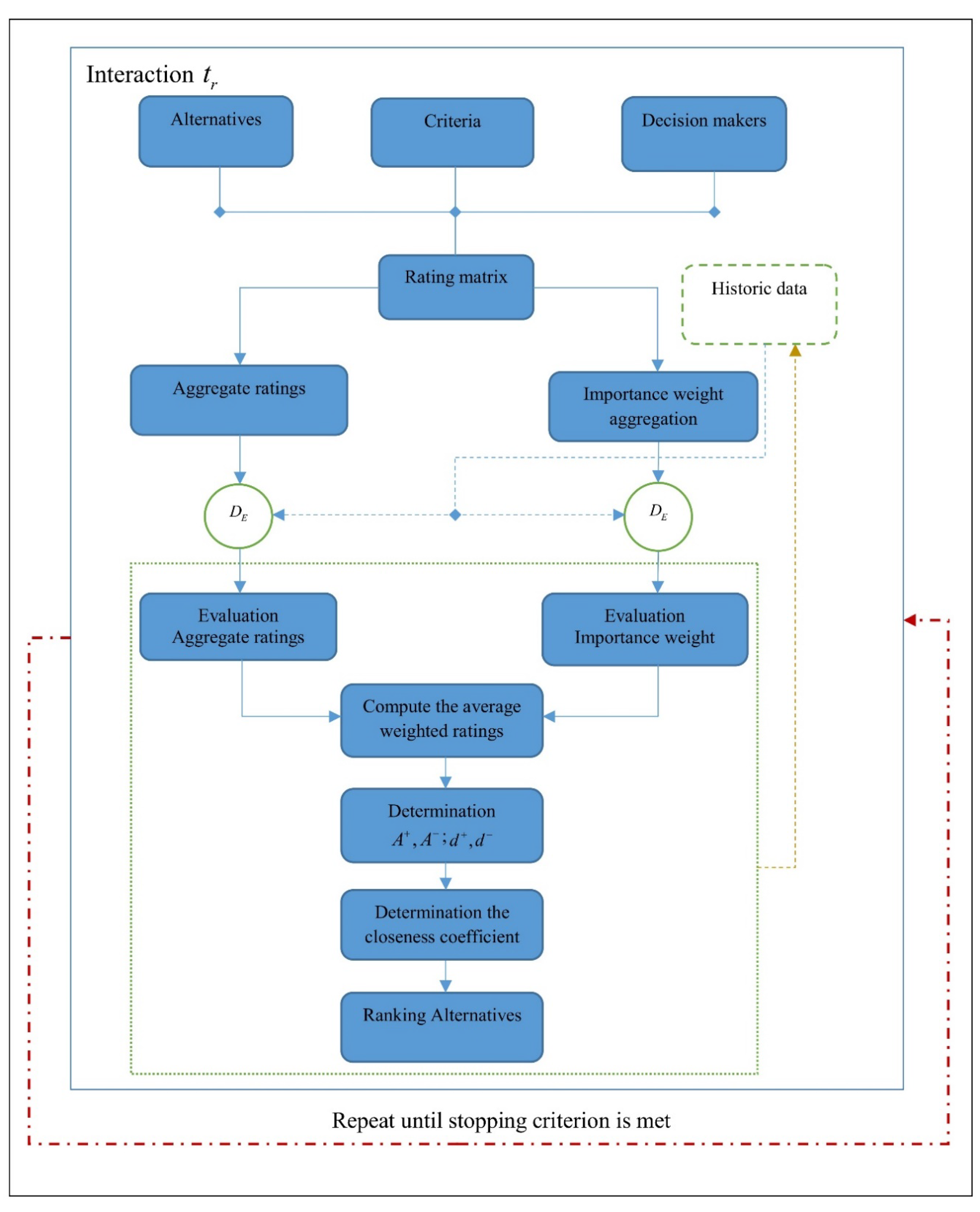
4. Dynamic TOPSIS Method

Based on the theory of GDVINS, the dynamic decision-making model is proposed to deal with the change of criteria, alternatives, and decision-makers during time.

For each period $t=\left\{t_1,t_2,\dots ,t_s\right\}$, assume $\tilde{A}\left(t_r\right)=\left\{A_1,A_2,\dots ,A_{v_r}\right\}$ and $\tilde{C}\left(t_r\right)=\left\{C_1,C_2,\dots ,C_{n_{{}_r}}\right\}$ and $\tilde{D}\left(t_r\right)=\left\{D_1,D_2,\dots ,D_{h_r}\right\}$ being the sets of alternatives, criteria, and decision-makers at period r^th, $r=\left\{1,2,\dots ,s\right\}$. For a decision-maker $D_q;q=1,\dots ,h_r,$ the evaluation of an alternative $A_m;m=1,\dots ,v_r,$ on a criteria $C_p;p=1,\dots ,n_r,$ in time sequence $\tau =\left\{{\tau }_1,{\tau }_2,\dots ,{\tau }_{k_r}\right\}$ is represented by the Neutrosophic decision matrix ${\Re }^q\left(t_r\right)={\left({\xi }_{mp}^q\left(\tau \right)\right)}_{v_r\times n_r};l=1,2,\dots ,k_r.$ where

$${\xi }_{mp}^q\left(\tau \right)=\langle x_{d_{mp}}^q\left(\tau \right),\left(T^q\left(d_{mp},\tau \right),I^q\left(d_{mp},\tau \right),F^q\left(d_{mp},\tau \right)\right)\rangle ;$$

taken by GDIVNSs evaluated by decision maker $D_q$.

Step 1. Calculate aggregate ratings at period r^th.

Let $x_{mpq}\left({\tau }_l\right)=\left\{\left[T_{mpq}^L\left(x_{{\tau }_l}\right),T_{mpq}^U\left(x_{{\tau }_l}\right)\right],\left[I_{mpq}^L\left(x_{{\tau }_l}\right),I_{mpq}^U\left(x_{{\tau }_l}\right)\right],\left[F_{mpq}^L\left(x_{{\tau }_l}\right),F_{mpq}^U\left(x_{{\tau }_l}\right)\right]\right\}$ be the appropriateness rating of alternative $A_m$ for criterion $C_p$ by decision-maker $D_q$ in time sequence ${\tau }_l,$ where: $m=1,\dots ,v_r;p=1,\dots ,n_r;q=1,\dots ,h_r;l=1,\dots ,k_r$. The averaged appropriateness rating $\overline{x_{mp}}=\left\{\left[\overline{T_{mp}^L\left(x\right)},\overline{T_{mp}^U\left(x\right)}\right],\left[\overline{I_{mp}^L\left(x\right)},\overline{I_{mp}^U\left(x\right)}\right],\left[\overline{F_{mp}^L\left(x\right)},\overline{F_{mp}^U\left(x\right)}\right]\right\}$ can be evaluated as:

$$\overline{x_{mp}}=\frac{1}{h_r\times k_r}\times \langle \begin{array}{l}\left[1-{\left\{1-{\left(1-{\displaystyle \sum _{q=1}^{h_r}{T}_{pmq}^L\left(x_{{\tau }_l}\right)}\right)}^{\frac{1}{h_r}}\right\}}^{\frac{1}{k_r}},1-{\left\{1-{\left(1-{\displaystyle \sum _{q=1}^h{T}_{pmq}^U\left(x_{{\tau }_l}\right)}\right)}^{\frac{1}{h_r}}\right\}}^{\frac{1}{k_r}}\right],\\ \left[{\left({\displaystyle \sum _{q=1}^h{I}_{pmq}^L\left(x_{{\tau }_l}\right)}\right)}^{\frac{1}{h_r\times k_r}},{\left({\displaystyle \sum _{q=1}^h{I}_{pmq}^U\left(x_{{\tau }_l}\right)}\right)}^{\frac{1}{h_r\times k_r}}\right],\\ \left[{\left({\displaystyle \sum _{q=1}^h{F}_{pmq}^L\left(x_{{\tau }_l}\right)}\right)}^{\frac{1}{h_r\times k_r}},{\left({\displaystyle \sum _{q=1}^h{F}_{pmq}^U\left(x_{{\tau }_l}\right)}\right)}^{\frac{1}{h_r\times k_r}}\right]\end{array}\rangle$$

(19)

Step 2. Calculate importance weight aggregation at period r^th.

Let $y_{pq}\left({\tau }_l\right)=\left\{\left[T_{pq}^L\left(y_{{\tau }_l}\right),T_{pq}^U\left(y_{{\tau }_l}\right)\right],\left[I_{pq}^L\left(y_{{\tau }_l}\right),I_{pq}^U\left(y_{{\tau }_l}\right)\right],\left[F_{pq}^L\left(y_{{\tau }_l}\right),F_{pq}^U\left(y_{{\tau }_l}\right)\right]\right\}$ be the weight of $D_q$ to criterion $C_p$ in time sequence ${\tau }_l,$ where: $p=1,\dots ,n_r;q=1,\dots ,h_r;l=1,\dots ,k.$ The average weight $\overline{w_p}=\left\{\left[\overline{T_p^L\left(y\right)},\overline{T_p^U\left(y\right)}\right],\left[\overline{I_p^L\left(y\right)},\overline{I_p^U\left(y\right)}\right],\left[\overline{F_p^L\left(y\right)},\overline{F_p^U\left(y\right)}\right]\right\}$ can be evaluated as:

$$\overline{w_p}=\frac{1}{h_r\times k_r}\times \langle \begin{array}{l}\left[1-{\left\{1-{\left(1-{\displaystyle \sum _{q=1}^{h_r}{T}_{pq}^L\left(y_{{\tau }_l}\right)}\right)}^{\frac{1}{h_r}}\right\}}^{\frac{1}{k_r}},1-{\left\{1-{\left(1-{\displaystyle \sum _{q=1}^h{T}_{pq}^U\left(y_{{\tau }_l}\right)}\right)}^{\frac{1}{h_r}}\right\}}^{\frac{1}{k_r}}\right],\\ \left[{\left({\displaystyle \sum _{q=1}^{h_r}{I}_{pq}^L\left(y_{{\tau }_l}\right)}\right)}^{\frac{1}{h_r\times k_r}},{\left({\displaystyle \sum _{q=1}^{h_r}{I}_{pq}^U\left(y_{{\tau }_l}\right)}\right)}^{\frac{1}{h_r\times k_r}}\right],\\ \left[{\left({\displaystyle \sum _{q=1}^{h_r}{F}_{pq}^L\left(y_{{\tau }_l}\right)}\right)}^{\frac{1}{h_r\times k_r}},{\left({\displaystyle \sum _{q=1}^{h_r}{F}_{pq}^U\left(y_{{\tau }_l}\right)}\right)}^{\frac{1}{h_r\times k_r}}\right]\end{array}\rangle ,$$

(20)

Step 3. Evaluation for aggregate ratings of alternatives with history data.

Using Equation (21), evaluate aggregate ratings and importance weight aggregation.

$$\tilde{A}\left(t_r^{*}\right)=\left\{A_1,A_2,\dots ,A_{v_r}\right\}\cup \tilde{A}\left(t_{r-1}\right)$$

$$\overline{x_{mp}^{\ast }}=\{\begin{array}{l}\overline{x_{mp}^r}\begin{array}{ccc}& if& \left(\begin{array}{l}{A}_m\in \tilde{A}\left(t_r\right)\backslash \tilde{A}\left(t_{r-1}\right)\&C_p\in \tilde{C}\left(t_r\right)\backslash \tilde{C}\left(t_{r-1}\right)\\ \begin{array}{cc}or& A_m\in \tilde{A}\left(t_{r-1}\right)\backslash \tilde{A}\left(t_r\right)\&C_p\in \tilde{C}\left(t_r\right)\backslash \tilde{C}\left(t_{r-1}\right)\end{array}\\ \begin{array}{cc}or& A_m\in \tilde{A}\left(t_r\right)\backslash \tilde{A}\left(t_{r-1}\right)\&C_p\in \tilde{C}\left(t_{r-1}\right)\backslash \tilde{C}\left(t_r\right)\end{array}\end{array}\right)\end{array}\\ \overline{x_{mp}^r}\oplus \overline{x_{mp}^{r-1}}\begin{array}{cc}& if\begin{array}{cc}& A_m\in \tilde{A}\left(t_r\right)\cap \tilde{A}\left(t_{r-1}\right)\&C_p\in \tilde{C}\left(t_r\right)\cap \tilde{C}\left(t_{r-1}\right)\end{array}\end{array}\\ \\ \overline{x_{mp}^{r-1}}\begin{array}{ccc}& if& A_m\in \tilde{A}\left(t_{r-1}\right)\backslash \tilde{A}\left(t_r\right)\&C_p\in \tilde{C}\left(t_{r-1}\right)\backslash \tilde{C}\left(t_r\right)\end{array}\end{array}$$

(21)

Step 4. Evaluation for importance weight aggregation of criteria with history data.

Using Equation (22), evaluate aggregate ratings and importance weight aggregation.

$$\tilde{C}\left(t_r^{*}\right)=\left\{C_1,C_2,\dots ,C_{n_{{}_r}}\right\}\cup \tilde{C}\left(t_{r-1}\right)$$

$$\overline{w_p^{\ast }}=\{\begin{array}{lll}\overline{w_p^r}& if& C_p\in \tilde{C}\left(t_r\right)\backslash \tilde{C}\left(t_{r-1}\right)\\ \overline{w_p^r}\oplus \overline{w_p^{r-1}}& if& C_p\in \tilde{C}\left(t_r\right)\cap \tilde{C}\left(t_{r-1}\right)\\ \overline{w_p^{r-1}}& if& C_p\in \tilde{C}\left(t_{r-1}\right)\backslash \tilde{C}\left(t_r\right)\end{array}$$

(22)

Step 5. Calculate the average weighted ratings at period r^th.

The average weighted ratings of alternatives at period $t_r,$ can be calculated by:

$${\mathsf{\Theta }}_m=\frac{1}{n_r^{\ast }}{\displaystyle \sum _{p=1}^{n_r^{\ast }}\overline{x_{{}_{mp}}^{\ast }}*\overline{w_p^{\ast }};m=1,\dots ,v_r^{\ast };p=1,\dots ,n_r^{\ast };}$$

(23)

Step 6. Determination of$A_r^{+},A_r^{-}$and$d_r^{+},d_r^{-}$at period r^th.

Interval-valued neutrosophic positive ideal solution (PIS, $A_r^{+}$) and interval-valued neutrosophic negative ideal solution (NIS, $A_r^{-}$) are:

$$A_r^{+}=\left\{x,\left\{{\left(\left[1,1\right],\left[0,0\right],\left[0,0\right]\right)}_1,{\left(\left[1,1\right],\left[0,0\right],\left[0,0\right]\right)}_2,\dots ,{\left(\left[1,1\right],\left[0,0\right],\left[0,0\right]\right)}_{n_r^{*}}\right\}\right\}$$

(24)

$$A_r^{-}=\left\{x,\left\{{\left(\left[0,0\right],\left[1,1\right],\left[1,1\right]\right)}_1,{\left(\left[0,0\right],\left[1,1\right],\left[1,1\right]\right)}_2,\dots ,{\left(\left[0,0\right],\left[1,1\right],\left[1,1\right]\right)}_{n_r^{*}}\right\}\right\}$$

(25)

The distances of each alternative $A_m,m=1,2,\dots ,n^{*}$ from $A_r^{+}$ and $A_r^{-}$ at period $t_r,$ are calculated as:

$$d_m^{+}=\sqrt{{\left({\mathsf{\Theta }}_m-A_r^{+}\right)}^2}$$

(26)

$$d_m^{-}=\sqrt{{\left({\mathsf{\Theta }}_m-A_r^{-}\right)}^2}$$

(27)

where $d_m^{+}$ and $d_m^{-}$ respectively represent the shortest and farthest distances of $A_m.$

Step 7. Determination the closeness coefficient.

The closeness coefficient at period $t_r,$ is calculated in Equation (28), where an alternative that is close to interval-valued neutrosophic PIS and far from interval-valued neutrosophic NIS, has high value:

$$B{C}_m=\frac{d_m^{-}}{d_m^{+}+d_m^{-}}$$

(28)

Step 8. Rank the alternatives.

The alternatives are ranked by their closeness coefficient values. See Figure 1 for illustration.

5. Applications

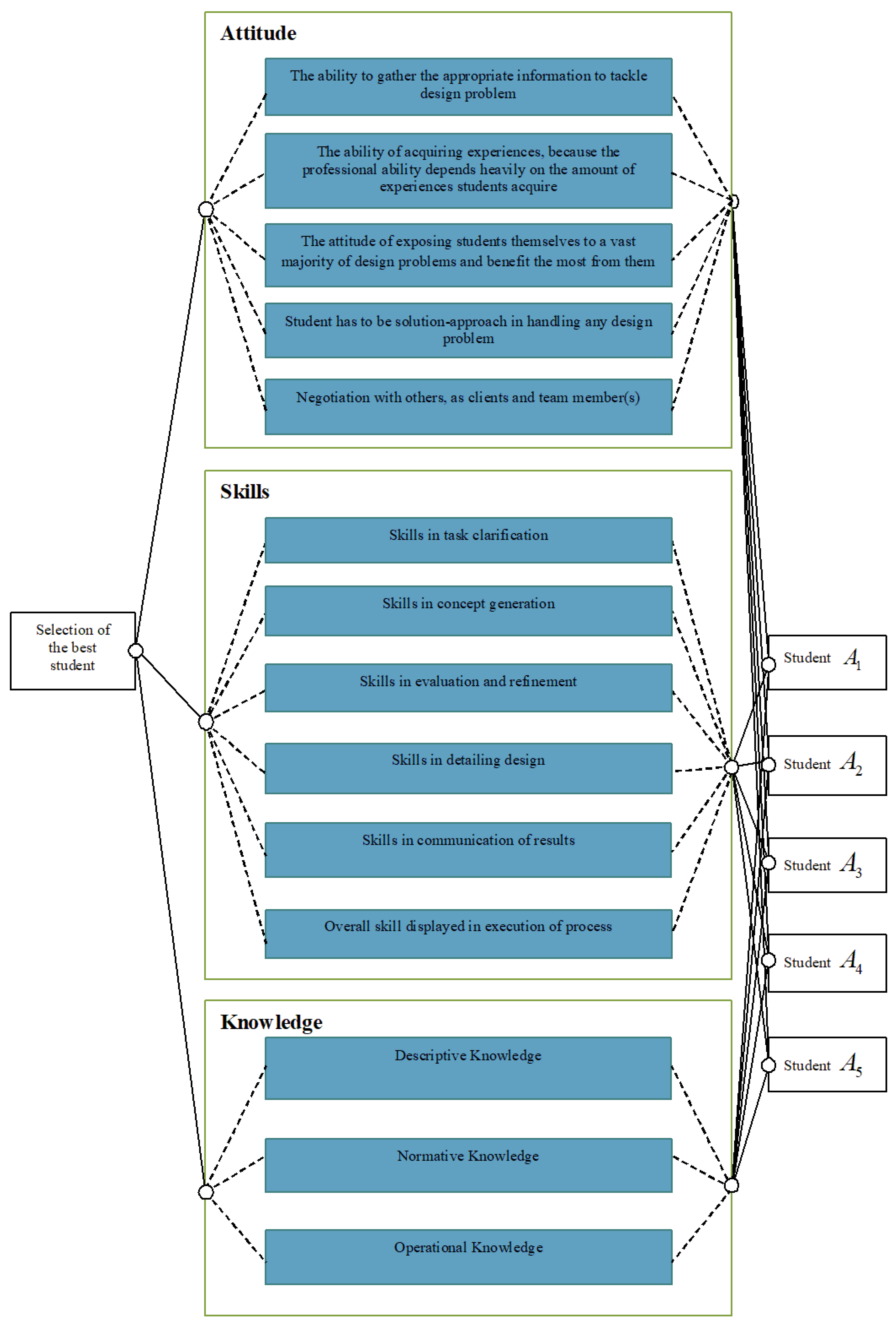
5.1. ASK Model for Ranking Students

Human resources recruitment plays a pivotal role in any enterprise as it exerts tremendous impact on its sustainable development. Thus, the selection of competent and job-relevant staff will lay the solid foundation for the successful performance of an enterprise. Notably, every year most of the businesses invest a large sum of money for job vacancy advertisements (on newspapers, websites, and in job fairs) and recruitment activities including application screening and interview. However, to recruit new graduated student the organizations are likely to encounter high potential risks as there are definitely inevitable employee turnovers or the selected candidates fall short of employers’ expectation [22]. Mis-assessment of candidate’s competence might be rooted from assessors’ criteria and model for new graduated student evaluation.

The above problems underline the need for making the right assessment of potential employees. Currently, ASK model (attitude, skill and knowledge) has been widely used by many organizations because of its comprehensive assessment. This model was initially proposed by Bloom [11] with three factors including knowledge which is acquired through education, comprehension, analysis, and application skills which are the ability to process the knowledge to perform activities or tasks, and attitude which is concerned with feeling, emotions, or motivation toward employment. These elements are given divergent weights in the assessment model according to positions and requirements of the job. ASK is applicable to evaluate tertiary students’ performance to give more information that support employers besides a set of university exit benchmark. It also facilitates students to make proper self-adjustments and pursue appropriate professional orientation for their future career [23,24]. Ranking students based on attributes of ASK model requires a dynamic multi-criteria decision-making model that is able to combine the estimations of different lecturers in different periods. The proposed DTOPSIS completely fit to this complex task, and the application model is depicted bellow.

5.2. Application Model

As mentioned above, the proposed method is applied to rank students of Thuongmai University, Hanoi, Vietnam. In this research, the datasets were surveyed through three consecutive semesters under three criteria (attitudes-skills-knowledge). Each student will be surveyed at the beginning of semester and by the end of semester. With the model assessing student competence, it will be conducted over semesters and over school years. This is the way of setting the time period in the decision-making model of this research.

Figure 2 shows the ASK model for ranking students where three lectures i.e., $D_1,D_2,D_3$ are chosen. According to the language labels shown in

Table 1. Appropriateness ratings.

Language Labels	Values
Very Poor	([0.1, 0.26], [0.4, 0.5], [0.63, 0.76])
Poor	([0.26, 0.38], [0.47, 0.6], [0.51, 0.6])
Medium	([0.38, 0.5], [0.4, 0.61], [0.44, 0.55])
Good	([0.5, 0.65], [0.36, 0.5], [0.31, 0.48])
Very Good	([0.65, 0.8], [0.1, 0.2], [0.12, 0.2])

and

Table 2. The importance of criteria.

Language Labels	Values
Unimportant	([0.1, 0.19], [0.32, 0.47], [0.64, 0.8])
Slightly Important	([0.2, 0.38], [0.46, 0.62], [0.36, 0.55])
Important	([0.45, 0.63], [0.41, 0.53], [0.2, 0.42])
Very Important	([0.66, 0.8], [0.3, 0.39], [0.22, 0.32])
Absolutely Important	([0.8, 0.94], [0.18, 0.29], [0.1, 0.2])

, rating of five students and criteria’ weights are done by the lectures based on fourteenth criteria in three groups: attitude, skill, and knowledge. The attitude group includes five criteria [25], the skill group includes six criteria [26], and the knowledge group includes three criteria [23].

The criteria used for ranking Thuongmai university’s students contain 14 criteria divided into three groups (attitudes-skills-knowledge) in the ASK model. In the early stage of each semester, the knowledge criteria will not cause many impacts on student competency assessment so that we only pay attention to 11 criteria in the two remaining groups: attitudes and skills. In the following semesters, the knowledge criterion shall be supplemented that why all 14 criteria in three group shall be conducted.

(1) Period $t_1$ (the first semester): the decision-maker provides assessments of three students $A_1,A_2,A_3$ according to 11 criteria in two groups: attitude, skill.

Table 3. Aggregated ratings at period $t_1$.

Criteria	Students
	${\mathit{A}}_1$	${\mathit{A}}_2$	${\mathit{A}}_3$
$C_1$	([0.463, 0.606], [0.018, 0.054], [0.014, 0.044])	([0.38, 0.5], [0.022, 0.082], [0.029, 0.059])	([0.43, 0.577], [0.021, 0.053], [0.017, 0.048])
$C_2$	([0.488, 0.632], [0.005, 0.025], [0.008, 0.021])	([0.419,0.578], [0.011,0.037], [0.011,0.026])	([0.419,0.578], [0.011,0.037], [0.011,0.026])
$C_3$	([0.463, 0.606], [0.018, 0.054], [0.014, 0.044])	([0.463, 0.606], [0.018, 0.054], [0.014, 0.044])	([0.423, 0.556], [0.02, 0.066], [0.02, 0.051])
$C_4$	([0.423, 0.556], [0.02, 0.066], [0.02, 0.051])	([0.463, 0.606], [0.018, 0.054], [0.014, 0.044])	([0.388, 0.523], [0.023, 0.065], [0.024, 0.056])
$C_5$	([0.523, 0.673], [0.005, 0.021], [0.005, 0.018])	([0.423, 0.556], [0.02, 0.066], [0.02, 0.051])	([0.43, 0.577], [0.021, 0.053], [0.017, 0.048])
$C_6$	([0.43, 0.577], [0.021, 0.053], [0.017, 0.048])	([0.38, 0.5], [0.022, 0.082], [0.029, 0.059])	([0.342, 0.463], [0.026, 0.081], [0.034, 0.065])
$C_7$	([0.38, 0.5], [0.022, 0.082], [0.029, 0.059])	([0.388, 0.523], [0.023, 0.065], [0.024, 0.056])	([0.342, 0.463], [0.026, 0.081], [0.034, 0.065])
$C_8$	([0.26, 0.38], [0.036, 0.078], [0.046, 0.078])	([0.38, 0.5], [0.022, 0.082], [0.029, 0.059])	([0.38, 0.5], [0.022, 0.082], [0.029, 0.059])
$C_9$	([0.463, 0.606], [0.018, 0.054], [0.014, 0.044])	([0.523, 0.673], [0.005, 0.021], [0.005, 0.018])	([0.463, 0.606], [0.018, 0.054], [0.014, 0.044])
$C_{10}$	([0.5, 0.65], [0.016, 0.044], [0.01, 0.038])	([0.38, 0.5], [0.022, 0.082], [0.029, 0.059])	([0.43, 0.577], [0.021, 0.053], [0.017, 0.048])
$C_{11}$	([0.463, 0.606], [0.018, 0.054], [0.014, 0.044])	([0.302, 0.423], [0.03, 0.079], [0.04, 0.071])	([0.38, 0.5], [0.022, 0.082], [0.029, 0.059])

and

Table 4. Aggregated weights at period $t_1$.

Criteria	Importance Aggregated Weights
$C_1$	([0.963, 0.996], [0.022, 0.06], [0.004, 0.027])
$C_2$	([0.908, 0.968], [0.041, 0.094], [0.017, 0.056])
$C_3$	([0.758, 0.89], [0.077, 0.174], [0.014, 0.097])
$C_4$	([0.648, 0.816], [0.087, 0.204], [0.026, 0.127])
$C_5$	([0.604, 0.794], [0.06, 0.154], [0.046, 0.185])
$C_6$	([0.963, 0.992], [0.022, 0.06], [0.004, 0.027])
$C_7$	([0.834, 0.925], [0.069, 0.149], [0.008, 0.074])
$C_8$	([0.758, 0.89], [0.077, 0.174], [0.014, 0.097])
$C_9$	([0.758, 0.89], [0.077, 0.174], [0.014, 0.097])
$C_{10}$	([0.936, 0.975], [0.037, 0.081], [0.01, 0.043])
$C_{11}$	([0.897, 0.959], [0.05, 0.11], [0.009, 0.056])

show the steps of the model at time $t_1$ and

Table 5. Weighted ratings at period $t_1$.

Students	Weighted Ratings
$A_1$	([0.368, 0.409], [0.069, 0.168], [0.03, 0.114])
$A_2$	([0.34, 0.382], [0.071, 0.181], [0.035, 0.12])
$A_3$	([0.338, 0.377], [0.072, 0.178], [0.035, 0.121])

shows the ranking order as $A_1\succ A_2\succ A_3$. Thus, the best student is $A_1$.

(2) Period $t_2$ (the second semester): At this stage, a new student $A_4$ is added with new criteria in knowledge group. The steps are shown in

Table 6. The distance of each student from $A_{t_1}^{+}$ and $A_{t_1}^{-}$ at period $t_1$.

Students	${\mathit{d}}_{{\mathit{t}}_1}^{+}$	${\mathit{d}}_{{\mathit{t}}_1}^{-}$
$A_1$	0.364193	0.773329
$A_2$	0.380989	0.763987
$A_3$	0.382736	0.763579

,

Table 7. Closeness coefficient at period $t_1$.

Students	Closeness Coefficients	Ranking Order
$A_1$	0.679837	1
$A_2$	0.667251	2
$A_3$	0.666116	3

,

Table 8. Aggregated ratings at period $t_2$.

Criteria	Students
	${\mathit{A}}_1$	${\mathit{A}}_2$	${\mathit{A}}_3$	${\mathit{A}}_4$
$C_1$	([0.699, 0.83], [0.001, 0.005], [0, 0.002])	([0.566, 0.75], [0.001, 0.009], [0.001, 0.003])	([0.637, 0.759], [0.001, 0.007], [0.001, 0.003])	([0.5, 0.6], [0.022, 0.046], [0.009, 0.022])
$C_2$	([0.707, 0.852], [0.001, 0.007], [0, 0.002])	([0.686, 0.834], [0.001, 0.008], [0, 0.003])	([0.72, 0.862], [0.001, 0.006], [0, 0.002])	([0.498, 0.6], [0.023, 0.049], [0.009, 0.023])
$C_3$	([0.709, 0.848], [0.003, 0.016], [0, 0.005])	([0.643, 0.783], [0.003, 0.018], [0, 0.006])	([0.603, 0.767], [0.003, 0.019], [0.001, 0.006])	([0.56, 0.669], [0.008, 0.029], [0.004, 0.016])
$C_4$	([0.598, 0.766], [0.004, 0.022], [0.001, 0.007])	([0.639, 0.782], [0.004, 0.021], [0.001, 0.007])	([0.634, 0.793], [0.004, 0.02], [0.001, 0.008])	([0.506, 0.643], [0.009, 0.034], [0.006, 0.021])
$C_5$	([0.721, 0.866], [0.002, 0.012], [0.001, 0.015])	([0.651, 0.823], [0.002, 0.013], [0.002, 0.016])	([0.616, 0.765], [0.002, 0.014], [0.002, 0.017])	([0.461, 0.604], [0.013, 0.042], [0.009, 0.035])
$C_6$	([0.685, 0.81], [0.001, 0.005], [0, 0.002])	([0.623, 0.803], [0.001, 0.007], [0, 0.002])	([0.546, 0.72], [0.001, 0.009], [0.001, 0.004])	([0.3, 0.5], [0.022, 0.08], [0.022, 0.044])
$C_7$	([0.62, 0.802], [0.002, 0.013], [0, 0.004])	([0.618, 0.769], [0.002, 0.013], [0.001, 0.005])	([0.543, 0.72], [0.002, 0.015], [0.001, 0.006])	([0.438, 0.569], [0.024, 0.061], [0.012, 0.03])
$C_8$	([0.491, 0.648], [0.005, 0.025], [0.002, 0.013])	([0.686, 0.862], [0.004, 0.02], [0, 0.006])	([0.499, 0.709], [0.005, 0.025], [0.001, 0.009])	([0.43, 0.567], [0.026, 0.071], [0.012, 0.033])
$C_9$	([0.702, 0.847], [0.004, 0.021], [0, 0.007])	([0.761, 0.891], [0.004, 0.019], [0, 0.006])	([0.682, 0.828], [0.004, 0.022], [0, 0.007])	([0.488, 0.598], [0.026, 0.062], [0.009, 0.027])
$C_{10}$	([0.687, 0.8], [0.002, 0.01], [0, 0.003])	([0.663, 0.836], [0.001, 0.008], [0, 0.003])	([0.718, 0.842], [0.001, 0.008], [0, 0.003])	([0.534, 0.636], [0.012, 0.032], [0.006, 0.018])
$C_{11}$	([0.608, 0.751], [0.001, 0.009], [0.001, 0.003])	([0.557, 0.722], [0.001, 0.01], [0.001, 0.006])	([0.565, 0.75], [0.001, 0.011], [0.001, 0.004])	([0.499, 0.6], [0.023, 0.048], [0.009, 0.023])
$C_{12}$	([0.36, 0.533], [0.043, 0.12], [0.021, 0.06])	([0.4, 0.516], [0.049, 0.11], [0.023, 0.065])	([0.463, 0.606], [0.033, 0.089], [0.012, 0.047])	([0.258, 0.439], [0.049, 0.133], [0.037, 0.087])
$C_{13}$	([0.229, 0.373], [0.05, 0.119], [0.055, 0.108])	([0.229, 0.373], [0.05, 0.119], [0.055, 0.108])	([0.43, 0.568], [0.038, 0.095], [0.017, 0.047])	([0.43, 0.568], [0.038, 0.095], [0.017, 0.047])
$C_{14}$	([0.284, 0.408], [0.083, 0.167], [0.046, 0.123])	([0.284, 0.408], [0.083, 0.167], [0.046, 0.123])	([0.269, 0.486], [0.071, 0.179], [0.03, 0.098])	([0.431, 0.592], [0.061, 0.137], [0.017, 0.076])

,

Table 9. Aggregated weights at period $t_2$.

Criteria	Importance Aggregated Weights
$C_1$	([0.999, 1], [0, 0.003], [0, 0.001])
$C_2$	([0.997, 1], [0.001, 0.006], [0, 0.002])
$C_3$	([0.985, 0.998], [0.003, 0.014], [0, 0.004])
$C_4$	([0.978, 0.997], [0.003, 0.016], [0, 0.005])
$C_5$	([0.959, 0.993], [0.002, 0.011], [0.001, 0.015])
$C_6$	([0.999, 1], [0, 0.003], [0, 0.001])
$C_7$	([0.993, 0.999], [0.002, 0.009], [0, 0.002])
$C_8$	([0.975, 0.997], [0.004, 0.019], [0, 0.005])
$C_9$	([0.975, 0.997], [0.004, 0.019], [0, 0.005])
$C_{10}$	([0.996, 1], [0.001, 0.006], [0, 0.002])
$C_{11}$	([0.998, 1], [0.001, 0.005], [0, 0.001])
$C_{12}$	([0.963, 0.996], [0.022, 0.06], [0.004, 0.027])
$C_{13}$	([0.977, 0.998], [0.016, 0.044], [0.005, 0.02])
$C_{14}$	([0.897, 0.973], [0.05, 0.11], [0.009, 0.056])

,

Table 10. Weighted ratings at period $t_2$.

Students	Weighted Ratings
$A_1$	([0.605, 0.76], [0.004, 0.02], [0.001, 0.009])
$A_2$	([0.594, 0.761], [0.004, 0.02], [0.001, 0.009])
$A_3$	([0.581, 0.744], [0.004, 0.021], [0.001, 0.009])
$A_4$	([0.458, 0.588], [0.022, 0.058], [0.011, 0.031])

,

Table 11. The distance of each student from $A_{t_2}^{+}$ and $A_{t_2}^{-}$ at period $t_2$.

Students	${\mathit{d}}_{{\mathit{t}}_2}^{+}$	${\mathit{d}}_{{\mathit{t}}_2}^{-}$
$A_1$	0.188874	0.901553
$A_2$	0.192392	0.900405
$A_3$	0.200641	0.896588
$A_4$	0.279475	0.848118

and

Table 12. Closeness coefficient at period $t_2$.

Students	Closeness Coefficients	Ranking Order
$A_1$	0.826789	1
$A_2$	0.823945	2
$A_3$	0.817138	3
$A_4$	0.752149	4

. Finally, the ranking is obtained: $A_1\succ A_2\succ A_3\succ A_4$. Thus, the best student is $A_1$.

(3) Period $t_3$ (the third semester): At this stage, a new student $A_5$ is considered and an existing student $A_2$ is discarded. The criteria remain the same as in the previous period $t_2$.

Table 13. Aggregated ratings at period $t_3$.

Criteria	Students
	${\mathit{A}}_1$	${\mathit{A}}_2$	${\mathit{A}}_3$	${\mathit{A}}_4$	${\mathit{A}}_5$
$C_1$	([0.794, 0.9], [0, 0], [0, 0])	([0.51, 0.75], [0, 0.006], [0, 0.002])	([0.764, 0.893], [0, 0], [0, 0])	([0.711, 0.822], [0, 0.003], [0, 0.001])	([0.441, 0.569], [0.022, 0.053], [0.012, 0.027])
$C_2$	([0.871, 0.951], [0, 0], [0, 0])	([0.675, 0.818], [0, 0.002], [0, 0.001])	([0.881, 0.96], [0, 0], [0, 0])	([0.788, 0.891], [0, 0.001], [0, 0])	([0.441, 0.569], [0.022, 0.053], [0.012, 0.027])
$C_3$	([0.829, 0.918], [0, 0.001], [0, 0])	([0.608, 0.785], [0.001, 0.005], [0, 0.001])	([0.728, 0.884], [0, 0.001], [0, 0])	([0.817, 0.91], [0, 0.001], [0, 0])	([0.569, 0.67], [0.005, 0.016], [0.004, 0.012])
$C_4$	([0.711, 0.875], [0, 0.001], [0, 0])	([0.608, 0.785], [0.001, 0.005], [0, 0.001])	([0.816, 0.922], [0, 0.001], [0, 0])	([0.663, 0.795], [0, 0.002], [0, 0.001])	([0.569, 0.67], [0.005, 0.016], [0.004, 0.012])
$C_5$	([0.81, 0.912], [0, 0.001], [0, 0.001])	([0.635, 0.804], [0, 0.003], [0, 0.001])	([0.777, 0.889], [0, 0.001], [0, 0.001])	([0.751, 0.872], [0, 0.001], [0, 0.001])	([0.48, 0.608], [0.011, 0.032], [0.008, 0.021])
$C_6$	([0.832, 0.923], [0, 0], [0, 0])	([0.608, 0.785], [0, 0.004], [0, 0.001])	([0.744, 0.902], [0, 0], [0, 0])	([0.482, 0.69], [0.001, 0.006], [0.001, 0.003])	([0.536, 0.637], [0.011, 0.026], [0.006, 0.016])
$C_7$	([0.689, 0.86], [0, 0.001], [0, 0])	([0.591, 0.759], [0.001, 0.004], [0, 0.002])	([0.682, 0.86], [0, 0.001], [0, 0])	([0.586, 0.733], [0.001, 0.004], [0.001, 0.002])	([0.441, 0.569], [0.022, 0.053], [0.012, 0.027])
$C_8$	([0.751, 0.898], [0, 0.001], [0, 0])	([0.662, 0.822], [0, 0.003], [0, 0.001])	([0.732, 0.89], [0, 0.001], [0, 0])	([0.699, 0.83], [0, 0.004], [0, 0.001])	([0.268, 0.441], [0.027, 0.079], [0.033, 0.062])
$C_9$	([0.874, 0.95], [0, 0.002], [0, 0])	([0.749, 0.861], [0, 0.002], [0, 0.001])	([0.889, 0.963], [0, 0.002], [0, 0])	([0.743, 0.853], [0, 0.003], [0, 0.001])	([0.418, 0.578], [0.011, 0.039], [0.011, 0.026])
$C_{10}$	([0.757, 0.891], [0, 0], [0, 0])	([0.636, 0.804], [0, 0.003], [0, 0.001])	([0.837, 0.926], [0, 0], [0, 0])	([0.712, 0.818], [0, 0.002], [0, 0.001])	([0.5, 0.6], [0.022, 0.044], [0.009, 0.022])
$C_{11}$	([0.753, 0.88], [0, 0], [0, 0])	([0.521, 0.71], [0.001, 0.005], [0.001, 0.003])	([0.696, 0.875], [0, 0.001], [0, 0])	([0.651, 0.769], [0.001, 0.004], [0, 0.002])	([0.569, 0.67], [0.005, 0.015], [0.004, 0.012])
$C_{12}$	([0.753, 0.884], [0.001, 0.007], [0, 0.002])	([0.53, 0.662], [0.002, 0.011], [0.001, 0.007])	([0.778, 0.903], [0.001, 0.007], [0, 0.002])	([0.544, 0.72], [0.002, 0.013], [0.001, 0.005])	([0.534, 0.636], [0.012, 0.032], [0.006, 0.018])
$C_{13}$	([0.677, 0.845], [0, 0.002], [0, 0.001])	([0.338, 0.521], [0.001, 0.006], [0.003, 0.009])	([0.759, 0.881], [0, 0.002], [0, 0])	([0.699, 0.83], [0.001, 0.004], [0, 0.001])	([0.374, 0.536], [0.022, 0.065], [0.016, 0.035])
$C_{14}$	([0.688, 0.837], [0.001, 0.005], [0, 0.001])	([0.407, 0.555], [0.002, 0.008], [0.002, 0.008])	([0.777, 0.916], [0.001, 0.005], [0, 0.001])	([0.699, 0.826], [0.001, 0.007], [0, 0.002])	([0.44, 0.569], [0.023, 0.057], [0.012, 0.029])

,

Table 14. Aggregated weights at period $t_3$.

Criteria	Importance Aggregated Weights
$C_1$	([0.99999, 1], [0, 0.00009], [0, 0.00001])
$C_2$	([0.99995, 1], [0.00001, 0.00019], [0, 0.00002])
$C_3$	([0.99964, 1], [0.00005, 0.00062], [0, 0.00009])
$C_4$	([0.99912, 0.99998], [0.00009, 0.00097], [0, 0.00018])
$C_5$	([0.99776, 0.99995], [0.00004, 0.00077], [0.00001, 0.00053])
$C_6$	([0.99999, 1], [0, 0.00006], [0, 0])
$C_7$	([0.99985, 1], [0.00003, 0.00039], [0, 0.00005])
$C_8$	([0.99907, 0.99999], [0.00009, 0.00114], [0, 0.00015])
$C_9$	([0.99842, 0.99996], [0.00014, 0.00154], [0, 0.00024])
$C_{10}$	([0.99991, 1], [0.00002, 0.00029], [0, 0.00004])
$C_{11}$	([0.99997, 1], [0.00001, 0.00016], [0, 0.00001])
$C_{12}$	([0.99615, 0.99988], [0.00112, 0.00657], [0.00004, 0.00152])
$C_{13}$	([0.99969, 1], [0.00016, 0.00145], [0.00001, 0.00026])
$C_{14}$	([0.99762, 0.99993], [0.00082, 0.00483], [0.00004, 0.00116])

,

Table 15. Weighted ratings at period $t_3$.

Students	Weighted Ratings
$A_1$	([0.78, 0.901], [0, 0.001], [0, 0])
$A_2$	([0.589, 0.759], [0.001, 0.004], [0, 0.002])
$A_3$	([0.785, 0.91], [0, 0.001], [0, 0])
$A_4$	([0.693, 0.822], [0, 0.003], [0, 0.001])
$A_5$	([0.476, 0.599], [0.014, 0.037], [0.009, 0.022])

,

Table 16. The distance of each student from $A_{t_3}^{+}$ and $A_{t_3}^{-}$ at period $t_3$.

Students	${\mathit{d}}_{{\mathit{t}}_3}^{+}$	${\mathit{d}}_{{\mathit{t}}_3}^{-}$
$A_1$	0.37844	0.776416
$A_2$	0.352522	0.752181
$A_3$	0.381797	0.777005
$A_4$	0.358066	0.764391
$A_5$	0.325366	0.738391

and

Table 17. Closeness coefficient at period $t_3$.

Students	Closeness Coefficients	Ranking Order
$A_1$	0.672305	4
$A_2$	0.680890	3
$A_3$	0.670525	5
$A_4$	0.680998	2
$A_5$	0.694135	1

show the steps of this stage. Finally, the ranking is obtained: $A_5\succ A_4\succ A_2\succ A_1\succ A_3$. Thus, the best student is $A_5$.

5.3. Comparison with the Related Methods

The proposed dynamic TOPSIS method has superior features compared to the method in [14]. In

Table 18. The dynamic rankings obtained at periods.

Time Period	The Method in [14]	The Proposed Method
$t_1$	$A_1\succ A_2\succ A_3$	$A_1\succ A_2\succ A_3$
$t_2$	$A_4\succ A_2\succ A_3\succ A_1$	$A_1\succ A_2\succ A_3\succ A_4$
$t_3$	$A_5\succ A_3\succ A_4\succ A_1$	$A_5\succ A_4\succ A_2\succ A_1\succ A_3$

, the ranking order of five students in three periods are presented. We can observe that at period $t_1$, the results of the both methods are the same i.e., $A_1\succ A_2\succ A_3$.

At period $t_2$, the method in [14] and the proposed method show difference in ranking order of $A_1$ and $A_4$. In this period, $A_2\succ A_3$ according to both methods, and the method in [14] ranks $A_4$ at the top, meanwhile, $A_1$ is ranked at the top by the proposed method. The reason is that $A_4$ is evaluated at the first time and it has not appeared while $A_1$ has historical data, particularly $A_1$ were ranked at the top in the previous period. In this circumstance, the proposed model better utilizes the effect of historical data on the alternatives $A_1$ and $A_4$. The result of the dynamic TOPSIS model is time-dependent and combines the effect of current and historical data.

At period $t_3$, the result shows difference in the number of ranked alternatives and in their preferential order. In this period, the alternative $A_2$ is not evaluated by decision-makers and it has only historical data. The method in [14] could not process alternative $A_2$, meanwhile the proposed model could. Moreover, the alternative $A_5$ is highly ranked by both methods. However, there is a change in the relative order of $A_3$ and $A_4$. The method in [14] ranks $A_3\succ A_4$, but the proposed method ranks $A_4\succ A_3$.

The comparison between the methods again illustrates the effect of historical data over the output of the proposed decision-making model. If an alternative is considered and it has good evaluation in the previous periods, this alternative will have high potential to reach high order. From that point of view, the proposed model presents good compliance with the perceived dynamic rules. It illustrates the advantage and applicability of the model.

6. Conclusions

The proposed dynamic TOPSIS (DTOPSIS) model in dynamic interval-valued neutrosophic sets presents its advantages to cope with dynamic and indeterminate information in decision-making model. DTOPSIS model handles historical data including the change of criteria, alternatives, and decision-makers during periods. The concepts of generalized dynamic interval-valued neutrosophic set, GDIVNS, and their mathematical operators on GDIVNSs have been proposed. Distance and weighted aggregation operators are used to construct a framework of DTOPSIS in DIVNS environment. The proposed DTOPSIS fulfills the requirement of an issue that is evaluates tertiary students’ performance based on the attributes of ASK model. Data of Thuongmai University students were used to illustrate the proper of DTOPSIS model which opened the potential application in larger scale also. For the future works, we will extend generalized dynamic interval-valued neutrosophic sets for some other real-world applications [27,28,29,30,31,32,33,34,35]. Furthermore, we hope to apply GDIVNS for dealing with the unlimited time problems in decision-making model in dynamic neutrosophic environment based on the idea in [36,37].

References

1. Campanella, G.; Ribeiro, R.A. A framework for dynamic multiple-criteria decision making. Decis. Support Syst. 2011, 52, 52–60. [Google Scholar] [CrossRef]
2. Smarandache, F. Neutrosophy: Neutrosophic Probability, Set, and Logic: Analytic Synthesis & Synthetic Analysis; American Research Press: Santa Fe, NM, USA, 1998. [Google Scholar]
3. Abdel-Basset, M.; Manogaran, G.; Gamal, A.; Smarandache, F. A hybrid approach of neutrosophic sets and DEMATEL method for developing supplier selection criteria. Des. Autom. Embed. Syst. 2018, 22, 257–278. [Google Scholar] [CrossRef] [Green Version]
4. Deli, I.; Broumi, S.; Smarandache, F. On neutrosophic refined sets and their applications in medical diagnosis. J. New Theory 2015, 6, 88–98. [Google Scholar]
5. Peng, J.-J.; Wang, J.-Q.; Wang, J.; Zhang, H.-Y.; Chen, X.-H. Simplified neutrosophic sets and their applications in multi-criteria group decision-making problems. Int. J. Syst. Sci. 2015, 47, 1–17. [Google Scholar] [CrossRef]
6. Şahin, R.; Liu, P. Possibility-induced simplified neutrosophic aggregation operators and their application to multi-criteria group decision-making. J. Exp. Theor. Artif. Intell. 2016, 29, 1–17. [Google Scholar] [CrossRef]
7. Ye, J. Multicriteria decision-making method using the correlation coefficient under single-valued neutrosophic environment. Int. J. Gen. Syst. 2013, 42, 386–394. [Google Scholar] [CrossRef]
8. Ye, J. Single-Valued Neutrosophic Minimum Spanning Tree and Its Clustering Method. J. Intell. Syst. 2014, 23, 311–324. [Google Scholar] [CrossRef] [Green Version]
9. Ye, J. Similarity measures between interval neutrosophic sets and their applications in multicriteria decision-making. J. Intell. Fuzzy Syst. 2014, 26, 165–172. [Google Scholar] [CrossRef]
10. Ye, J. Hesitant interval neutrosophic linguistic set and its application in multiple attribute decision making. Int. J. Mach. Learn. Cybern. 2017, 10, 667–678. [Google Scholar] [CrossRef]
11. Bloom, B.S.; Davis, A.; Hess, R.O.B.E.R.T. Com-Pensatory Education for Cultural Depri-Vation; Holt, Rinehart, &Winston: New York, NY, USA, 1965. [Google Scholar]
12. Huang, Y.-H.; Wei, G.; Wei, C. VIKOR Method for Interval Neutrosophic Multiple Attribute Group Decision-Making. Information 2017, 8, 144. [Google Scholar] [CrossRef] [Green Version]
13. Liu, P.; Shi, L. The generalized hybrid weighted average operator based on interval neutrosophic hesitant set and its application to multiple attribute decision making. Neural Comput. Appl. 2014, 26, 457–471. [Google Scholar] [CrossRef]
14. Thong, N.T.; Dat, L.Q.; Son, L.H.; Hoa, N.D.; Ali, M.; Smarandache, F. Dynamic interval valued neutrosophic set: Modeling decision making in dynamic environments. Comput. Ind. 2019, 108, 45–52. [Google Scholar] [CrossRef]
15. Wang, L.; Zhang, H.-Y.; Wang, J.-Q. Frank Choquet Bonferroni Mean Operators of Bipolar Neutrosophic Sets and Their Application to Multi-criteria Decision-Making Problems. Int. J. Fuzzy Syst. 2017, 20, 13–28. [Google Scholar] [CrossRef]
16. Wang, H.; Smarandache, F.; Sunderraman, R.; Zhang, Y.Q. Interval Neutrosophic Sets and Logic: Theory and Applications in Computing: Theory and Applications in Computing; Infinite Study; Hexis: Phoenix, AZ, USA, 2005; Volume 5. [Google Scholar]
17. Lupiáñez, F.G. Interval neutrosophic sets and topology. Kybernetes 2009, 38, 621–624. [Google Scholar] [CrossRef] [Green Version]
18. Bera, T.; Mahapatra, N.K. Distance Measure Based MADM Strategy with Interval Trapezoidal Neutrosophic Numbers. Neutrosophic Sets Syst. 2018, 20, 7. [Google Scholar]
19. Torra, V.; Narukawa, Y. On hesitant fuzzy sets and decision. In Proceedings of the 2009 IEEE International Conference on Fuzzy Systems, Jeju Island, Korea, 20–24 August 2009; Institute of Electrical and Electronics Engineers (IEEE); pp. 1378–1382. [Google Scholar]
20. Torra, V. Hesitant fuzzy sets. Int. J. Intell. Syst. 2010, 25, 529–539. [Google Scholar] [CrossRef]
21. Rubb, S. Overeducation, undereducation and asymmetric information in occupational mobility. Appl. Econ. 2013, 45, 741–751. [Google Scholar] [CrossRef]
22. Bakarman, A.A. Attitude, Skill, and Knowledge: (ASK) a New Model for Design Education. In Proceedings of the Canadian Engineering Education Association (CEEA), Queen’s University Library, Kingston, ON, Canada, 6–8 June 2011. [Google Scholar]
23. Bell, R. Unpacking the link between entrepreneurialism and employability. Educ. Train. 2016, 58, 2–17. [Google Scholar] [CrossRef]
24. Cross, N. Expertise in design: An overview. Des. Stud. 2004, 25, 427–441. [Google Scholar] [CrossRef] [Green Version]
25. Lewis, W.; Bonollo, E. An analysis of professional skills in design: Implications for education and research. Des. Stud. 2002, 23, 385–406. [Google Scholar] [CrossRef]
26. Son, N.T.K.; Dong, N.P.; Long, H.V.; Son, L.H.; Khastan, A. Linear quadratic regulator problem governed by granular neutrosophic fractional differential equations. ISA Trans. 2020, 97, 296–316. [Google Scholar] [CrossRef] [PubMed]
27. Thong, N.T.; Giap, C.N.; Tuan, T.M.; Chuan, P.M.; Hoang, P.M. Modeling multi-criteria decision-making in dynamic neutrosophic environments bases on Choquet integral. J. Comput. Sci. Cybern. 2020, 36, 33–47. [Google Scholar] [CrossRef]
28. Son, N.T.K.; Dong, N.P.; Son, L.H.; Long, H.V. Towards granular calculus of single-valued neutrosophic functions under granular computing. Multimedia Tools Appl. 2019, 78, 1–37. [Google Scholar] [CrossRef] [Green Version]
29. Son, N.T.K.; Dong, N.P.; Son, L.H.; Abdel-Basset, M.; Manogaran, G.; Long, H.V. On the Stabilizability for a Class of Linear Time-Invariant Systems under Uncertainty. Circuits, Syst. Signal Process. 2019, 39, 919–960. [Google Scholar] [CrossRef]
30. Long, H.V.; Ali, M.; Son, L.H.; Khan, M.; Tu, D.N. A novel approach for fuzzy clustering based on neutrosophic association matrix. Comput. Ind. Eng. 2019, 127, 687–697. [Google Scholar] [CrossRef] [Green Version]
31. Jha, S.; Kumar, R.; Son, L.H.; Chatterjee, J.M.; Khari, M.; Yadav, N.; Smarandache, F. Neutrosophic soft set decision making for stock trending analysis. Evol. Syst. 2018, 10, 621–627. [Google Scholar] [CrossRef] [Green Version]
32. Ngan, R.T.; Son, L.H.; Cuong, B.C.; Ali, M. H-max distance measure of intuitionistic fuzzy sets in decision making. Appl. Soft Comput. 2018, 69, 393–425. [Google Scholar] [CrossRef]
33. Ali, M.; Dat, L.Q.; Son, L.H.; Smarandache, F. Interval Complex Neutrosophic Set: Formulation and Applications in Decision-Making. Int. J. Fuzzy Syst. 2017, 20, 986–999. [Google Scholar] [CrossRef]
34. Nguyen, G.N.; Son, L.H.; Ashour, A.S.; Dey, N. A survey of the state-of-the-arts on neutrosophic sets in biomedical diagnoses. Int. J. Mach. Learn. Cybern. 2017, 10, 1–13. [Google Scholar] [CrossRef] [Green Version]
35. Thong, N.T.; Lan, L.T.H.; Chou, S.-Y.; Son, L.H.; Dong, D.D.; Ngan, T.T. An Extended TOPSIS Method with Unknown Weight Information in Dynamic Neutrosophic Environment. Mathematics 2020, 8, 401. [Google Scholar] [CrossRef] [Green Version]
36. Ali, M.; Son, L.H.; Deli, I.; Tien, N.D. Bipolar neutrosophic soft sets and applications in decision making. J. Intell. Fuzzy Syst. 2017, 33, 4077–4087. [Google Scholar] [CrossRef] [Green Version]
37. Alcantud, J.C.R.; Torrecillas, M.M. Intertemporal Choice of Fuzzy Soft Sets. Symmetry 2018, 10, 371. [Google Scholar] [CrossRef] [Green Version]
Figure 1. Dynamic TOPSIS method.
Symmetry 12 00618 g001
Figure 2. Attitudes-skills-knowledge (ASK) model for recruitment of ternary students.
Symmetry 12 00618 g002