A Monte Carlo Approach to Estimate the Stability of Soil–Rock Slopes Considering the Non-Uniformity of Materials


Abstract
1. Introduction
2. The Monte Carlo Method for Soil–Rock Slopes
2.1. Generation of Independent Random Variables
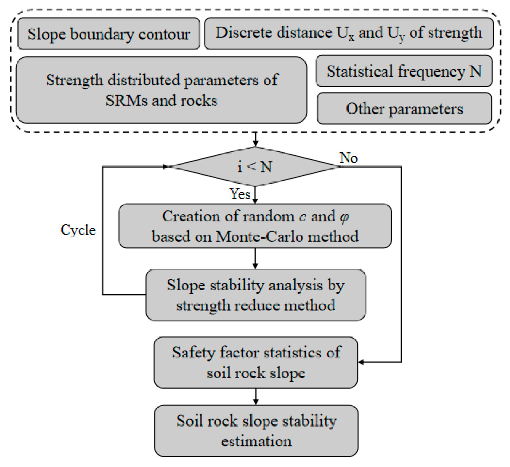
2.2. Stability Analysis of the Soil–Rock Slope by the Monte Carlo Method
2.2.1. Stability Analysis Process for the Soil–Rock Slope
2.2.2. Analysis Model of the Soil–Rock Slope
3. Strength Measurement of Soil–Rock Mixtures
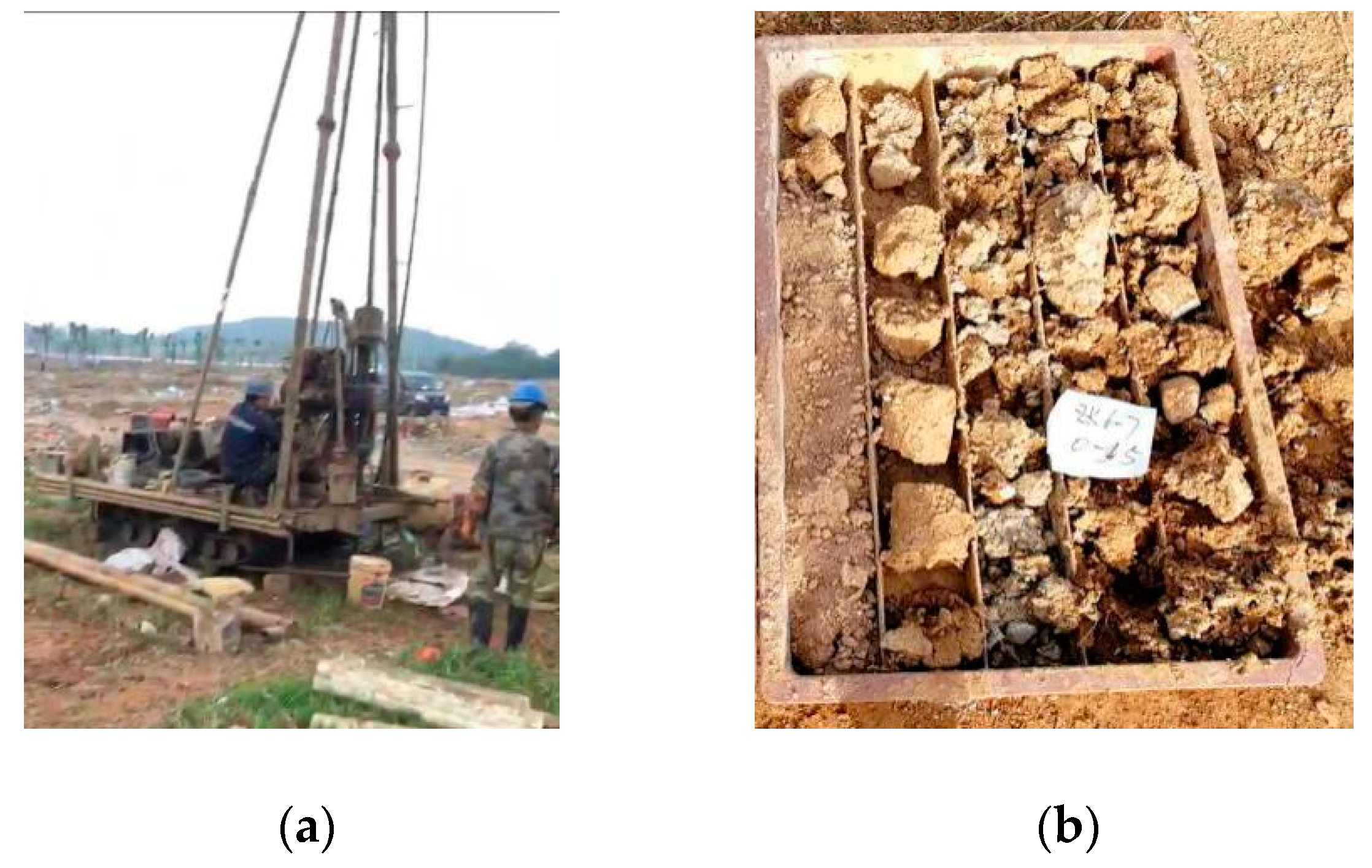
3.1. Acquisition of Samples
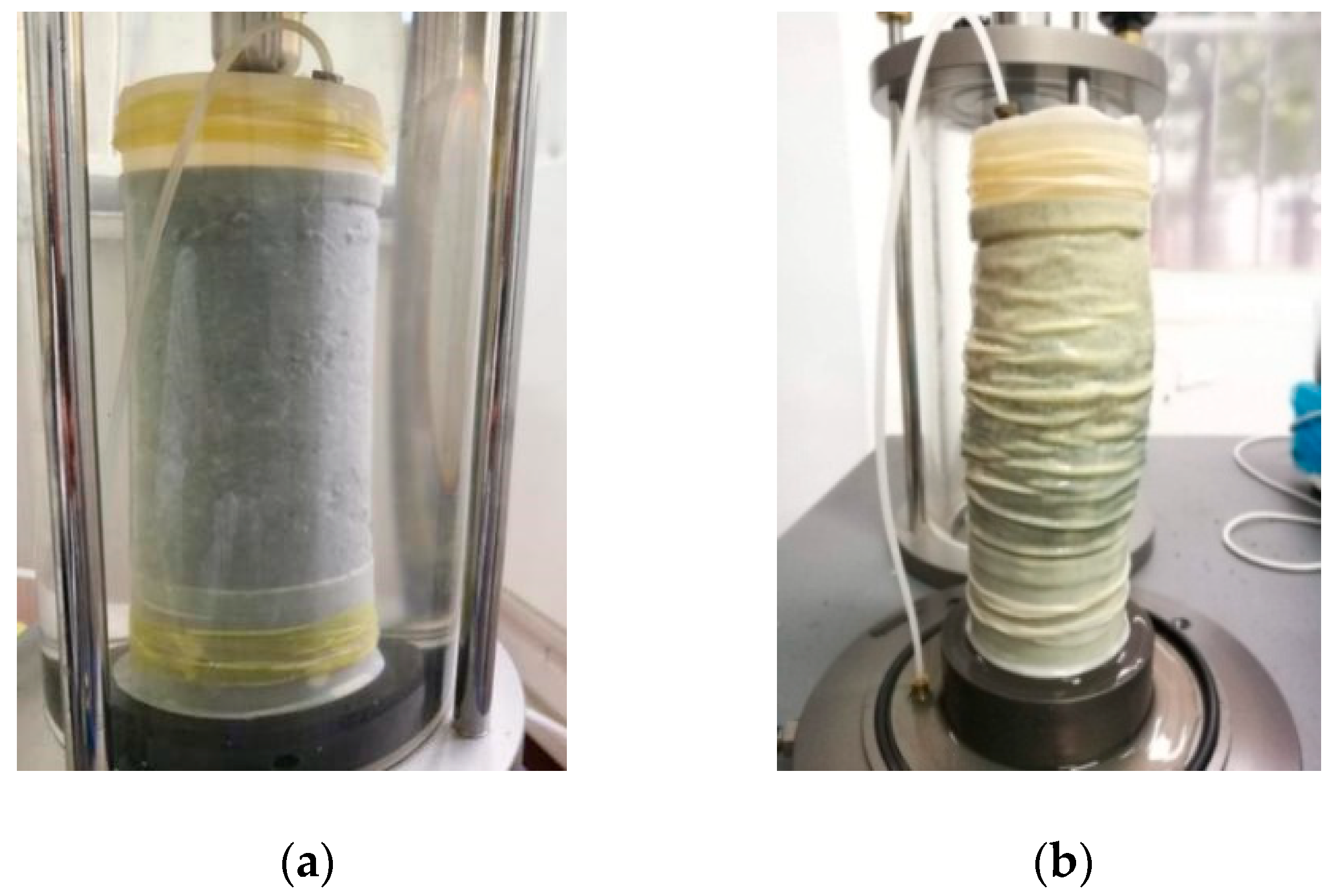
3.2. Strength Measurement of Soil–Rock Mixtures
3.2.1. Testing Process
3.2.2. Testing Scheme
3.3. Testing Results
4. Comparison with Liu’s Method
5. Slope Stability Analysis, Considering Rock Content
6. Discussion About Stability Estimation of the Soil–Rock Slope
6.1. Discussion About Characteristic Parameters of the Soil–Rock Slope
6.2. Discussion on the Applicability of Analytical Methods
- (1)
- In the process of sampling for stability analysis of soil–rock slopes, it is advised to survey in the main affecting area first, and then survey in the secondary affecting area. The definition of affecting area is shown in Figure 19, that L is the basic length [3,16]. In this process, L is the horizontal length of plastic belt to slope top in homogeneous soil slope models, and L is 4 m in the article.
- (2)
- When the rock size is 0.1~0.4 Ls (Ls is the width of slope) in the main affecting area, it is advised to use analysis models with the Monte Carlo method, considering the strengthening effect of rocks. When the soil–rock slope is more easily affected by rainfall, traffic load, and other factors, it is advised to use analysis models with the Monte Carlo method, considering the scatter strength of soil–rock mixtures. When the soil–rock interface is weak, it is advised to use analysis models with the Monte Carlo method, considering the weakening effects of soil–rock interface area.
7. Conclusions
- (1)
- The Monte Carlo method and its application in stability analysis of soil–rock slopes are introduced in detail.
- (2)
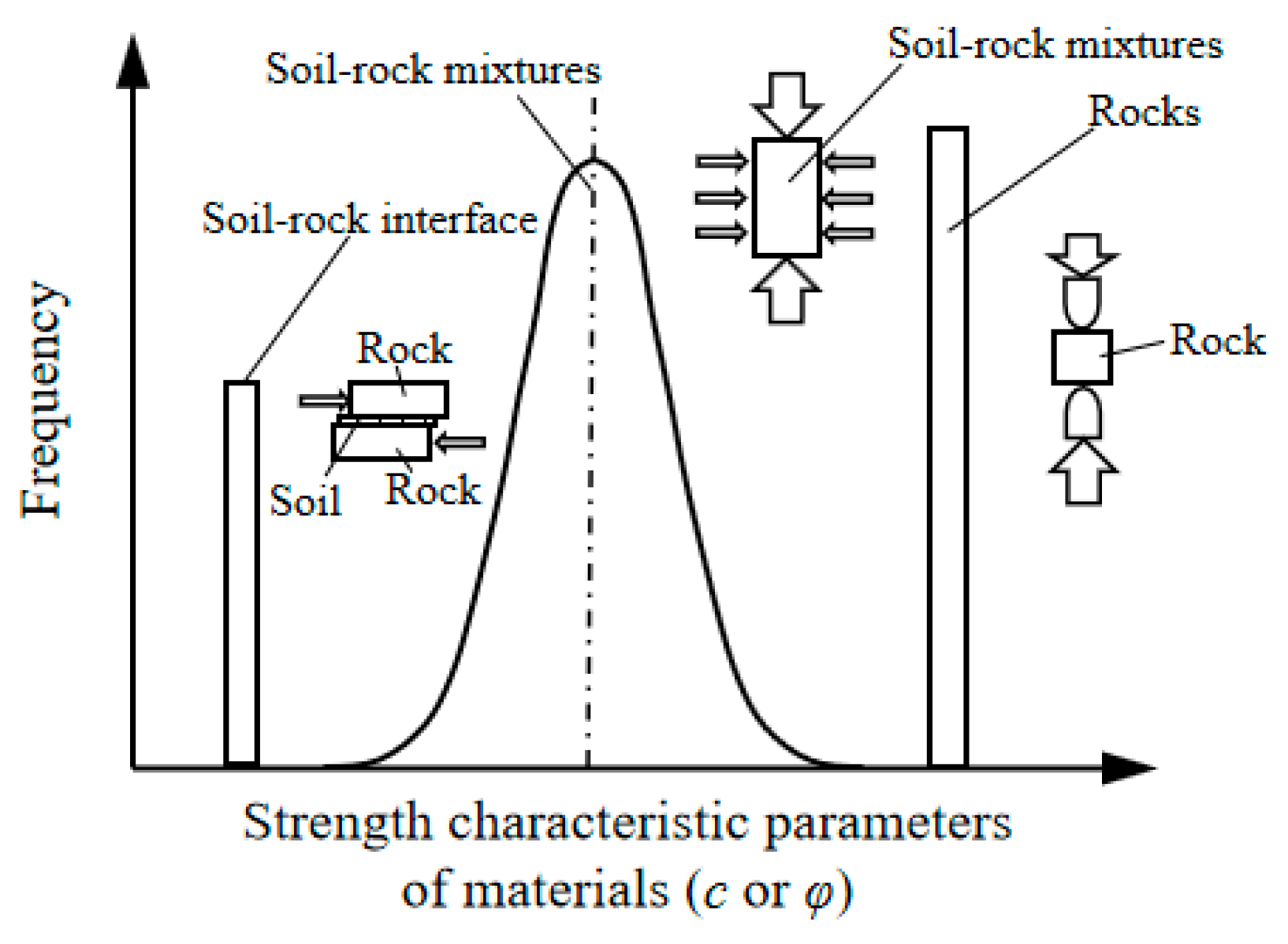
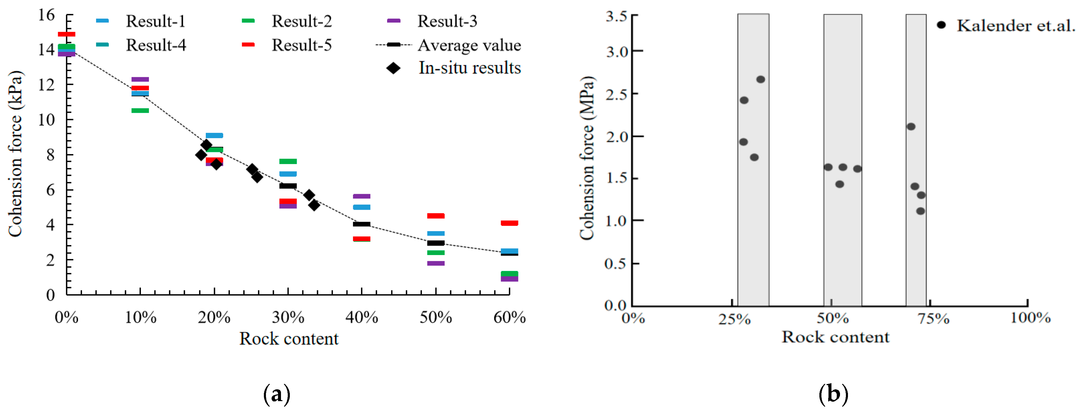
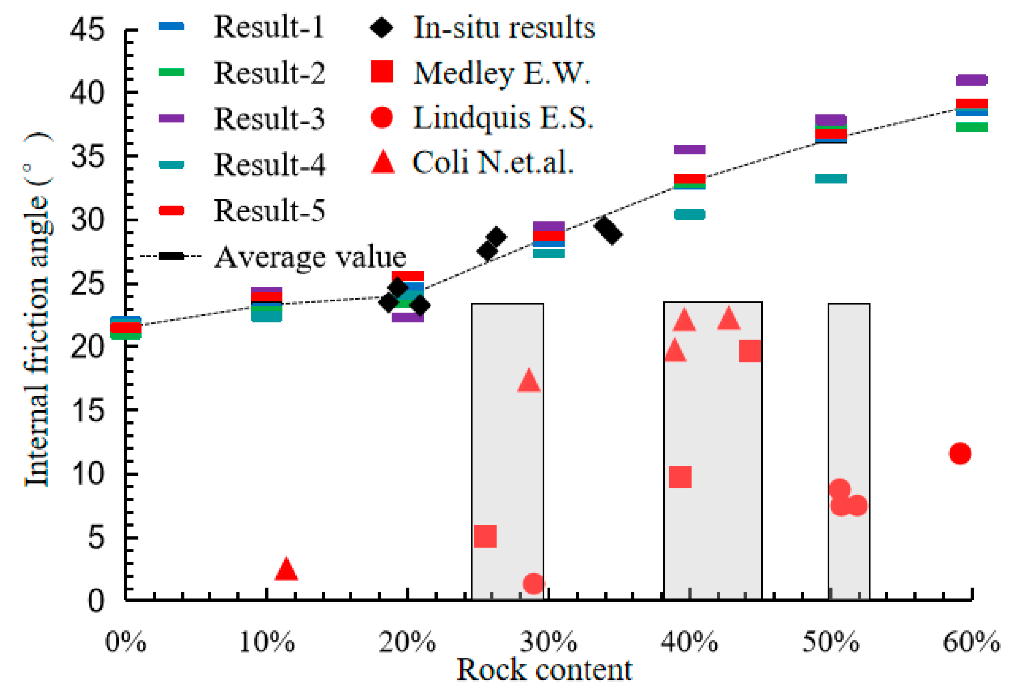
- Based on the strength of soil–rock mixtures arising from the in situ samples and remade samples, the scatter characteristic of cohesion and internal friction angle for soil–rock mixtures were proved, and it can be concluded that the cohesion reduces with the increase of rock content, and the internal friction angle increases with the increase of rock content.
- (3)
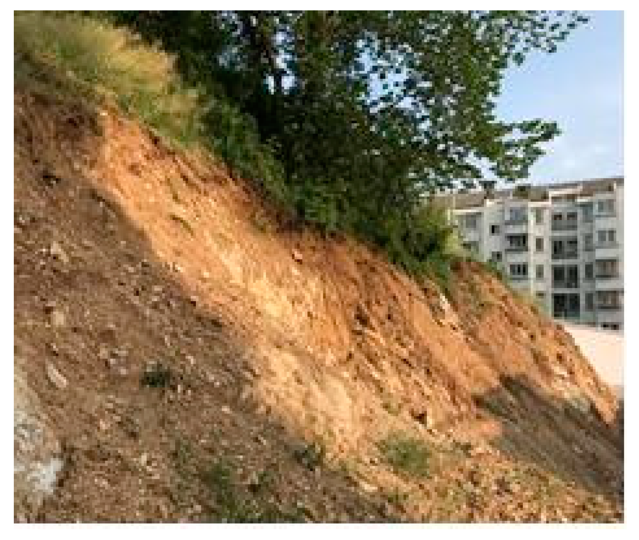
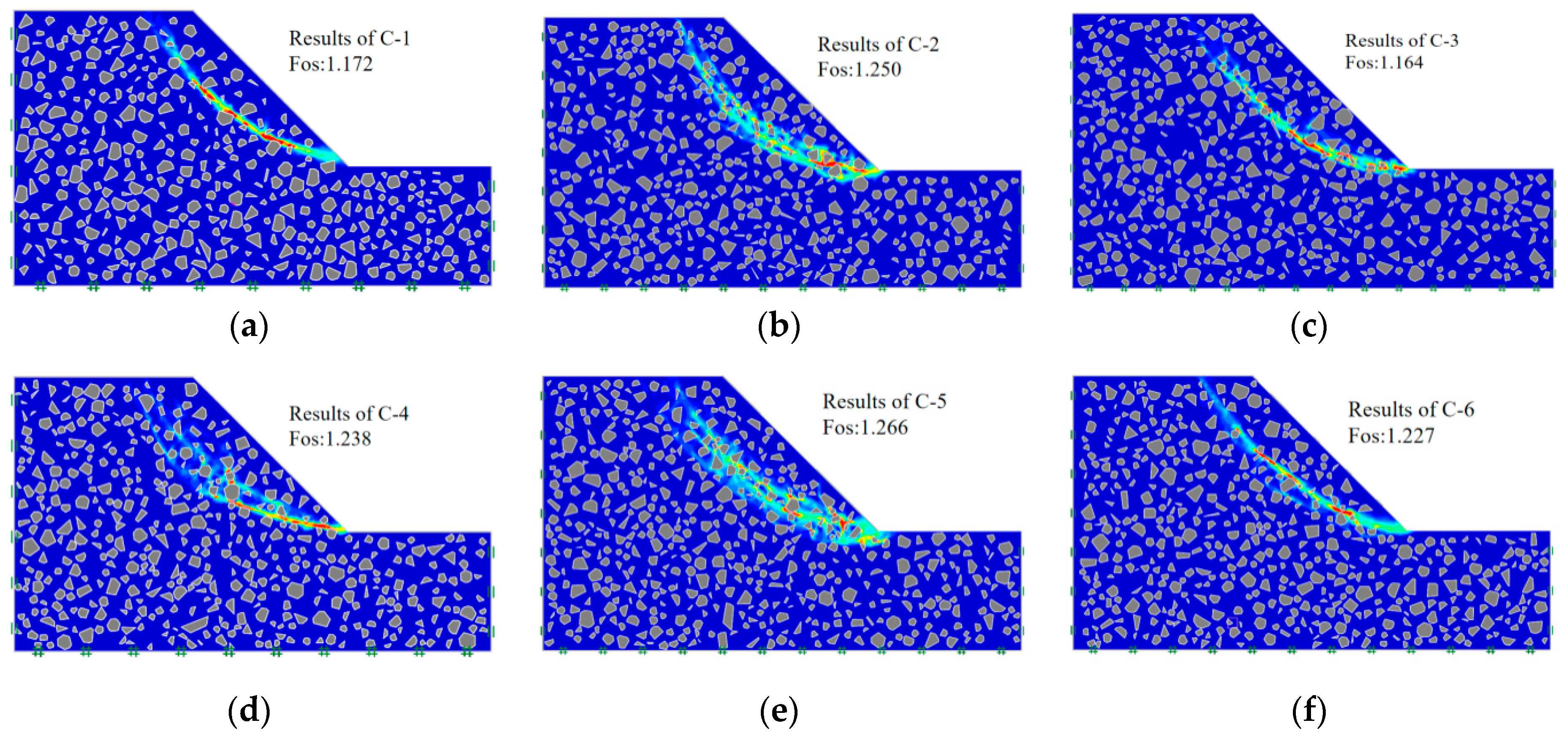
- Through comparing with the failed slope and Liu’s method for analyzing the stability of soil–rock slopes, it was proved that analyzing the soil–rock slope with the Monte Carlo method is reasonable and economical.
- (4)
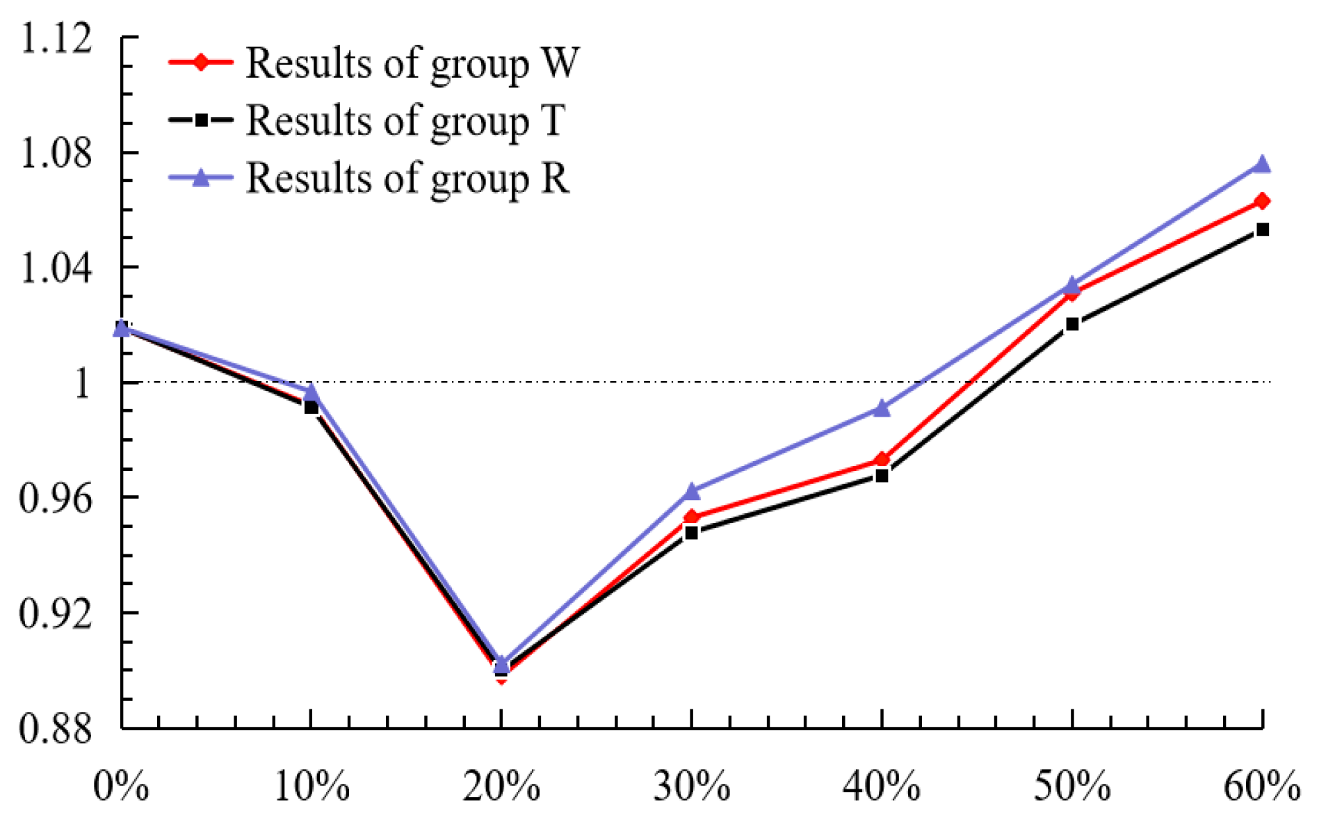
- The stability of the soil–rock slope, considering strengthening effect of rocks to slope and different rock contents, was studied, and the results show that with the increase of rock content, the stability of the soil–rock slope reduces first and then increases, and the minimum value was achieved at 20% rock content. When the rock content is over 30%, the soil–rock slope achieves the largest safety factor, when considering the strengthening effect of rocks, and achieves the smallest safety factor when considering the scatter strength of soil–rock mixtures.
- (5)
- Based on a large number of examples and existing documents, the investigation area for the optimum parameter characteristics of soil–rock mixture in slope stability analysis is proposed. Taking these into account, the chosen models were put forward for different situations, to study which situations are suitable for analysis models, considering the weak soil–rock interface area and the strengthening effect of rocks.
Author Contributions
Funding
Conflicts of Interest
References
- Xu, W.J.; Xu, Q.; Hu, R.L. Study on the shear strength of soil–rock mixture by large scale direct shear test. Int. J. Rock Mech. Min. Sci. 2011, 48, 1235–1247. [Google Scholar]
- Coli, N.; Berry, P.; Boldini, D. In situ non-conventional shear tests for the mechanical characterisation of a bimrock. Int. J. Rock Mech. Min. Sci. 2011, 48, 95–102. [Google Scholar] [CrossRef]
- Liu, S.Q.; Huang, X.W.; Zhou, A.Z.; Hu, J.; Wang, W. Soil-Rock Slope Stability Analysis by Considering the Nonuniformity of Rock. Math. Probl. Eng. 2018, 2018, 1–15. [Google Scholar] [CrossRef]
- Wang, Y.; Li, C.H.; Hu, Y.Z. Use of X-ray computed tomography to investigate the effect of rock blocks on meso-structural changes in soil-rock mixture under triaxial deformation. Constr. Build. Mater. 2018, 164, 386–399. [Google Scholar] [CrossRef]
- Zhang, H.; Xu, W.; Yu, Y. Triaxial tests of soil–rock mixtures with different rock block distributions. Soils Found. 2016, 56, 44–56. [Google Scholar] [CrossRef]
- Zhang, Y. Study on strength, deformation characteristics and interaction between soil and stone of soil-rock mixture. CET J. 2017, 59, 985–990. [Google Scholar]
- Wang, W.; Zhang, C.; Li, N.; Tao, F.F.; Yao, K. Characterisation of nano magnesia-cement-reinforced seashore soft soil by direct-shear test. Mar. Georesour. Geotec. 2019, 37, 989–998. [Google Scholar] [CrossRef]
- Kalender, A.; Sonmez, H.; Medley, E.; Tunusluoglu, C.; Kasapoglu, K.E. An approach to predicting the overall strengths of unwelded bimrocks and bimsoils. Eng. Geol. 2014, 183, 65–79. [Google Scholar] [CrossRef]
- Huang, D.; Gu, D.M. Influence of filling-drawdown cycles of the Three Gorges reservoir on deformation and failure behaviors of anaclinal rock slopes in the Wu Gorge. Geomorphology 2017, 295, 489–506. [Google Scholar] [CrossRef]
- Li, R.W.; Wang, N.Q. Landside susceptibility mapping for the muchuan county (China): A comparison between bivariate statistical models (WOE, EBF, and IOE) and their ensembles with logistic regression. Symmetry 2019, 11, 762. [Google Scholar] [CrossRef]
- Xu, W.J.; Hu, L.M.; Gao, W. Random generation of the meso-structure of a soil-rock mixture and its application in the study of the mechanical behavior in a landslide dam. Int. J. Rock Mechmin. 2016, 86, 166–178. [Google Scholar] [CrossRef]
- Gao, W.; Gao, W.; Hu, R.L.; Xu, P.; Xia, J. Microtremor survey and stability analysis of a soil-rock mixture landslide: A case study in Baidian town, China. Landslides 2018, 15, 1951–1961. [Google Scholar] [CrossRef]
- Yang, Y.; Sun, G.; Zheng, H.; Qi, Y. Investigation of the sequential excavation of a soil-rock-mixture slope using the numerical manifold method. Eng. Geol. 2019, 256, 93–109. [Google Scholar] [CrossRef]
- Khorasani, E.; Amini, M.; Hossaini, M.F.; Medley, E. Statistical analysis of bimslope stability using physical and numerical models. Eng. Geol. 2019. [Google Scholar] [CrossRef]
- Wang, T.; Zhang, G. Failure behavior of soil-rock mixture slopes based on centrifuge model test. J. Mt. Sci. Engl. 2019, 16, 1928–1942. [Google Scholar] [CrossRef]
- Napoli, M.L.; Barbero, M.; Ravera, E.; Scavia, C. A stochastic approach to slope stability analysis in bimrocks. Int. J. Rock Mech. Min. Sci. 2018, 10, 41–49. [Google Scholar] [CrossRef]
- Liu, Y.; Xiao, H.; Yao, K.; Hu, J.; Wei, H. Rock-soil slope stability analysis by two-phase random media and finite elements. Geosci. Front. 2018, 9, 1649–1655. [Google Scholar] [CrossRef]
- Meng, Q.X.; Wang, H.L.; Xu, W.Y.; Xu, J.; Cai, M.; Zhang, Q. Multiscale strength reduction method for heterogeneous slope using hierarchical FEM/DEM modeling. Comput. Geotech. 2019, 115, 103164. [Google Scholar] [CrossRef]
- Xu, H.F.; Liu, L.L.; Liu, Y. Water-induced changes in mechanical parameters of soil-rock mixture and their effect on talus slope stability. Geomech. Eng. 2019, 4, 353–362. [Google Scholar]
- Afifipour, M.; Moarefvand, P. Mechanical behavior of bimrocks having high rock block proportion. Int. J. Rock Mech. Min. Sci. 2014, 65, 40–48. [Google Scholar] [CrossRef]
- Huang, X.W.; Liu, S.Q.; Sui, X.L.; Hu, Y. Earthquake response analysis of soil-rock slope based on distribution of rocks. In Proceedings of the 2018 International Forum on Construction, Aviation and Environmental Engineering-Internet of Things, Guangzhou, China, 2 July 2018; p. 175. [Google Scholar]
- Hanif, M.H.; Adnan, M.; Shah, S.A.R.; Khan, N.M.; Nadeem, M.; Javed, J.; Akbar, M.W.; Farooq, A.; Waseem, M. Rainfall runoff analysis and systainable soil bed optumization engineering process: Application of an advanced decision-making technique. Symmetry 2019, 11, 1224. [Google Scholar] [CrossRef]
- Xiong, X.; Shi, Z.; Xiong, Y.; Peng, M.; Ma, X.; Zhang, F. Unsaturated slope stability around the Three Gorges Reservoir under various combinations of rainfall and water level fluctuation. Eng. Geol. 2019, 1, 105231. [Google Scholar] [CrossRef]
- Hoggan, P.E.; Brändas, E.J.; Maruani, J.; Piecuch, P.; Delgado-Barrio, G. Preface: Advances in the Theory of Quantum Systems in Chemistry and Physics; Springer: Berlin/Heidelberg, Germany, 2012. [Google Scholar]
- Cheng, Y.W.; Zhu, H.P.; Hu, K.; Wu, J.; Shao, X.Y. Reliability prediction of machinery with multiple degradation characteristics using double-Wiener process and Monte Carlo algorithm. Mech. Syst. Signal Pr. 2019, 134, 106333. [Google Scholar] [CrossRef]
- Liu, X.; Li, D.Q.; Cao, Z.J.; Wang, Y. Adaptive Monte Carlo simulation method for system reliability analysis of slope stability based on limit equilibrium methods. Eng. Geol. 2020, 264, 105384. [Google Scholar] [CrossRef]
- Pasculli, A.; Calista, M.; Sciarra, N. Variability of local stress states resulting from the application of Monte Carlo and finite difference methods to the stability study of a selected slope. Eng. Geol. 2018, 245, 370–389. [Google Scholar] [CrossRef]
- Dyson, A.P.; Tolooiyan, A. Prediction and classification for finite element slope stability analysis by random field comparison. Comput. Geotech. 2019, 109, 117–129. [Google Scholar] [CrossRef]
- Yao, K.; Chen, Q.; Xiao, H.; Liu, Y.; Lee, F.H. Small-strain shear modulus of cement-treated marine clay. J. Mater. Civil. Eng. 2020, 32, 04020114. [Google Scholar] [CrossRef]
- Yao, K.; An, D.L.; Wang, W.; Li, N.; Zhang, Z.; Zhou, A.Z. Effect of nano-mgo on mechanical performance of cement stabilized silty clay. Mar. Georesour. Geotec. 2020, 38, 250–255. [Google Scholar] [CrossRef]
- Wang, W.; Li, Y.; Yao, K.; Li, N.; Zhou, A.Z.; Zhang, Z. Strength properties of nano-MgO and cement stabilized coastal silty clay subjected to sulfuric acid attack. Mar. Georesour. Geotec. 2019. [Google Scholar] [CrossRef]
- Wang, W.; Fu, Y.; Zhang, Z.; Li, N.; Zhou, A.Z. Mathematical models for stress-strain behavior of nano magnesia-cement-reinforced seashore soft soil. Mathematics 2020, 8, 456. [Google Scholar] [CrossRef]
- Raphael, B.; Smith, I.F.C. A direct stochastic algorithm for global search. Appl. Math. Comput. 2003, 146, 729–758. [Google Scholar] [CrossRef]
- Thistleton, W.J.; Marsh, J.A.; Nelson, K. Generalized Box–Muller Method for Generating q-Gaussian Random Deviates. IEEE Trans. Inform. Theory 2007, 53, 4805–4810. [Google Scholar] [CrossRef]
- Rodrigues, D.J. A simple generalization of the Box–Muller method for obtaining a pair of correlated standard normal variables. J. Stat. Comput. Sim. 2010, 80, 953–958. [Google Scholar]
- Jakob, S.; Fabian, R.; Martin, S.; Jens, L. Significance of preferential flow at the rock soil interface in a semi-arid karst environment. Catena 2014, 123, 1–10. [Google Scholar]
- Ákos, T.; Gong, Q.M.; Zhao, J. Case studies of TBM tunneling performance in rock–soil interface mixed ground. Tunn. Undergr. Space Technol. 2013, 38, 140–150. [Google Scholar]
- Chang, W.; Phantachang, T. Effects of gravel content on shear resistance of gravelly soils. Eng. Geol. 2016, 207, 78–90. [Google Scholar] [CrossRef]
- Chinese National Geotechnical Test Standard, GB/T 50123-1999. China Planning Press, 1999. Available online: http://www.zys168.net/Upload/DownLoad/DownLoadFile/20107191920846.pdf (accessed on 26 October 2019). (In Chinese).
- Meng, Q.X.; Wang, H.L.; Xu, W.Y.; Cai, M. A numerical homogenization study of the elastic property of a soil-rock mixture using random mesostructure generation. Comput. Geotech. 2018, 98, 48–57. [Google Scholar] [CrossRef]
- Zhang, W.J.; Qing, L.; Li, H.L. Research on shear behavior characteristics of soil-rock mixture. Int. J. Earth Sci. 2015, 6, 2620–2625. [Google Scholar]
- Gong, J.; Liu, J. Analysis on the Mechanical Behaviors of Soil-rock Mixtures Using Scatter Element Method. Procedia Eng. 2015, 102, 1783–1792. [Google Scholar] [CrossRef]
- Huang, X.W.; Zhou, A.Z.; Wang, W.; Jiang, P.M. Characterization of the dynamic properties of clay–gravel mixtures at low strain level. Sustainability 2020, 12, 1616. [Google Scholar] [CrossRef]
- Qian, Z.G.; Li, A.J.; Chen, W.C.; Lyamin, A.V.; Jiang, J.C. An artificial neural network approach to inhomogeneous soil slope stability predictions based on limit analysis methods. Soils Found. 2019, 59, 556–569. [Google Scholar] [CrossRef]


| Specimen | Physical Parameters | ||||
|---|---|---|---|---|---|
| clay | Specific Gravity | Liquid Limit | Plastic Limit | Plasticity Index | Optimized Water Content |
| 2.75 | 41.30% | 19.20% | 22.10% | 16% | |
| rock | Point pressure strength | crushing index | Density | ||
| 1234 N | 23% | 2.6 g/cm3 | |||
| In Situ Samples | Remade Samples | ||
|---|---|---|---|
| Number | Rock Content | Number | Rock Content |
| I-1 | 18.4 | R-0-1/2/3/4/5 | 0% |
| I-2 | 18.7 | R-1-1/2/3/4/5 | 10% |
| I-3 | 20.3 | R-2-1/2/3/4/5 | 20% |
| I-4 | 25.2 | R-3-1/2/3/4/5 | 30% |
| I-5 | 25.9 | R-4-1/2/3/4/5 | 40% |
| I-6 | 32.9 | R-5-1/2/3/4/5 | 50% |
| I-7 | 33.7 | R-6-1/2/3/4/5 | 60% |
| Number | VBP | Time (s) | Safety Factor | Number | VBP | Time (s) | Safety Factor |
|---|---|---|---|---|---|---|---|
| C-1 | 22.50% | 163 | 1.172 | C-4 | 22.40% | 140 | 1.238 |
| C-2 | 22.00% | 135 | 1.25 | C-5 | 23.10% | 149 | 1.266 |
| C-3 | 22.50% | 128 | 1.164 | C-6 | 22.80% | 146 | 1.227 |
| Number | Cohesion (kPa) | Internal Friction Angle (°) | Standard Deviation of Cohesion (kPa) | Standard Deviation of Internal Friction Angle (°) | Time (s) | Repeated Times | Safety Factor | Standard Deviation of Safety Factor |
|---|---|---|---|---|---|---|---|---|
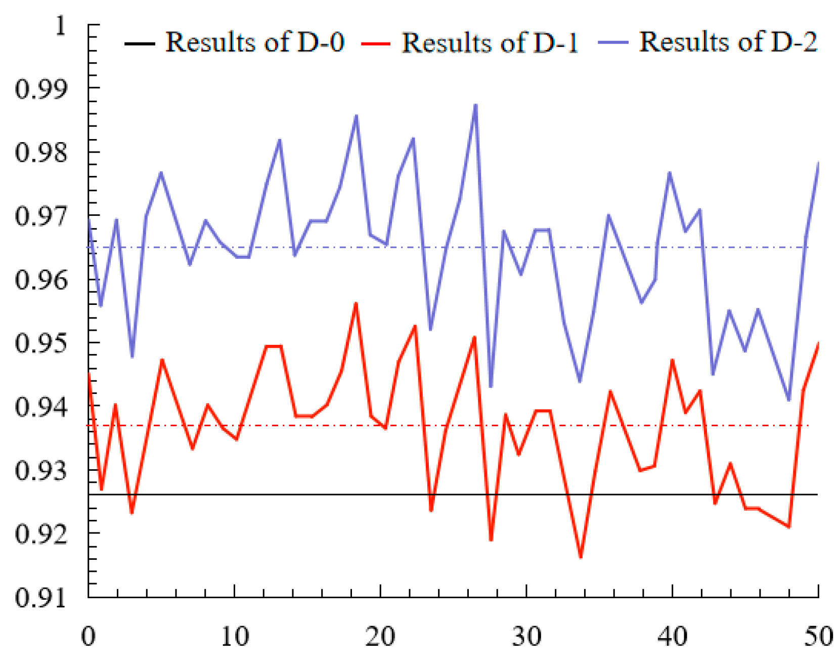
| D-0 | 7.3 | 26.4 | 0 | 0 | 47s | 1 | 0.929 | 0 |
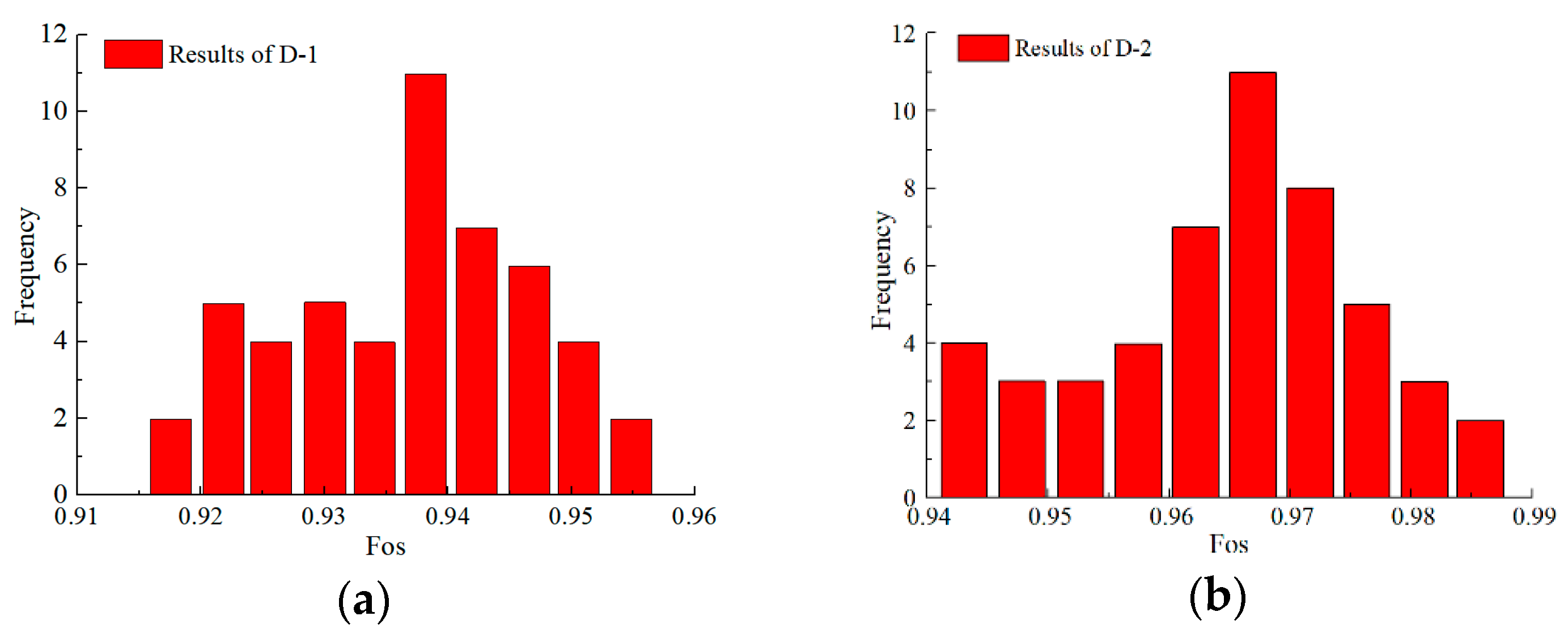
| D-1 | 7.3 | 26.4 | 0.9 | 1.05 | 953 | 50 | 0.937 | 0.00959 |
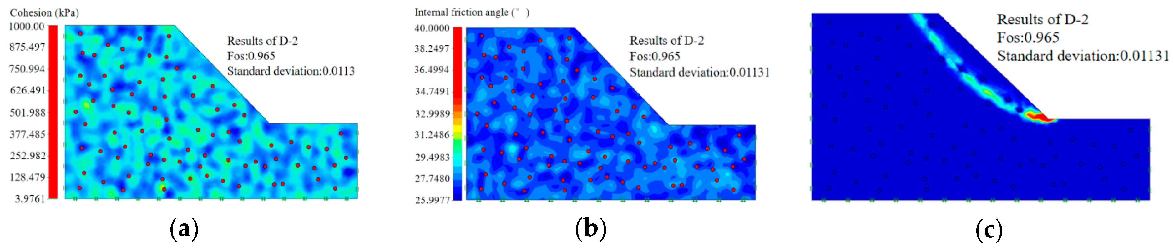
| D-2 | 7.3 | 26.4 | 0.9 | 1.05 | 965 | 50 | 0.965 | 0.01131 |
| Number | MBP | Cohesion (kPa) | Internal Friction Angle (°) | Safety Factor |
|---|---|---|---|---|
| W-0 | 0% | 14.1 | 21.5 | 1.019 |
| W-1 | 10% | 11.5 | 23.3 | 0.992 |
| W-2 | 20% | 8.6 | 24 | 0.898 |
| W-3 | 30% | 6.2 | 28.7 | 0.953 |
| W-4 | 40% | 4.0 | 33 | 0.973 |
| W-5 | 50% | 3.1 | 36.4 | 1.031 |
| W-6 | 60% | 2.4 | 39 | 1.063 |
| Number | MBP | Cohesion (kPa) | Internal Friction Angle (°) | Standard Deviation of Cohesion (kPa) | Standard Deviation of Internal Friction Angle (°) | Average Safety Factor | Standard Deviation |
|---|---|---|---|---|---|---|---|
| T-0 | 0% | 14.1 | 21.5 | 0.3 | 0.3 | 1.019 | 0.00312 |
| T-1 | 10% | 11.5 | 23.3 | 0.6 | 0.6 | 0.9914 | 0.00461 |
| T-2 | 20% | 8.6 | 24 | 0.8 | 0.9 | 0.8999 | 0.00597 |
| T-3 | 30% | 6.2 | 28.7 | 1.0 | 1.2 | 0.9479 | 0.01262 |
| T-4 | 40% | 4.0 | 33 | 1.2 | 1.5 | 0.9678 | 0.02470 |
| T-5 | 50% | 3.1 | 36.4 | 1.4 | 1.8 | 1.02 | 0.03866 |
| T-6 | 60% | 2.4 | 39 | 1.6 | 2.1 | 1.053 | 0.04056 |
| Number | MBP | Cohesion (kPa) | Internal Friction Angle (°) | Standard Deviation of Cohesion (kPa) | Standard Deviation of Internal Friction Angle (°) | Probability of Rock | Average Safety Factor | Standard Deviation |
|---|---|---|---|---|---|---|---|---|
| R-0 | 0% | 14.1 | 21.5 | 0.3 | 0.3 | 0% | 1.019 | 0.00312 |
| R-1 | 10% | 11.5 | 23.3 | 0.6 | 0.6 | 10% | 0.9968 | 0.00391 |
| R-2 | 20% | 8.6 | 24 | 0.8 | 0.9 | 20% | 0.9022 | 0.00666 |
| R-3 | 30% | 6.2 | 28.7 | 1.0 | 1.2 | 30% | 0.9623 | 0.00934 |
| R-4 | 40% | 4.0 | 33 | 1.2 | 1.5 | 40% | 0.9912 | 0.02525 |
| R-5 | 50% | 3.1 | 36.4 | 1.4 | 1.8 | 50% | 1.034 | 0.04049 |
| R-6 | 60% | 2.4 | 39 | 1.6 | 2.1 | 60% | 1.076 | 0.04573 |
© 2020 by the authors. Licensee MDPI, Basel, Switzerland. This article is an open access article distributed under the terms and conditions of the Creative Commons Attribution (CC BY) license (http://creativecommons.org/licenses/by/4.0/).
Share and Cite
Zhou, A.; Huang, X.; Li, N.; Jiang, P.; Wang, W. A Monte Carlo Approach to Estimate the Stability of Soil–Rock Slopes Considering the Non-Uniformity of Materials. Symmetry 2020, 12, 590. https://doi.org/10.3390/sym12040590
Zhou A, Huang X, Li N, Jiang P, Wang W. A Monte Carlo Approach to Estimate the Stability of Soil–Rock Slopes Considering the Non-Uniformity of Materials. Symmetry. 2020; 12(4):590. https://doi.org/10.3390/sym12040590
Chicago/Turabian StyleZhou, Aizhao, Xianwen Huang, Na Li, Pengming Jiang, and Wei Wang. 2020. "A Monte Carlo Approach to Estimate the Stability of Soil–Rock Slopes Considering the Non-Uniformity of Materials" Symmetry 12, no. 4: 590. https://doi.org/10.3390/sym12040590
APA StyleZhou, A., Huang, X., Li, N., Jiang, P., & Wang, W. (2020). A Monte Carlo Approach to Estimate the Stability of Soil–Rock Slopes Considering the Non-Uniformity of Materials. Symmetry, 12(4), 590. https://doi.org/10.3390/sym12040590