Optimization Analysis of the N Policy M/G/1 Queue with Working Breakdowns

Abstract

This paper deals with the N policy M/G/1 queue with working breakdowns. The supplementary variable and probability generating function techniques are implemented to develop the steady-state results. The stability condition of a stable queue, as well as several system performance measures, are also derived. A two-stage optimization method is employed to determine the optimal threshold N and the optimal joint values of two mean service rates until the stability constraint is satisfied. To demonstrate the effectiveness of two-stage optimization method, some numerical results are presented. Finally, we carry out sensitivity analysis for the expected cost function with numerical illustrations.

1. Introduction

This paper investigates optimization analysis of the N-policy M/G/1 queue with working breakdowns. The N-policy introduced by Yadin and Naor [1] is used to turn a server on when the total number of customers in the system reaches a threshold $N$ ($N\ge 1$), and to turn a server off when there are no customers in the system. There is extensive literature on the N-policy queue, which has been studied by many researchers (see a recent survey by Jayachitra and Albert [2] and the references cited therein). In many practical situations, servers break down at any time while in operation; however, they still work at a lower service rate rather than completely stopping service during the breakdown period. This is called a working breakdown, as first introduced by Kalidass and Kasturi [3]. Based on the matrix analytic method, Liou [4] found the steady-state probabilities of the number of customers in the M/M/1 queue with working breakdowns and impatient customers. Kim and Lee [5] analyzed the M/G/1 queue with disasters and working breakdowns, and derived the system size distribution and the sojourn time distribution, respectively.

The N-policy, T-policy, and the Min (N, T)-policy M/G/1 queues with unreliable servers were proposed by Wang and Ke [6]. For the T-policy, the server takes a “vacation” of a fixed length T if there are no customers in the system. When the vacation ends, the server returns from vacation and works as long as there is at least one customer in the system. Otherwise, it takes another vacation of fixed length T until at least one customer is present in the system. Moreover, the Min (N, T) policy means that the server starts working if either the condition of the N-policy or the T-policy is satisfied. For these three queues, they showed the steady-state probability that the server is busy, which is equal to the traffic intensity. Wang [7] developed the exact steady-state solutions of the N-policy M/M/1 queue with server breakdowns. The N-policy M/M/1 queue with heterogeneous arrival rates, server breakdowns, and vacations was analyzed by Ke and Pearn [8]. Wang et al. [9] utilized the principle of maximum entropy to investigate the N-policy M/G/1 queue with server breakdowns and general startup times. Using the same approach, Ke and Lin [10] approximated the steady-state probability distributions of the queue length for the N-policy M^[x]/G/1 queue with an unreliable server and a single vacation. The optimal control of the N-policy M/G/1 queueing system with server breakdowns and general startup times was examined by Wang et al. [11]. They applied the direct search method to determine the optimal threshold N at the minimum cost. Jain and Bhargava [12] performed cost analysis of the N-policy for the machine repair problem with mixed standbys and an unreliable server. An N-policy M^X/M/1 queueing system with server startup and breakdowns was analyzed by Vemuri et al. [13], where service was in two phases. Singh et al. [14] focused on the investigation of the N-policy queue with an unreliable server, state-dependent arrival rates, two phases of service, and m phases of repair. Moreover, Yang and Ke [15] applied the supplementary variable technique to analyze the (p, N)-policy M/G/1 queue with an unreliable server and a single vacation. Chen and Wang [16] address the sensitivity analyses of a retrial machine repair problem with warm standby units and a single server under the N-policy.

Over the years, there has been extensive literature on N-policy queues with server breakdowns, in which the server stops working completely during the breakdown period. However, there are no studies investigating the N-policy queue with working breakdowns. This queueing model accommodates many real-world systems, such as computer systems, assembly systems, and manufacturing systems. Thus, it motivates us to focus on the analysis of the N-policy M/G/1 queue with working breakdowns. The purpose of this paper is three-fold.

(1)

We derive several system performance measures, as well as the stability condition of this queueing model;

(2)

We establish a cost model to find the optimal threshold N, the optimal service rate during the normal period, and the optimal service rate during the working breakdown period under the stability condition;

(3)

We apply the two-stage optimization method to search for the minimum expected cost. Numerical examples are given to illustrate the effectiveness of the two-stage optimization method. Moreover, a sensitivity analysis is also performed.

2. Model Descriptions

We consider the N-policy M/G/1 queue with working breakdowns. It is assumed that customers arrive following a Poisson process with parameter $\lambda$. We assume that the service times in the normal and working breakdown states are independent and identically distributed (i.i.d.) random variables that obey arbitrary distribution functions $B_1(x)$ and $B_2(x),$ respectively, with respective mean service rates ${\mu }_1$ and ${\mu }_2$. The Laplace–Stieltjes transforms of $B_1(x)$ and $B_2(x)$ are denoted by $B_1^{\ast }(\theta )$ and $B_2^{\ast }(\theta )$, respectively. The server can serve only one customer at a time. Meanwhile, arriving customers form a single waiting line based on the first-come, first-served (FCFS) discipline. The server may suffer from failure at any time with Poisson breakdown rate $\alpha$ when it is turned on and working. Whenever the server fails, it is immediately repaired at a repair rate $\beta$, and repair times are assumed to be exponentially distributed. Arriving customers that find the server busy immediately join the queue until the server is available. During the server breakdown period, customers continue to enter the system according to a Poisson process. Once the server recovers to a normal state, it immediately serves a customer with a fast service rate ${\mu }_1$. Otherwise, the failed server would be repaired and then turned off when no customers are in the system. Moreover, we assume that various stochastic processes involved in this queueing system are independent of each other.

Practical Justification of the Model

Cloud computing is the latest major computing paradigm, which shifts the deployment of computing infrastructure (such as CPU, network, and storage) from end users to the cloud data center. Computing infrastructure is virtualized in cloud computing, and therefore all cloud services are provided by virtual machines (VM), virtual networks, and virtual storage. Cloud service providers offer a VM for each cloud service request, and each VM consists of a kernel program and a root file system, with at least 5 GB disk space. As more cloud users arrive, the simultaneous disk access becomes the performance bottleneck in cloud computing. To guarantee the availability and reliability of cloud services, cloud providers usually establish distributed storage to improve storage efficiency. A practical situation related to the distributed storage system is presented for illustrative purposes. Consider a data center built and managed by the CloudStack cloud computing management system providing a platform as a service (PaaS). To increase the disk access bandwidth, a Ceph distributed storage cluster is integrated into the CloudStack cloud environment. Figure 1 depicts the system architecture of this data center. The Ceph storage cluster consists of one Ceph monitor (MON), which maintains a copy of the cluster map, and four Ceph object store daemons (OSD), which store data as objects on a storage node.

To decrease the power consumption, the Ceph storage cluster is off at the outset. Assume that the arrival of PaaS request follows the exponential distribution with parameter $\lambda$. Upon the arrival of a request, the CloudStack will deploy a VM with a root file system stored in the local disk. The Ceph storage cluster will be turned on when the number of PaaS requests exceeds the predefined threshold ($N$), and therefore CloudStack allocates root file systems in the Ceph storage cluster. Also, the Ceph storage cluster operates at an exponentially distributed full-speed disk access rate ${\mu }_1$ when four OSDs are working properly, while it operates at an exponentially distributed lower speed disk access rate ${\mu }_2$ if some of the OSDs fail, with exponentially distributed failure rate $\alpha$. The system manager requires an exponentially distributed repair time with mean $1/\beta$ to replace a failed OSD with a new one. The Ceph storage cluster will be shut off when none of VMs use its disk space.

3. Steady-State Results

Let $C(t)$ be the server status at time t. Then, we get (i) $C(t)=$ 0 if the server is turned off; (ii) $C(t)=$ 1 if the server is turned on and working; and (iii) $C(t)=$ 2 if the server is turned on but subject to working breakdowns.

Here, we let the supplementary variable $\zeta$ be the remaining service time for the customer in service. Then, the state of the system at time $t$ is given by $K(t)$ $\equiv$ number of customers in the system; $X(t)$ $\equiv$ remaining service time when the server is turned on and working; $Y(t)$ $\equiv$ remaining service time when the server is turned on but subject to working breakdowns; and $\zeta (t)$$\equiv$ remaining service time for the customer being served.

Let

$$\zeta (t)=\{\begin{array}{c}0,\\ X(t),\\ 0,\\ Y(t),\end{array}\begin{array}{c}\hspace{1em}\hspace{1em}\hspace{1em}C(t)=0,0\le K(t)\le N-1,\\ C(t)=1,K(t)\ge 1,\\ C(t)=2,K(t)=0,\\ C(t)=2,K(t)\ge 1.\end{array}$$

Then, $\left\{\left(C(t),K(t),\zeta (t)\right),t\ge 0\right\}$ is a continuous time Markov chain. Let us define

$$P_{0,n}(t)=\mathrm{Prob}\left\{C(t)=0,K(t)=n\right\},0\le n\le N-1$$

$$P_{1,n}(x,t)dx=\mathrm{Prob}\left\{C(t)=1,K(t)=n,x\le \zeta (t)\le x+dx\right\},n\ge 1,x>0,$$

$$P_{2,0}(t)=\mathrm{Prob}\left\{C(t)=2,K(t)=0\right\}$$

$$P_{2,n}(x,t)dx=\mathrm{Prob}\left\{C(t)=2,K(t)=n,x\le \zeta (t)\le x+dx\right\},n\ge 1,x>0,$$

In a steady state, we define the limiting probabilities $P_{0,n}=\underset{t\to \infty }{\lim }{P}_{0,n}(t)$ for $0\le n\le N-1$; $P_{2,0}=\underset{t\to \infty }{\lim }{P}_{2,0}(t)$; and $P_{i,n}(x)=\underset{t\to \infty }{\lim }{P}_{i,n}(x,t)$ for $i=1,2$, $x>0$, $n\ge 1$.

3.1. Steady-State Probability Equations

Using the arguments of Cox [17], the Kolmogorov forward equations for this queueing model under the stability condition are given by

$$\lambda P_{0,0}={\displaystyle {\int }_0^{\infty }{P}_{1,1}(x){\mu }_1(x)dx}+\beta P_{2,0},$$

(1)

$$\lambda P_{0,n}=\lambda P_{0,n-1},1\le n\le N-1,$$

(2)

$$(\lambda +\beta )P_{2,0}={\displaystyle {\int }_0^{\infty }{P}_{2,1}(x){\mu }_2(x)dx},$$

(3)

$$\frac{d}{dx}{P}_{1,n}(x)=-[\lambda +\alpha +{\mu }_1(x)]P_{1,n}(x)+(1-{\delta }_{1,n})\lambda P_{1,n-1}(x),n\ge 1,$$

(4)

$$\frac{d}{dx}{P}_{2,n}(x)=-[\lambda +\beta +{\mu }_2(x)]P_{2,n}(x)+(1-{\delta }_{1,n})\lambda P_{2,n-1}(x),n\ge 1,$$

(5)

The above equations are solved under the following boundary conditions at $x>0.$

$$P_{1,n}(0)={\displaystyle {\int }_0^{\infty }{P}_{1,n+1}(x){\mu }_1(x)dx}+\beta {\displaystyle {\int }_0^{\infty }{P}_{2,n}(x){\mu }_1(x)dx}+{\delta }_{N,n}\lambda P_{0,N-1},n\ge 1,$$

(6)

$$P_{2,n}(0)={\displaystyle {\int }_0^{\infty }{P}_{2,n+1}(x){\mu }_2(x)dx}+\alpha {\displaystyle {\int }_0^{\infty }{P}_{1,n}(x)dx}+{\delta }_{1,n}\lambda P_{2,0},n\ge 1,$$

(7)

where

$${\delta }_{n,i}=\{\begin{array}{c}1\hspace{1em}ifi=n\\ 0\hspace{1em}ifi\ne n\end{array}$$

3.2. Probability Generating Function

The probability generating function (p.g.f.) technique is used to derive analytic solutions $P_{0,0}$ and $P_{2,0}$ in neat closed-form expressions. The respective probability generating functions of $P_{0,n}$, $P_{1,n}$, and $P_{2,n}$ are defined as follows:

$$G_0(z)={\displaystyle \sum _{n=0}^{N-1}{z}^n{P}_{0,n}},\left|z\right|\le 1,$$

$$G_1(x,z)={\displaystyle \sum _{n=1}^{\infty }{z}^n{P}_{1,n}(x)},\left|z\right|\le 1,$$

$$G_2(x,z)={\displaystyle \sum _{n=1}^{\infty }{z}^n{P}_{2,n}(x)},\left|z\right|\le 1.$$

We express $G_0(z)$ in terms of $P_{0,0}$ as

$$G_0(z)=P_{0,0}{\displaystyle \sum _{n=0}^{N-1}{z}^n}=P_{0,0}\frac{1-z^N}{1-z}=P_{0,0}{\theta }_N(z),$$

(8)

where

$${\theta }_N(z)=\frac{1-z^N}{1-z}$$

Equation (4) is multiplied by $z^n$ $(n=1,2,\dots )$, and then the equations are added term by term. We finally get

$$\frac{\partial }{\partial x}{G}_1(x,z)=-[\lambda (1-z)+\alpha +{\mu }_1(x)]G_1(x,z).$$

(9)

Similarly, Equation (5) is multiplied by $z^n$ $(n=1,2,\dots )$, and then the equations are added term by term. We finally obtain

$$\frac{\partial }{\partial x}{G}_2(x,z)=-[\lambda (1-z)+\beta +{\mu }_2(x)]G_2(x,z).$$

(10)

Equations (6) and (7) are multiplied by $z^n$ $(n=1,2,\dots )$, and then the equations are added term by term. We finally get

$$\lambda P_{0,0}z+z{G}_1(0,z)=\beta P_{2,0}z+\lambda P_{0,0}{z}^{N+1}+{\displaystyle {\int }_0^{\infty }{G}_1(x,z){\mu }_1(x)dx}+\beta z{\displaystyle {\int }_0^{\infty }{G}_2(x,z)dx},$$

(11)

and

$$(\lambda +\beta )P_{2,0}z+z{G}_2(0,z)=\lambda P_{2,0}{z}^2+{\displaystyle {\int }_0^{\infty }{G}_2(x,z){\mu }_2(x)dx}+\alpha z{\displaystyle {\int }_0^{\infty }{G}_1(x,z)dx}.$$

(12)

Solving Equations (9) and (10) yields

$$G_1(x,z)=G_1(0,z)e^{-[\lambda (1-z)+\alpha ]x}[1-B_1(x)],$$

(13)

and

$$G_2(x,z)=G_2(0,z)e^{-[\lambda (1-z)+\beta ]x}[1-B_2(x)].$$

(14)

Substituting Equations (13) and (14) into Equations (11) and (12) yields

$$[z-B_1^{\ast }(\lambda (1-z)+\alpha )]G_1(0,z)-\beta z\frac{1-B_2^{\ast }(\lambda (1-z)+\beta )}{\lambda (1-z)+\beta }{G}_2(0,z)=\lambda z(z^N-1)P_{0,0}+\beta z{P}_{2,0},$$

(15)

And

$$-\alpha z\frac{1-B_1^{\ast }(\lambda (1-z)+\alpha )}{\lambda (1-z)+\alpha }{G}_1(0,z)+[z-B_2^{\ast }(\lambda (1-z)+\beta )]G_2(0,z)=\left[\lambda (z-1)-\beta \right]z{P}_{2,0}.$$

(16)

We define the following notations:

$$\begin{gathered} B_1^{\ast }\equiv B_1^{\ast }[\lambda (1-z)+\alpha ], \\ {B}_2^{\ast }\equiv B_2^{\ast }[\lambda (1-z)+\beta ], \\ {\theta }_{\alpha }(z)\equiv [\lambda (1-z)+\alpha ] \\ {\theta }_{\beta }(z)\equiv [\lambda (1-z)+\beta )] \end{gathered}$$

Using Cramer’s rule to solve Equations (15) and (16), we obtain the expressions for

$$G_1(0,z)=\frac{z(z-1){\theta }_{\alpha }(z){\theta }_{\beta }(z)\left[\lambda {\theta }_N(z)(z-B_2^{\ast })P_{0,0}+\beta B_2^{\ast }{P}_{2,0}\right]}{(z-B_1^{\ast })(z-B_2^{\ast }){\theta }_{\alpha }(z){\theta }_{\beta }(z)-\alpha \beta z^2(1-B_1^{\ast })(1-B_2^{\ast })},$$

(17)

and

$$G_2(0,z)=\frac{z{\theta }_{\beta }(z)\left\{\alpha \lambda z(1-B_1^{\ast })(z^N-1)P_{0,0}+\left[\alpha \beta z(1-B_1^{\ast })-(z-B_1^{\ast }){\theta }_{\alpha }(z){\theta }_{\beta }(z)\right]P_{2,0}\right\}}{(z-B_1^{\ast })(z-B_2^{\ast }){\theta }_{\alpha }(z){\theta }_{\beta }(z)-\alpha \beta z^2(1-B_1^{\ast })(1-B_2^{\ast })}.$$

(18)

Substituting Equations (17) and (18) into Equations (13) and (14), we obtain

$$G_1(z)=\frac{z(z-1){\theta }_{\beta }(z)(1-B_1^{\ast })\left[\lambda {\theta }_N(z)(z-B_2^{\ast })P_{0,0}+\beta B_2^{\ast }{P}_{2,0}\right]}{(z-B_1^{\ast })(z-B_2^{\ast }){\theta }_{\alpha }(z){\theta }_{\beta }(z)-\alpha \beta z^2(1-B_1^{\ast })(1-B_2^{\ast })},$$

(19)

and

$$G_2(z)=\frac{z(1-B_2^{\ast })\left\{\alpha \lambda z(1-B_1^{\ast })(z^N-1)P_{0,0}+\left[\alpha \beta z(1-B_1^{\ast })-(z-B_1^{\ast }){\theta }_{\alpha }(z){\theta }_{\beta }(z)\right]P_{2,0}\right\}}{(z-B_1^{\ast })(z-B_2^{\ast }){\theta }_{\alpha }(z){\theta }_{\beta }(z)-\alpha \beta z^2(1-B_1^{\ast })(1-B_2^{\ast })}.$$

(20)

The denominator of $G_1(z)$ has one of its roots (say) $z=r_1$ between 0 and 1. Since $G_1(z)\ge 0$, for $0\le z\le 1$, the numerator of $G_1(z)$ must vanish at $z=r_1$. Therefore

$$P_{2,0}=\frac{\lambda {\theta }_N(r_1)\left\{B_2^{\ast }[\lambda (1-r_1)+\beta ]-r_1\right\}}{\beta B_2^{\ast }[\lambda (1-r_1)+\beta ]}{P}_{0,0},$$

(21)

where

$${\theta }_N(r_1)=\frac{1-r_1{}^N}{1-r_1}.$$

It should be noted that when $N=1$ and $B_2^{\ast }\left(s\right)=\frac{{\mu }_2}{s+{\mu }_2}$, the expression in Equation (21) for $P_{2,0}$ is identical to the existing result in the literature (see Kalidass and Kasturi [3]).

Let $G(z)$ be the p.g.f. of the number of customers in the system; thus

$$G(z)=P_{2,0}+G_0(z)+G_1(z)+G_2(z)$$

(22)

Substituting Equations (8), (19), and (20) into Equation (22), the expression for $G(z)$ is given by

$$G(z)=P_{2,0}+G_0(z)+G_1(z)+G_2(z)=P_{2,0}+P_{0,0}{\theta }_N(z)+\frac{N_1(z)}{D(z)}+\frac{N_2(z)}{D(z)},$$

where

$$G_1(z)=\frac{N_1(z)}{D(z)},$$

(23)

$$G_2(z)=\frac{N_2(z)}{D(z)},$$

(24)

$$D(z)=(z-B_1^{\ast })(z-B_2^{\ast }){\theta }_{\alpha }(z){\theta }_{\beta }(z)-\alpha \beta z^2(1-B_1^{\ast })(1-B_2^{\ast }),$$

(25)

$$N_1(z)=z(z-1){\theta }_{\beta }(z)(1-B_1^{\ast })\left[\lambda {\theta }_N(z)(z-B_2^{\ast })P_{0,0}+\beta B_2^{\ast }{P}_{2,0}\right],$$

(26)

$$\begin{gathered} N_2(z)=z(1-B_2^{\ast })\alpha \lambda z(1-B_1^{\ast })(z^N-1)P_{0,0} \\ +z(1-B_2^{\ast })\left[\alpha \beta z(1-B_1^{\ast })-(z-B_1^{\ast }){\theta }_{\alpha }(z){\theta }_{\beta }(z)\right]P_{2,0}. \end{gathered}$$

(27)

Thus, $P_{0,0}$ can be obtained by using the normalizing condition $G(1)=1$. That is,

$$\underset{z\to 1}{\lim }G(z)=1$$

However, since the denominator and numerator are both 0, we apply L’Hospital’s rule and find that

$$1=\underset{z\to 1}{\lim }G(z)=G(1)=P_{2,0}+G_0(1)+G_1(1)+G_2(1),$$

where

$$\begin{gathered} G_0(1)=N{P}_{0,0}, \\ {G}_1(1)=-\frac{N\beta \lambda [1-B_1^{\ast }(\alpha )][1-B_2^{\ast }(\beta )]P_{0,0}+{\beta }^2{B}_2^{\ast }(\beta )[1-B_1^{\ast }(\alpha )]P_{2,0}}{{\theta }_{\lambda }-[{\theta }_{\lambda }+\alpha \beta ][B_1^{\ast }(\alpha )+B_2^{\ast }(\beta )]+[{\theta }_{\lambda }+2\alpha \beta ][B_1^{\ast }(\alpha )B_2^{\ast }(\beta )]}, \\ {G}_2(1)=-\frac{N\alpha \lambda [1-B_1^{\ast }(\alpha )][1-B_2^{\ast }(\beta )]P_{0,0}+\left\{{\theta }_{\lambda }[1-B_1^{\ast }(\alpha )]-\alpha \beta B_1^{\ast }(\alpha )\right\}[1-B_2^{\ast }(\beta )]P_{2,0}}{{\theta }_{\lambda }-[{\theta }_{\lambda }+\alpha \beta ][B_1^{\ast }(\alpha )+B_2^{\ast }(\beta )]+[{\theta }_{\lambda }+2\alpha \beta ][B_1^{\ast }(\alpha )B_2^{\ast }(\beta )]}. \end{gathered}$$

Hence, $P_{0,0}$ can be written as

$$P_{0,0}=\frac{{\theta }_{\lambda }\left[1-B_1^{\ast }(\alpha )\right]\left[1-B_2^{\ast }(\beta )\right]+\alpha \beta {\theta }_{B_1^{\ast }{B}_2^{\ast }}}{N\alpha \beta {\theta }_{B_1^{\ast }{B}_2^{\ast }}-{\theta }_{\lambda }{\theta }_N(r_1)B_2^{\ast }(\beta )\left[1-B_1^{\ast }(\alpha )\right]\left[1-\frac{r_1}{B_2^{\ast }\left(\lambda (1-r_1)+\beta \right)}\right]}$$

(28)

where

$${\theta }_{\lambda }=\lambda (\alpha +\beta ),{\theta }_{B_1^{\ast }{B}_2^{\ast }}=[2B_1^{\ast }(\alpha )B_2^{\ast }(\beta )-B_1^{\ast }(\alpha )-B_2^{\ast }(\beta )].$$

We first mention that when $N=1$, then $B_1^{\ast }\left(s\right)=\frac{{\mu }_1}{s+{\mu }_1}$ and $B_2^{\ast }\left(s\right)=\frac{{\mu }_2}{s+{\mu }_2}$, the expression in Equation (28) for $P_{0,0}$, which corresponds to the existing result in the literature (see Kalidass and Kasturi [3]). In particular, if we set ${\mu }_2=0$, then we get $P_{2,0}=0$ and $B_2^{\ast }(s)\equiv 0$. Therefore, we have

$$P_{0,0}=\frac{[\lambda (\alpha +\beta )+\alpha \beta ]B_1^{\ast }(\alpha )-\lambda (\alpha +\beta )}{N\alpha \beta B_1^{\ast }(\alpha )}.$$

Next, it is important to mention that if we put $B_1^{\ast }\left(s\right)=\frac{{\mu }_1}{s+{\mu }_1}$, then we obtain

$$P_{0,0}=\frac{{\mu }_1\beta -\lambda (\alpha +\beta )}{N{\mu }_1\beta },$$

which coincides with the existing result in the literature (see Wang [7]).

3.3. Stability Condition

The condition for a stable queueing system is given by Equation (28), since

$$0<P_{0,0}<1$$

After some routine manipulations, we can get

$$\frac{\lambda (\alpha +\beta )[1-B_1^{\ast }(\alpha )][1-B_2^{\ast }(\beta )]}{\alpha \beta [B_1^{\ast }(\alpha )+B_2^{\ast }(\beta )-2B_1^{\ast }(\alpha )B_2^{\ast }(\beta )]}<1$$

(29)

which is called the stability condition.

Substituting $N=1$, $B_1^{\ast }\left(s\right)=\frac{{\mu }_1}{s+{\mu }_1}$, and $B_2^{\ast }\left(s\right)=\frac{{\mu }_2}{s+{\mu }_2}$ into Equation (29), and by performing the algebraic manipulations, we have $\lambda <\frac{\beta {\mu }_1+\alpha {\mu }_2}{\alpha +\beta }$; that is, the system is stable if $\frac{\lambda (\alpha +\beta )}{\beta {\mu }_1+\alpha {\mu }_2}<1$, which is identical to the existing stability condition in the literature (see Kalidass and Kasturi [3]).

4. System Performance Measures

4.1. Computations for $P^I$, $P^B$, and $P^D$

In steady state, let $P^I\equiv$ the probability that the server is turned off; $P^B\equiv$ the probability that the server is turned on and working; and $P^D\equiv$ the probability that the server is turned on but subject to working breakdowns.

Thus, we get

$$P^I=G_0(1),P^B=G_0(1),\mathrm{and}{P}^D=P_{2,0}+G_2(1).$$

It is apparent from Equation (2) that

$$P^I=N{P}_{0,0}.$$

(30)

From Equations (19) and (20), we have

$$\beta P^D=\alpha P^B.$$

(31)

Since

$$P^B+P^D=1-P^I=1-N{P}_{0,0},$$

(32)

Then from Equation (31) we get

$$P^D=\frac{\alpha }{\alpha +\beta }\left(1-N{P}_{0,0}\right)$$

(33)

$$P^B=\frac{\beta }{\alpha +\beta }\left(1-N{P}_{0,0}\right).$$

(34)

4.2. Computations for $E[I]$, $E[B]$, $E[D]$, and $E[C]$

The idle period, the busy period, the partial breakdown period, and the busy cycle are defined in the following:

(1)

Idle period I: the length of time during which the server is turned off or is removed from the system;

(2)

Busy period B: the length of time during which the server is turned on and in operation and customers are being served;

(3)

Partial breakdown period D: the length of time during which the server is broken down and customers are being served;

(4)

Busy cycle C: the length of time from the beginning of an idle period to the beginning of the next idle period.

The expected lengths of the idle period, busy period, partial breakdowns period, and the busy cycle are denoted by $E[I],E[B],E[D],$ and $E[C]$, respectively. Since the busy cycle is equal to the sum of the idle period, the busy period, and the breakdown period, we obtain

$$E[C]=E[I]+E[B]+E[D]$$

Due to the memoryless property of the Poisson process, the length of idle period is equivalent to the sum of N exponential random variables, each with mean 1/$\lambda$. Thus, the expected length of the idle period is given by

$$E[I]=\frac{N}{\lambda }$$

The long-run fraction of time the server is idle, busy, and in working breakdown states is given by

$$\frac{E[I]}{E[C]}=P^I=N{P}_{0,0}$$

(35)

$$\frac{E[B]}{E[C]}=P^B=\frac{\beta }{\alpha +\beta }\left(1-N{P}_{0,0}\right)$$

(36)

$$\frac{E[D]}{E[C]}=P^D=\frac{\alpha }{\alpha +\beta }\left(1-N{P}_{0,0}\right)$$

(37)

Thus, we obtain

$$E[C]=\frac{1}{\lambda P_{0,0}}$$

(38)

$$E[B]=\frac{\beta }{\lambda P_{0,0}(\alpha +\beta )}\left(1-N{P}_{0,0}\right)$$

(39)

$$E[D]=\frac{\alpha }{\lambda P_{0,0}(\alpha +\beta )}\left(1-N{P}_{0,0}\right)$$

(40)

4.3. Computations for $E[N_0],$ $E[N_1],$ $E[N_2],$ and $E[N_s]$

Let us define that $E[N_0]\equiv$ the expected number of customers in the system when the server is turned off; $E[N_1]\equiv$ the expected number of customers in the system when the server is turned on and working; $E[N_2]\equiv$ the expected number of customers in the system when the server is turned on but subject to working breakdown; $E[N_s]\equiv$ the expected number of customers in the system.

The expressions for $E[N_0]$, $E[N_1]$, $E[N_2]$, and $E[N_s]$ are obtained as follows:

$$E[N_0]={G^{\prime }}_0(1)=\frac{d}{dz}{G}_0(z)|{}_{z=1},$$

$$E[N_1]={G^{\prime }}_1(1)=\frac{d}{dz}{G}_1(z)|{}_{z=1},$$

$$E[N_2]={G^{\prime }}_2(1)=\frac{d}{dz}{G}_2(z)|{}_{z=1},$$

$$E[N_s]=G^{\prime }(1)=\frac{d}{dz}G(z)|{}_{z=1}.$$

To determine the expression for $E[N_0]$, we compute ${G^{\prime }}_0(1)=\frac{d}{dz}{G}_0(z)|{}_{z=1}$ in Equation (8). Then, we obtain

$$E[N_0]={G^{\prime }}_0(1)=\frac{N(N-1)P_{0,0}}{2}$$

(41)

To find $E[N_1]$, we compute ${G^{\prime }}_1(1)$ in Equation (23) by using L’Hôspital’s rule twice to obtain

$$E[N_1]={G^{\prime }}_1(1)=\frac{{N^{″}}_1(1)D^{\prime }(1)-{N^{\prime }}_1(1)D^{″}(1)}{2{\left[D^{\prime }(1)\right]}^2}$$

(42)

where the values of $D^{\prime }(1)$, $D^{″}(1)$, ${N^{\prime }}_1(1)$, and ${N^{″}}_1(1)$ can be obtained from Equations (25) and (26).

Again, to find $E[N_2]$, we compute ${G^{\prime }}_2(1)$ in Equation (24) by using L’Hôspital’s rule twice to get

$$E[N_2]={G^{\prime }}_2(1)=\frac{{N^{″}}_2(1)D^{\prime }(1)-{N^{\prime }}_2(1)D^{″}(1)}{2{\left[D^{\prime }(1)\right]}^2}$$

(43)

where the values of $D^{\prime }(1)$, $D^{″}(1)$, ${N^{\prime }}_2(1)$, and ${N^{″}}_2(1)$ can be obtained from Equations (25) and (27).

5. Cost Optimization Analysis

We establish the steady-state expected cost function per unit time for the $N$ policy M/G/1 queue server with working breakdowns, in which $N$, ${\mu }_1$, and ${\mu }_2$ are decision variables. We note that $N$ is a discrete variable with a natural number, and ${\mu }_1$ and ${\mu }_2$ are continuous variables with positive numbers. Our objective is to determine the optimum value of $(N,{\mu }_1,{\mu }_2)$ (e.g., $(N^{\ast },{\mu }_1^{\ast },{\mu }_2^{\ast })$), so as to minimize this function.

5.1. Cost Function

We select the following cost elements, where $C_h\equiv$ holding cost per unit time for each customer present in the system; $C_f\equiv$ cost per unit time to keep the server off; $C_0\equiv$ cost per unit time to keep the server on; $C_b\equiv$ breakdown cost per unit time for a broken server; $C_s\equiv$ startup cost for turning the server on plus shut-down cost for turning the server off; $C_1\equiv$ fixed cost for a fast service rate; and $C_2\equiv$ fixed cost for a slow service rate.

Using these cost elements listed above, the total expected cost function per unit time is defined as

$$F(N,{\mu }_1,{\mu }_2)=C_{h}E[N_s]+C_f{P}^I+C_0{P}^B+C_b{P}^D+C_s\frac{1}{E[C]}+C_1{\mu }_1+C_2{\mu }_2.$$

(44)

The cost minimization problem can be presented mathematically as

$$\underset{N,{\mu }_1,{\mu }_2}{Minimize}F(N,{\mu }_1,{\mu }_2)$$

subject to

$$\frac{{\theta }_{\lambda }\left[1-B_1^{\ast }(\alpha )\right]\left[1-B_2^{\ast }(\beta )\right]}{-\alpha \beta {\theta }_{B_1^{\ast }{B}_2^{\ast }}}<1.$$

Suppose that the cost parameters in Equation (44) are linear in the expected number of the indicated quantity. Due to the fact $N$ is a discrete quantity, ${\mu }_1$ and ${\mu }_2$ are continuous quantities, and the highly non-linear and complex nature of the optimization problem, it would have been extremely difficult to develop the optimum solution $(N^{\ast },{\mu }_1^{\ast },{\mu }_2^{\ast })$ symbolically. Furthermore, we should explicitly indicate that the solution really gives the minimum value. The results of extensive numerical experiments show that the cost function is truly convex and that the solution actually gives a minimum. The two-stage optimization method combines the direct search method and the quasi-Newton method, which first find the major discrete adjustment quantity $N$, and then determine the minor continuous adjustment quantities ${\mu }_1$ and ${\mu }_2$; that is, we use the two-stage optimization method with $(N,{\mu }_1,{\mu }_2)$ as its initial values to determine the optimal value of $(N,{\mu }_1,{\mu }_2)$, which we denote as $(N^{\ast },{\mu }_1^{\ast },{\mu }_2^{\ast }).$

5.2. Direct Search Method

Since $N$ is a discrete variable, successive values of $N$ are directly substituted for the cost function until the minimum value of $F(N,{\mu }_1,{\mu }_2),$ for example $F(N^{\ast },{\mu }_1,{\mu }_2),$ is achieved. We choose the service time distribution to be ${\mathrm{E}}_2$ (two-stage Erlang distribution). The following numerical results are provided by using the following cost parameters

$$C_h=\text{\$}60,C_f=\text{\$}80,C_o=\text{\$}300,C_b=\text{\$}600,C_s=\text{\$}320,C_1=\text{\$}20,C_2=\text{\$}10.$$

The cost minimization problem can be expressed mathematically as

$$F(N^{*},{\mu }_1,{\mu }_2)=\underset{N}{Minimize}F(N,{\mu }_1,{\mu }_2)$$

subject to:

$$\frac{\lambda (\alpha +\beta )(\alpha +4{\mu }_1)(\beta +4{\mu }_2)}{4[{(\alpha {\mu }_2)}^2+{(\beta {\mu }_1)}^2+4{\mu }_1{\mu }_2(\alpha {\mu }_2+\beta {\mu }_1)]}<1$$

At first, we provide a numerical example to determine the optimal value $N^{\ast }$ by using the direct search method. We fix $\alpha =0.2$, $\beta =0.3$, $({\mu }_1,{\mu }_2)=$(2.5, 2.0), vary $N$ from 1 to 10, and select different values of $\lambda$= 0.4, 1.0, 2.0.

Table 1. The expected cost $F(N,{\mu }_1,{\mu }_2)$ for various values of $\lambda$, $\alpha$, and $\beta$.

	N	1	2	3	4	5	6	7	8	9	10
$\mathit{\lambda }$
0.4		339.12	316.37	326.74	345.78	368.51	393.24	419.20	446.00	473.39	501.23
1.0		522.29	469.43	468.16	480.59	498.97	520.59	544.23	569.24	595.22	621.92
2.0		926.11	921.24	936.73	958.26	982.65	1008.68	1035.73	1063.46	1091.67	1120.23

and Figure 2 depict the various values of $\lambda$ on (i) the expected cost $F(N,{\mu }_1,{\mu }_2)$ and (ii) the optimal threshold $N.$ We should note that a minimum expected cost (a) of $ 316.37 is achieved at $N^{\ast }=2$ for $\lambda$= 0.4, (b) of $ 468.16 is achieved at $N^{\ast }=3$ for $\lambda$= 1.0, and (c) of $ 921.24 is achieved at $N^{\ast }=2$ for $\lambda$= 2.0. If the function $F(N,{\mu }_1,{\mu }_2)$ is unimodal, a single relative minimum exists. To find $N^{\ast }$, we have to show the existence of convexity or unimodality of $F(N,{\mu }_1,{\mu }_2)$. Figure 2 demonstrates the curve representing the expected cost function, and it shows that the expected cost function is convex.

5.3. Two-Stage Optimization Method

We initialize $(N,{\mu }_1,{\mu }_2)$ and use the two-stage optimization method to search $(N^{\ast },{\mu }_1^{\ast },{\mu }_2^{\ast })$ until the minimum value of $F(N,{\mu }_1,{\mu }_2)$ (i.e., $F(N^{\ast },{\mu }_1^{\ast },{\mu }_2^{\ast })$) is achieved and the stability constraint is satisfied.

The cost minimization problem can be illustrated mathematically as

$$F(N^{\ast },{\mu }_1^{\ast },{\mu }_2^{\ast })=\underset{{\mu }_1,{\mu }_2}{Minimize}F(N^{\ast },{\mu }_1,{\mu }_2)$$

subject to:

$$\frac{\lambda (\alpha +\beta )(\alpha +4{\mu }_1)(\beta +4{\mu }_2)}{4[{(\alpha {\mu }_2)}^2+{(\beta {\mu }_1)}^2+4{\mu }_1{\mu }_2(\alpha {\mu }_2+\beta {\mu }_1)]}<1.$$

The steps of the two-stage optimization method are depicted as follows.

Step 1.

Set $n=0$, and $x_n={[{\mu }_1,{\mu }_2]}^T$.

Step 2.

Set the initial trial solution for $x_n$, convergence tolerance $\epsilon >0$, inverse Hessian approximation $H_0$, $\nabla F_0=\nabla F(N,x_0)={[\partial F/\partial {\mu }_1,\partial F/\partial {\mu }_2]}^T{|}_{x_0}$, and initialize $N_n^{\ast }$ by the direct search method.

Step 3.

Compute $D_n=-H_n\nabla F_n$.

Step 4.

$\eta =1$, $\kappa =0.1$, $c=0.0001$, $\eta =\kappa \eta$; repeat until $F(x_n+\eta D_n)\le F(x_n)+c\eta \nabla F_n^T{D}_n$ (the Wolfe conditions).

Step 5.

Find the new trial solution $x_{n+1}=x_n+{\eta }_n{D}_n$, and $N_{n+1}^{\ast }$ according to $x_{n+1}$, where ${\eta }_n$ is calculated from a line search method to satisfy the Wolfe conditions (see Nocedal and Wright [18]); that is,

$$\begin{gathered} {\eta }_n=\eta , \\ {S}_n=x_{n+1}-x_n,y_n=\nabla F_{n+1}-\nabla F_n,{\sigma }_n=1/y_n^T{S}_n, \\ {H}_{n+1}=(I-{\sigma }_n{S}_n{y}_n^T)H_n(I-{\sigma }_n{y}_n{S}_n^T)+{\sigma }_n{S}_n{S}_n^T. \end{gathered}$$

Step 6.

Set $n=n+1$ and repeat Steps 3-5 if $\left|\partial F/\partial {\mu }_1\right|>{\epsilon }_1$, $\left|\partial F/\partial {\mu }_2\right|>{\epsilon }_2$, or $\Vert x_{n+1}-x_n\Vert >{\epsilon }_3$, where ${\epsilon }_1$, ${\epsilon }_2$, and ${\epsilon }_3$ are the tolerances; otherwise, go to Step 7.

Step 7.

Find the minimum value $F(N^{\ast },x_n^{\ast })$, where $x_n^{\ast }=({\mu }_1^{\ast },{\mu }_2^{\ast })$.

We select $N^{\ast }=$2, $\lambda =0.4$, $\alpha =0.2$, $\beta =0.3$, vary the values of ${\mu }_1$ from 1.0 to 10.0, and vary the values of ${\mu }_2$ from 1.0 to 20.0. The numerical results of $F(N^{\ast },{\mu }_1,{\mu }_2)$ are depicted in Figure 3. Figure 3 reveals that: (1) the expected cost function $F(N^{\ast },{\mu }_1,{\mu }_2)$ is convex in ${\mu }_1$ and ${\mu }_2;$ (2) $F(N^{\ast },{\mu }_1^{\ast },{\mu }_2^{\ast })=310.704$ at $({\mu }_1^{\ast },{\mu }_2^{\ast })=(3.061,0.904)$.

We also perform a sensitivity analysis for the cost function, along with changes in the designated values of the system parameters.

Table 2. The two-stage optimization method in searching the optimal solution $F(N^{\ast },{\mu }_1^{\ast },{\mu }_2^{\ast })$ for various values of $(\lambda ,\alpha ,\beta )$.

$(\lambda ,\alpha ,\beta )$	(0.4,0.2,0.3)	(1.0,0.2,0.3)	(2.0,0.2,0.3)	(1.0,0.25,0.3)	(1.0,0.3,0.3)	(0.4,0.2,0.4)	(0.4,0.2,0.5)
$N^{\ast }$	2	3	4	3	3	2	2
${\mu }_1^{\ast }$	3.061	4.277	5.313	4.336	4.387	2.944	2.889
${\mu }_2^{\ast }$	0.904	2.037	3.831	2.231	2.388	0.765	0.600
$F^{\ast }$	310.70	448.78	591.93	458.86	467.79	302.07	296.21

Note: $F^{\ast }$ $\equiv$ $F(N^{\ast },{\mu }_1^{\ast },{\mu }_2^{\ast })$.

reveals that: (i) $F(N^{\ast },{\mu }_1^{\ast },{\mu }_2^{\ast })$ increases as $\lambda$ or $\alpha$ increases; (ii) $F(N^{\ast },{\mu }_1^{\ast },{\mu }_2^{\ast })$ increases as $\beta$ decreases; (iii) both ${\mu }_1^{\ast }$ and ${\mu }_2^{\ast }$ increase as $\lambda$ or $\alpha$ increases; (iv) both ${\mu }_1^{\ast }$ and ${\mu }_2^{\ast }$ increase as $\beta$ decreases. From Table 2, it is important to note that (i) $N^{\ast }$ increases as $\lambda$ increases; (ii) $N^{\ast }$ does not change, even though $\alpha$ varies from 0.2 to 0.3; and (iii) $N^{\ast }$ does not change, even though $\beta$ varies from 0.3 to 0.5. Intuitively, this seems too insensitive to changes in $\alpha$ and $\beta$.

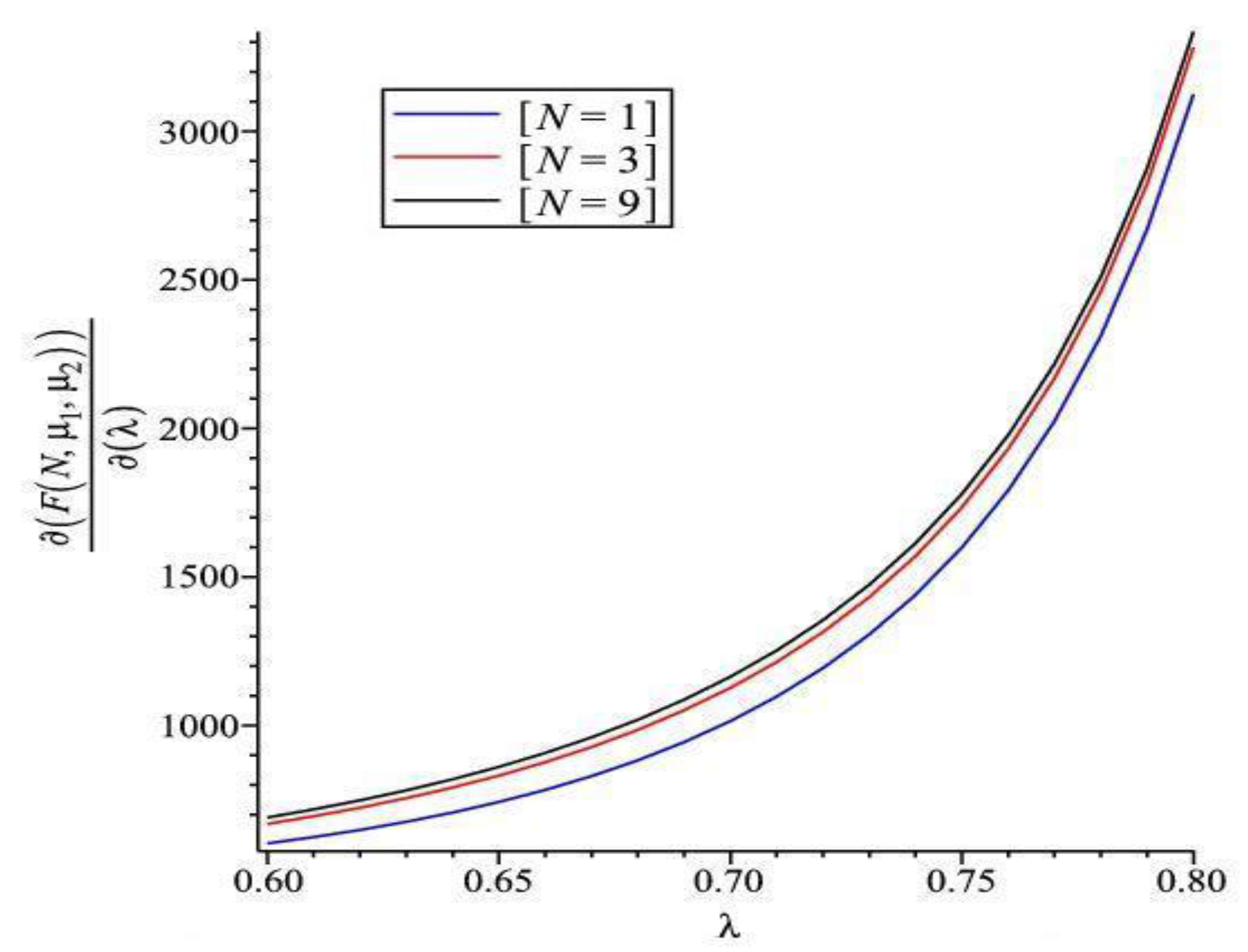
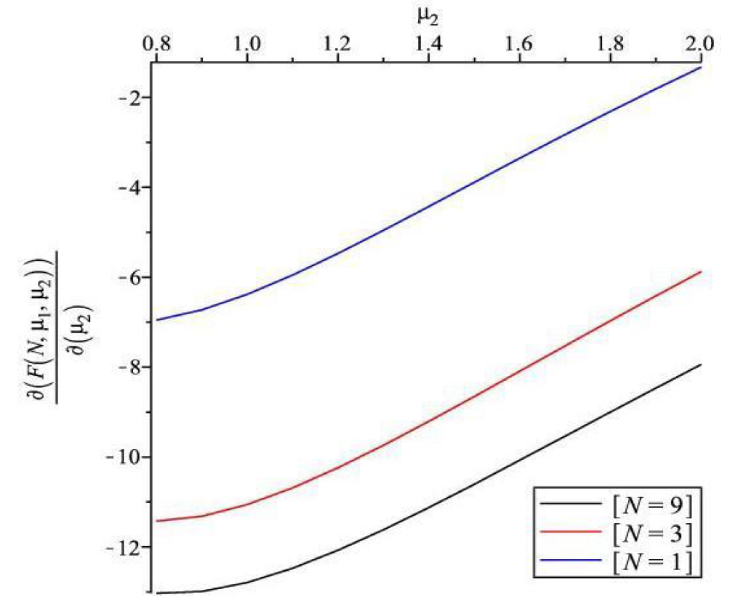
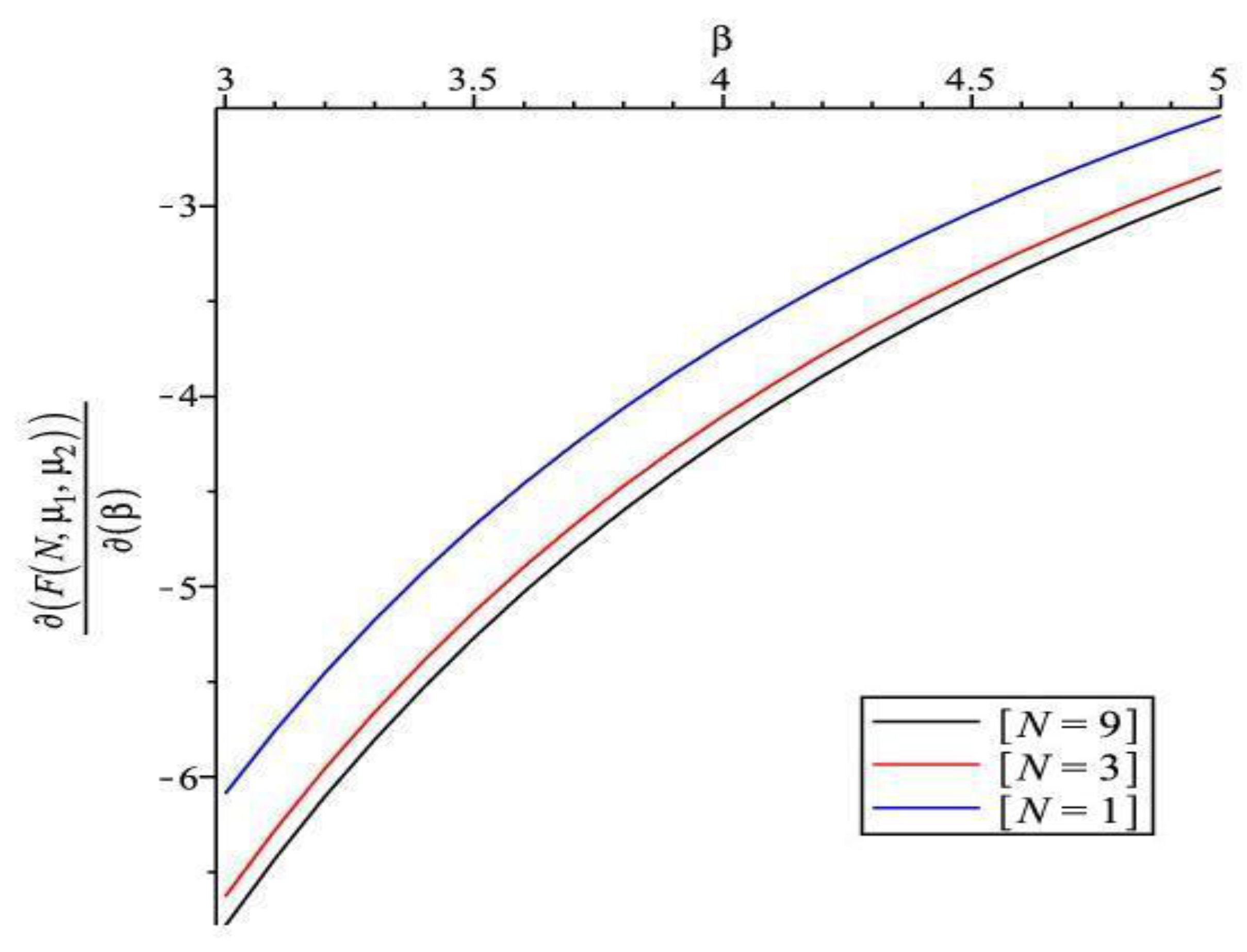
5.4. Sensitivity Analysis for the Expected Cost Function

In this section, we fulfill a sensitivity analysis for the cost function with respect to changes in designated values of the system parameters. To analyze the influences of various system parameters on the cost function, we use a graphical analysis of the following five cases. We fix the following cost parameters:

$$C_h=\text{\$}60,C_f=\text{\$}80,C_o=\text{\$}300,C_b=\text{\$}600,C_s=\text{\$}320,C_1=\text{\$}20,C_2=\text{\$}10$$

to study the listed below five cases:

• Case 1: ${\mu }_1=1.0$, ${\mu }_2=0.8$, $\alpha =0.2$, $\beta =3.0$; select different values of $N=$ 1, 3, 9, and vary $\lambda$ from 0.6 to 0.8.
• Case 2: $\lambda =0.6$, ${\mu }_2=0.8$, $\alpha =0.2$, $\beta =3.0$; choose different values of $N=$ 1, 3, 9, and vary ${\mu }_1$ from 1.0 to 2.0.
• Case 3: $\lambda =0.6$, ${\mu }_1=1.0$, $\alpha =0.2$, $\beta =3.0$; select different values of $N=$1, 3, 9, and vary ${\mu }_2$ from 0.8 to 2.0.
• Case 4: $\lambda =0.6$, ${\mu }_1=1.0$, ${\mu }_2=0.8$, $\beta =3.0$; select different values of $N=$ 1, 3, 9, and vary $\alpha$ from 0.2 to 0.5.
• Case 5: $\lambda =0.6$, ${\mu }_1=1.0$, ${\mu }_2=0.8$, $\alpha =0.2$; choose different values of $N=$ 1, 3, 9, and vary $\beta$ from 3.0 to 5.0.

Figure 4, Figure 5, Figure 6, Figure 7 and Figure 8 show the sensitivity performance of the expected cost with respect to $\lambda$, ${\mu }_1$, ${\mu }_2$, $\alpha$, and $\beta$ for various values of $N=$1, 3, 9. We should note that the sign of sensitivity reveals the monotonicity of the expected cost by changing the values of system parameters. Figure 4 reveals that (i) $\partial F/\partial \lambda$ is positive, which means that incremental change of $\lambda$ increases the expected cost; (ii) $\partial F/\partial \lambda$ increases as $\lambda$ increases for all $N$; and (iii) as $\lambda$ is fixed, $\partial F/\partial \lambda$ becomes larger as $N$ increases. It appears from Figure 5 that (i) $\partial F/\partial {\mu }_1$ is negative, which means that incremental change of ${\mu }_1$ decreases the expected cost; and (ii)$\partial F/\partial {\mu }_1$ increases as ${\mu }_1$ increases for all $N$. Figure 6 shows that (i) $\partial F/\partial {\mu }_2$ is negative, which means that incremental change of ${\mu }_2$ decreases the expected cost; (ii) $\partial F/\partial {\mu }_2$ increases as ${\mu }_2$ increases; and (iii) as ${\mu }_2$ is fixed, $\partial F/\partial {\mu }_2$ becomes larger as $N$ decreases. Moreover, $\partial F/\partial {\mu }_2$ has a smaller increasing shape than $\partial F/\partial {\mu }_1$. We observe from Figure 7 that (i) $\partial F/\partial \alpha$ is positive; (ii) $\partial F/\partial \alpha$ increases as $\alpha$ increases for all $N$; (iii) as $\alpha$ is fixed, $\partial F/\partial \alpha$ increases as $N$ increases. It can be seen in Figure 8 that (i) $\partial F/\partial \beta$ is negative; (ii) $\partial F/\partial \beta$ increases as $\beta$ increases; and (iii) as $\beta$ is fixed, $\partial F/\partial \beta$ decreases as $N$ increases.

6. Conclusions

This paper studied the N policy M/G/1 queue with working breakdowns. Steady-state probabilities were obtained by means of the supplementary variable and probability generating function techniques. The expected cost function per unit time was established to determine the joint optimal values of $(N,{\mu }_1,{\mu }_2)$ until the stability constraint is satisfied. More especially, an efficient and useful method (two-stage optimization method) was utilized to search the optimal joint values of $(N,{\mu }_1,{\mu }_2)$ that minimize the cost function. Sensitivity analysis of the cost function has been performed for specific values of the system parameters $\lambda$, ${\mu }_1$, ${\mu }_2$, $\alpha$, and $\beta$, as well as various values of $N$.

References

1. Yadin, M.; Naor, P. Queueing systems with a removable service station. Oper. Res. Quar. 1963, 14, 393–405. [Google Scholar] [CrossRef]
2. Jayachitra, P.; Albert, A.J. Recent developments in queueing models under N-policy: A short survey. Int. J. Math. Arch. 2014, 5, 227–233. [Google Scholar]
3. Kalidass, K.; Kasturi, R. A queue with working breakdowns. Comput. Ind. Eng. 2012, 63, 779–783. [Google Scholar] [CrossRef]
4. Liou, C.-D. Markovian queue optimisation analysis with an unreliable server subject to working breakdowns and impatient customers. Int. J. Syst. Sci. 2015, 46, 2165–2182. [Google Scholar] [CrossRef]
5. Kim, B.K.; Lee, D.H. The M/G/1 queue with disasters and working breakdowns. Appl. Math. Modell. 2014, 38, 1788–1798. [Google Scholar] [CrossRef]
6. Wang, K.-H.; Ke, J.-C. Control policies of an M/G/1 queueing system with a removable and non-reliable server. Inter. Trans. Oper. Res. 2002, 9, 195–212. [Google Scholar] [CrossRef]
7. Wang, K.-H. Optimal operation of a Markovian queueing system with a removable and non-reliable server. Microelectron. Reliab. 1995, 35, 1131–1136. [Google Scholar] [CrossRef]
8. Ke, J.-C.; Pearn, W.L. Optimal management policy for heterogeneous arrival queueing systems with server breakdowns and vacations. Qual. Tech. Quant. Manag. 2004, 1, 149–162. [Google Scholar] [CrossRef]
9. Wang, K.-H.; Wang, T.-Y.; Pearn, W.L. Maximum entropy analysis to the N policy M/G/1 queueing system with server breakdowns and general startup times. Appl. Math. Comput. 2005, 165, 45–61. [Google Scholar] [CrossRef]
10. Ke, J.-C.; Lin, C.-H. Maximum entropy approach for batch-arrival queue under N policy with an un-reliable server and single vacation. J. Comput. Appl. Math. 2008, 221, 1–15. [Google Scholar] [CrossRef] [Green Version]
11. Wang, K.-H.; Wang, T.-Y.; Pearn, W.L. Optimal control of the N policy M/G/1 queueing system with server breakdowns and general startup times. Appl. Math. Modell. 2007, 31, 2199–2212. [Google Scholar] [CrossRef]
12. Jain, M.; Bhargava, C. N-policy machine repair system with mixed standbys and unreliable server. Qual. Tech. Quant. Manag. 2009, 6, 171–184. [Google Scholar] [CrossRef]
13. Vemuri, V.K.; Boppana, V.S.N.H.P.; Kotagiri, C.; Bethapudi, R.T. Optimal strategy analysis of an N-policy two-phase MX/M/1 queueing system with server startup and breakdowns. OPSEARCH 2011, 48, 109–122. [Google Scholar] [CrossRef]
14. Singh, C.J.; Jain, M.; Kumar, B. Analysis of queue with two phases of service and m phases of repair for server breakdown under N-policy. Int. J. Serv. Oper. Manag. 2013, 16, 373–406. [Google Scholar] [CrossRef]
15. Yang, D.-Y.; Ke, J.-C. Cost optimization of a repairable M/G/1 queue with a randomized policy and single vacation. Appl. Math. Modell. 2014, 38, 5113–5125. [Google Scholar] [CrossRef]
16. Chen, W.L.; Wang, K.-H. Reliability analysis of a retrial machine repair problem with warm standbys and a single server with N-policy. Reliab. Eng. Syst. Saf. 2018, 180, 476–486. [Google Scholar] [CrossRef]
17. Cox, D.R. The analysis of non-Markovian stochastic processes by the inclusion of supplementary variables. Proc. Camb. Philos. Soc. 1955, 51, 433–441. [Google Scholar] [CrossRef]
18. Nocedal, J.; Wright, S.J. Numerical Optimization; Springer Series in Operations Research; Springer: New York, NY, USA, 1999. [Google Scholar]
Figure 1. A cloud data center provides a platform as a service (PaaS) via CloudStack.VM, virtual machine; OSD, object store daemon; MON, monitor.
Symmetry 12 00583 g001
Figure 2. Plot of F ( N , μ 1 , μ 2 ) for different values of λ .
Symmetry 12 00583 g002
Figure 3. Plot of F ( N , μ 1 , μ 2 ) for N = 2, λ = 0.4 , α = 0.2 , β = 0.3 .
Symmetry 12 00583 g003
Figure 4. Sensitivity analysis of F with respect to λ for different N ( μ 1 = 1.0 , μ 2 = 0.8 , α = 0.2 , β = 3.0 ).
Symmetry 12 00583 g004
Figure 5. Sensitivity analysis of F with respect to μ 1 for different N ( λ = 0.6 , μ 2 = 0.8 , α = 0.2 , β = 3.0 ).
Symmetry 12 00583 g005
Figure 6. Sensitivity analysis of F with respect to μ 2 for different N ( λ = 0.6 , μ 1 = 1.0 , α = 0.2 , β = 3.0 ).
Symmetry 12 00583 g006
Figure 7. Sensitivity analysis of F with respect to α for different N ( λ = 0.6 , μ 1 = 1.0 , μ 2 = 0.8 , β = 3.0 ).
Symmetry 12 00583 g007
Figure 8. Sensitivity analysis of F with respect to β for different N ( λ = 0.6 , μ 1 = 1.0 , μ 2 = 0.8 , α = 0.2 ).
Symmetry 12 00583 g008