Learning the Kinematics of a Manipulator Based on VQTAM

Abstract

The kinematics of a robotic manipulator is critical to the real-time performance and robustness of the robot control system. This paper proposes a surrogate model of inverse kinematics for the serial six-degree of freedom (6-DOF) robotic manipulator, based on its kinematics symmetry. Herein, the inverse kinematics model is derived via the training of the Vector-Quantified Temporal Associative Memory (VQTAM) network, which originates from Self-Organized Mapping (SOM). During the processes of training, testing, and estimating of this neural network, a priority K-means tree search algorithm is utilized, thus improving the training efficacy. Furthermore, Local Linear Regression (LLR), Local Weighted Linear Regression (LWR), and Local Linear Embedding (LLE) algorithms are, respectively, combined with VQTAM to obtain three improvement algorithms, all of which aim to further optimize the prediction accuracy of the networks for subsequent comparison and selection. To speed up the solving of the least squared equation, which is common among the three algorithms, Singular Value Decomposition (SVD) is introduced. Finally, data from forward kinematics, in the form of the exponential product of a motion screw, are obtained, and are used for the construction and validation of the VQTAM neural network. Our results show that the prediction effect of the LLE algorithm is better than others, and that the LLE algorithm is a potential surrogate model to estimate the output of inverse kinematics.

1. Introduction

The robotic manipulator has been commonly used in various fields. Robot control is critical for high-speed and high-precision robot motion, and it is based on the kinematics of robots. Kinematics includes two aspects: forward kinematics and inverse kinematics. Inverse kinematics describes the mapping from the state of effector to the state of actuator [1]. The key to kinematics is establishing the mapping relationship of the manipulator. For the serial robot, the input is the rotation angle of each joint, and the output is the pose of the end effector.

Generally, the inverse kinematics analysis of serial robots requires highly complex calculations, which affect the response speed and work efficiency of the robot controller. The same problem also exists in the forward kinematics of parallel robots. Three types of methods are typically used for the inverse kinematics of serial robots: geometric [2,3,4], algebraic [5,6,7], and iterative algorithms [8,9,10,11,12]. However, algebraic methods cannot always derive a closed-form solution. In addition, the use of geometric methods is limited by the precondition, and the initial position influences the convergence speed of iterative algorithms. Using these three methods, the inverse kinematics of the robot cannot be obtained quickly and effectively [1]. Therefore, much research is focused on how to simplify the solution of robot kinematics. Intelligent algorithms and machine learning are combined in solving the kinematics of the robot. Simpler mapping models of the kinematic input and output are established to replace the complex analytical solution. Robot kinematics has symmetry, meaning that the input and output of forward kinematics are the output and input of inverse kinematics, respectively. The manipulator’s state of forward kinematics and inverse kinematics correspond one by one. According to this symmetry, the forward kinematics of the robotic manipulator can be used to generate sample data to train its inverse kinematics model. Hargis, B.E. et al. [13] trained an Artificial Neural Network (ANN) to obtain the inverse kinematics solution. Lou, Y. F. et al. [14] used a hybrid ANN to solve the inverse kinematics and realized the path control of a two-degree of freedom (2-DOF) manipulator. Akanshu Mahajan et al. [15] established an unsupervised learning algorithm based on a neural network, which approximately replaced the inverse kinematics model of the 2-DOF serial robot. Ben Kenwright [16] solved inverse kinematic problems by combining an ANN and a differential evolutionary algorithm. Koji Kinoshita [17] regarded the inverse kinematics of a 3-DOF manipulator as an optimization problem, and solved it using a Particle Swarm Optimization (PSO) algorithm. Rui Ting, Zhu et al. [18] proposed a method based on PSO to obtain an optimal solution using kinematic equations directly. Other agent models or intelligent optimization algorithms, such as evolutionary fuzzy extreme learning machine, support vector regression, RBF (Radial Basis Function) networks, Kohonen self-organizing map, modular neural network systems, sequential mutation genetic algorithms, etc., have been applied in robot kinematics [1,19,20,21,22,23,24,25]. When the DOF of the robotic manipulator is increased, the corresponding calculation amount increases in a geometric series. Therefore, the existing methods are not suitable for the inverse kinematics of a 6-DOF robotic manipulator. At the same time, the existing achievements are mostly based on the neural network model. The selection of hyperparameters of the neural network has a great impact on the prediction accuracy. Therefore, adjusting the parameters is time-consuming. Another problem of the neural network model is that it easily converges to the local optimum in the training process.

Robot kinematics can be regarded as a Nonlinear Autoregressive Model with Exogenous Input (NARX). In [26], the forward kinematics of parallel manipulators is solved by combining the wavelet network and NARX method. However, the validity of this method still relies on parameter initialization and the backpropagation learning process.

In [27], a self-organizing map structure was proposed, namely, the Vector-Quantified Temporal Associative Memory (VQTAM). Barreto, G. D. and Araujo, A. F. R. simulated a one-dimensional network, which was compared with the multilayer perceptron (MLP) and RBF networks. Furthermore, a VQTAM network with higher dimensions may behave better. Thus, in this paper, we train two-dimensional networks to research their performance. The VQTAM algorithm does not depend on the adjustment of hyperparameters, but on Self-Organized Mapping (SOM) to achieve topology preservation [27]. As an extension of SOM, it can be applied to the mapping between two spaces. The mathematical foundation of VQTAM is nonlinear manifold embedding. This method is suitable for time series modeling and the prediction of nonlinear systems. Depending on the self-organizing mapping structure, the discrete mapping relationship can effectively realize output estimation according to exogenous input [27,28,29]. Because spaces of VQTAM are discrete, a network with a large number of neurons is needed to achieve high-precision prediction. To improve the computational efficiency, it is necessary to reduce the number of VQTAM neurons. Based on VQTAM and Local Linear Embedding (LLE), the input is locally linearized in the neighborhood. Improved local linear algorithms of VQTAM are proposed to solve the inverse kinematics of a 6-DOF robot efficiently and accurately.

The paper discusses the complexity of the inverse kinematics solution when applied to serial manipulators. Meanwhile, the kinematics of parallel manipulators would be more complex, and it could also be effectively solved by the methods provided in this paper. This part of the work will be covered in the authors’ future research.

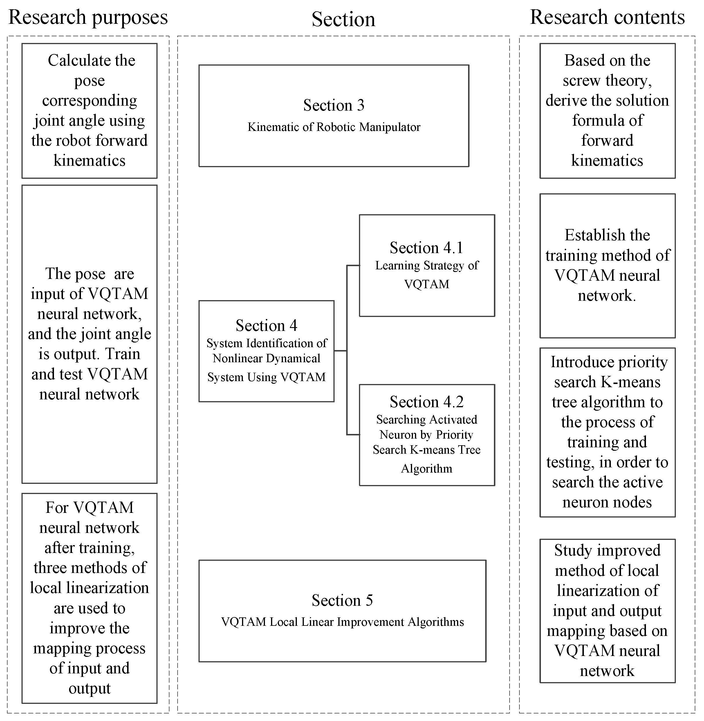
2. Research Methodology

A robotic manipulator is a typical open-loop mechanism. Its forward kinematics can be achieved by coordinate transformation, D-H parameters, screw theory, and other mathematical tools. The result can be obtained quickly. However, the inverse solution of serial robots is very complex. The robotic manipulator is a nonlinear system. Generally, solving the inverse kinematics and dynamics accurately and conveniently is difficult.

Thus, the poses corresponding to different joint angles can be obtained using forward kinematics. The data obtained can be used to train the surrogate model for inverse kinematics based on its symmetry. In this paper, a VQTAM neural network is introduced to replace the complex calculation of inverse kinematics. The research content and structure of this paper are shown in Figure 1.

In Section 3, the forward kinematics is studied. Data for training are sampled from forward kinematics, meaning that each pose of the end effector corresponds to a group of joint angles.

In Section 4, the nonlinear system identification method based on VQTAM is studied, and the training method of the VQTAM neural network is established. In the process of VQTAM training and testing, it is critical to search activated neuron nodes. Moreover, the priority search K-means tree algorithm is introduced for this step.

In Section 5, the improved method of local linearization for the mapping process based on the VQTAM neural network is studied.

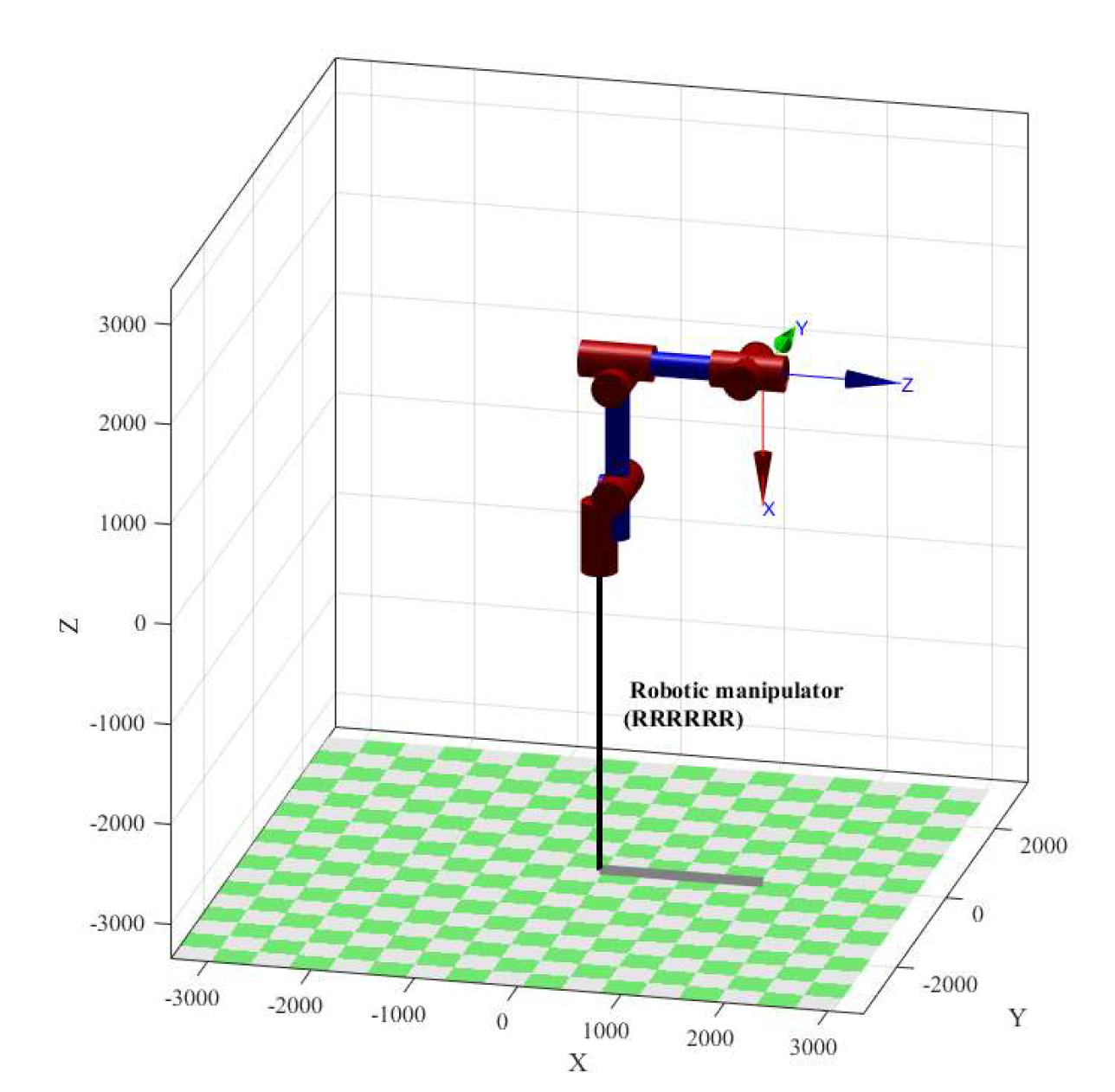
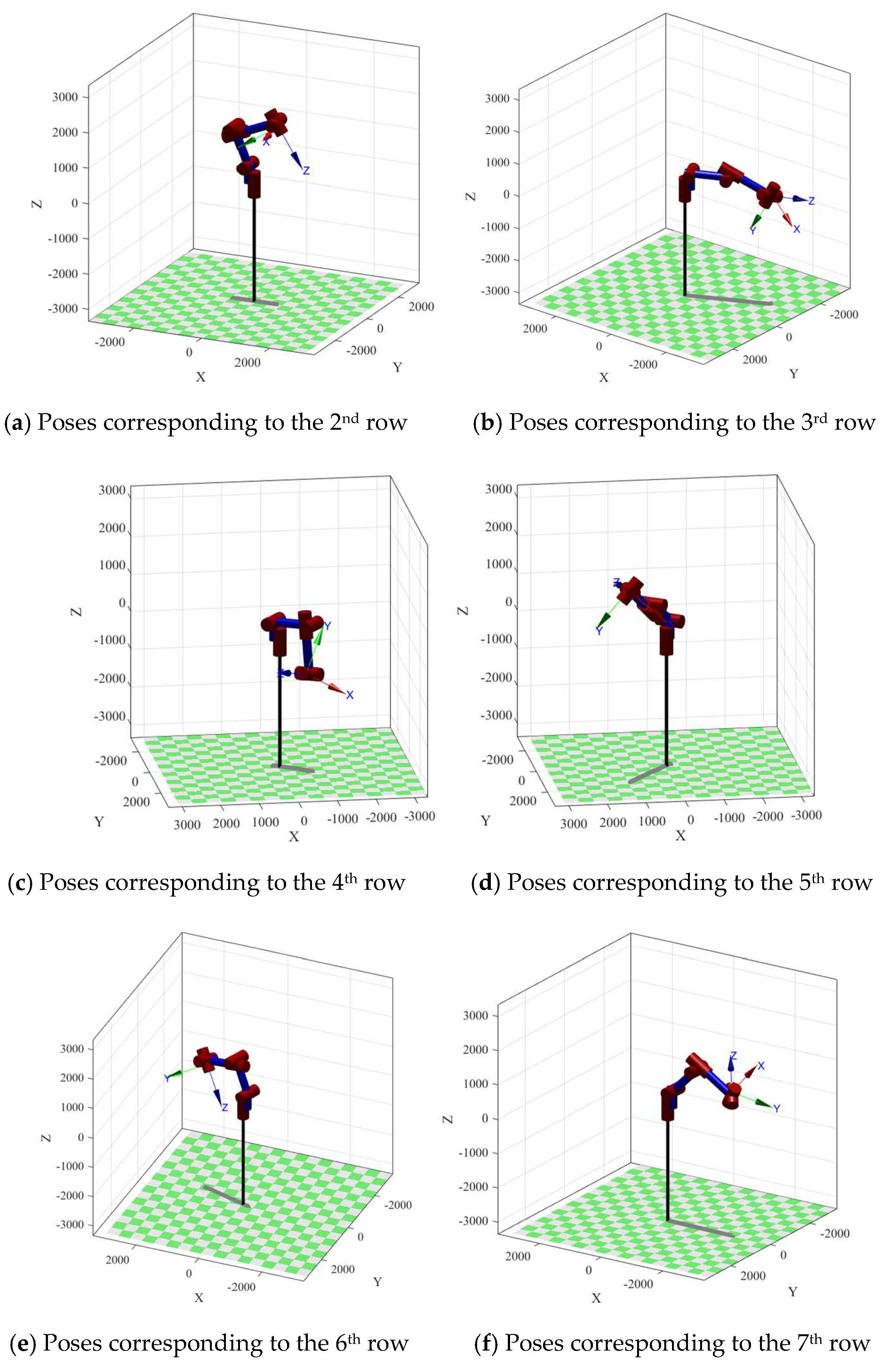
3. Kinematics of the Robotic Manipulator

In screw theory, any motion of a rigid body can be decomposed into rotational motion around a straight line and translational motion along the line. That is to say, the motion of a rigid body can be regarded as spiral motion.

Using screw theory has the following advantages in rigid body kinematics [5,30,31]:

(1)

The 6-DOF parameter is used to describe the pose relationship between two adjacent coordinate systems completely, thus avoiding the lack of completeness in the D-H model.

(2)

The global coordinate system is used to describe the motion state of a rigid body, which overcomes the singularity of the D-H model.

(3)

The motion characteristics of rigid bodies can be clearly described from a global perspective, thus simplifying the analysis of complex mechanisms and avoiding the abstraction of mathematical symbols.

To sum up, the advantages of screw include a clear geometric concept, clear physical meaning, simple expression, and efficient algebraic operation in the kinematics of the robotic manipulator.

According to Chasles’ theorem, the spiral motion of a rigid body can be expressed in the form of exponential coordinates of the screw. For the 6-DOF robotic manipulator (RRRRRR type) shown in Figure 2, the relative inertial coordinate system of each joint is established according to screw theory, as shown in Equation (1).

$$\begin{array}{c}{\mathit{\omega }}_1=\left[\begin{array}{c}0\\ 0\\ 1\end{array}\right]{\mathit{\omega }}_2=\left[\begin{array}{c}1\\ 0\\ 0\end{array}\right]{\mathit{\omega }}_3=\left[\begin{array}{c}0\\ 1\\ 0\end{array}\right]\\ {\mathit{\omega }}_4=\left[\begin{array}{c}1\\ 0\\ 0\end{array}\right]{\mathit{\omega }}_5=\left[\begin{array}{c}0\\ 1\\ 0\end{array}\right]{\mathit{\omega }}_6=\left[\begin{array}{c}1\\ 0\\ 0\end{array}\right]\end{array}$$

(1)

The coordinates of the points on the axes of each joint are shown in Equation (2).

$$\begin{array}{c}{\mathit{r}}_1=\left[\begin{array}{c}0\\ 0\\ 0\end{array}\right]{\mathit{r}}_2=\left[\begin{array}{c}{x}_2\\ 0\\ z_2\end{array}\right]{\mathit{r}}_3=\left[\begin{array}{c}{x}_3\\ 0\\ z_3\end{array}\right]\\ {\mathit{r}}_4=\left[\begin{array}{c}{x}_4\\ 0\\ z_4\end{array}\right]{\mathit{r}}_5=\left[\begin{array}{c}{x}_5\\ 0\\ z_5\end{array}\right]{\mathit{r}}_6=\left[\begin{array}{c}{x}_6\\ 0\\ z_6\end{array}\right]\end{array}$$

(2)

Then, the unit screw of each joint can be obtained as shown in Equation (3).

$$\begin{gathered} {\mathit{\xi }}_1=\left[\begin{array}{c}0\\ 0\\ 1\\ 0\\ 0\\ 0\end{array}\right]{\mathit{\xi }}_2=\left[\begin{array}{c}1\\ 0\\ 0\\ 0\\ -z_2\\ 0\end{array}\right]{\mathit{\xi }}_3=\left[\begin{array}{c}0\\ 1\\ 0\\ z_3\\ 0\\ -x_3\end{array}\right] \\ {\mathit{\xi }}_4=\left[\begin{array}{c}1\\ 0\\ 0\\ 0\\ -z_4\\ 0\end{array}\right]{\mathit{\xi }}_5=\left[\begin{array}{c}0\\ 1\\ 0\\ z_5\\ 0\\ -x_5\end{array}\right]{\mathit{\xi }}_6=\left[\begin{array}{c}1\\ 0\\ 0\\ 0\\ -z_6\\ 0\end{array}\right] \end{gathered}$$

(3)

ω_i can be mapped to the rigid body rotation transformation matrix to describe the rigid body rotation transformation in three-dimensional space, as shown in Equation (4). v_i is the vector comprising the third, fourth, and fifth components of the screw, ξ_i.

$${\mathit{\omega }}_i=\left[\begin{array}{c}{\omega }_i^1\\ {\omega }_i^2\\ {\omega }_i^3\end{array}\right]\mapsto {\widehat{\mathit{\omega }}}_i=\left[\begin{array}{ccc}0& -{\omega }_i^3& {\omega }_i^2\\ {\omega }_i^3& 0& -{\omega }_i^1\\ -{\omega }_i^2& {\omega }_i^1& 0\end{array}\right]$$

(4)

ξ_i can be mapped to a rigid body transformation matrix, describing the rigid body transformation in three-dimensional space, as shown in Equation (5).

$${\mathit{\xi }}_i={\left[{\mathit{\omega }}_i^T;{\mathit{v}}_i^T\right]}^T\mapsto {\widehat{\mathit{\xi }}}_i=\left[\begin{array}{cc}{\widehat{\mathit{\omega }}}_i& {\mathit{v}}_i\\ \mathbf{0}& 0\end{array}\right]$$

(5)

As a special Euclidean group SE(3), the rigid body transformation matrix in three-dimensional space can be regarded as a six-dimensional manifold, and the points on the manifold correspond to the rigid body transformation. SE(3) comprises all possible rigid body motion mappings. Then, ${\widehat{\mathit{\xi }}}_i$ is the Lie algebra se(3) of SE(3). According to the isomorphism relation shown in Equation (6), the mapping relation between the Plucker coordinate form and matrix ${\widehat{\mathit{\xi }}}_i$ can be defined and expressed using operators ∨ and ∧, as shown in Equations (7) and (8).

$${\widehat{\mathit{\xi }}}_i=\left[\begin{array}{cc}{\widehat{\mathit{\omega }}}_i& {\mathit{v}}_i\\ 0& 0\end{array}\right]\in se(3)\mapsto {\left[{\mathit{\omega }}_i^T;{\mathit{v}}_i^T\right]}^T\in {\mathrm{ℝ}}^6$$

(6)

$${\left[\begin{array}{cc}{\widehat{\mathit{\omega }}}_i& {\mathit{v}}_i\\ 0& 0\end{array}\right]}^{\vee }=\left(\begin{array}{c}{\mathit{\omega }}_i\\ {\mathit{v}}_i\end{array}\right)$$

(7)

$${\left(\begin{array}{c}{\mathit{\omega }}_i\\ {\mathit{v}}_i\end{array}\right)}^{\wedge }=\left[\begin{array}{cc}{\widehat{\mathit{\omega }}}_i& {\mathit{v}}_i\\ 0& 0\end{array}\right]$$

(8)

The helical motion of a rigid body g ∈ se(3) is expressed in the form of exponential coordinates of the motion screw, as shown in Equation (9) [30,31].

$${\mathit{g}}_i=e^{{\widehat{\mathit{\xi }}}_{\mathit{i}}{\theta }_i}=\{\begin{array}{c}\left[\begin{array}{cc}{e}^{{\widehat{\mathit{\omega }}}_i{\theta }_i}& (\mathit{I}-e^{{\widehat{\mathit{\omega }}}_i{\theta }_i})({\mathit{\omega }}_i\times {\mathit{v}}_i)+{\theta }_i{\mathit{\omega }}_i{\omega }_i^T{\mathit{v}}_i\\ 0& 1\end{array}\right],{\mathit{\omega }}_i\ne 0\\ \left[\begin{array}{cc}I& {\theta }_i{\mathit{v}}_i\\ 0& 1\end{array}\right],{\mathit{\omega }}_i=0\end{array}$$

(9)

Combining the motion of each joint, the exponential product equation of the forward kinematics of the robot is obtained, as shown in Equation (10) [30,31].

$$\begin{gathered} {\mathit{g}}_{st}(\mathit{\theta })=e^{e^{{\widehat{\mathit{\xi }}}_1{\theta }_1}}{e}^{e^{{\widehat{\mathit{\xi }}}_2{\theta }_2}}\dots e^{e^{{\widehat{\mathit{\xi }}}_6{\theta }_6}}{\mathit{g}}_{st}(0) \\ \mathit{\theta }=\left[{\theta }_1,{\theta }_2,{\theta }_3,{\theta }_4,{\theta }_5,{\theta }_6\right] \end{gathered}$$

(10)

g_st(0) is the pose in the initial state, and g_st(θ) is the pose of the manipulator, where θ is the angle vector of each joint relative to the initial state. Given the joint screw and initial pose, the forward kinematics solution of the robotic manipulator can be obtained.

The joint screw parameters of the robotic manipulator are given in

Table 1. Joint screw parameters.

parameter	x2 (mm)	x3 (mm)	x4 (mm)	x5 (mm)	x6 (mm)
value	175	175	175	1445	1445
parameter	z2 (mm)	z3 (mm)	z4 (mm)	z5 (mm)	z6 (mm)
value	495	1590	1765	1765	1765

. The pose shown in Figure 1 is determined to be the initial pose. Poses corresponding to different joint rotation angles can be obtained by Equation (10). Some data for computation validation are shown in

Table 2. Poses corresponding to different joint rotation angles.

θ						gst(θ)
θ1	θ2	θ3	θ4	θ5	θ6	x (mm)	y (mm)	z(mm)	u	v	w
0	0	0	0	0	0	1580	0	1765	−2.81	−1.57	2.81
−3.14	0.39	−3.14	0.03	−1.41	−4.81	717.58	9.07	1715.51	−1.44	−0.54	30.09
−2.71	1.58	−1.11	7.78	0.81	3.25	−2292.10	−1151.06	23.08	2.63	0.24	−1.95
−0.63	−1.53	−3.1	−1.46	−1.82	−5.04	−597.84	594.06	−706.84	−2.67	−0.73	1.24
−2.24	−0.95	−1.55	7.43	2.22	6.30	1152.39	1311.719	1743.21	2.40	−0.15	−1.67
2.81	−0.42	−2.98	−2.90	2.01	6.95	1304.39	−420.67	912.84	2.02	0.54	2.64
3.12	0.79	−0.24	−7.64	−2.34	−7.61	−2057.54	−44.10	822.60	−2.44	−0.52	−0.97

and Figure 3, which were drawn using the robotics MATLAB toolbox by Peter Corke. In Table 2, (x,y,z) represents the position coordinate of the end actuator, and (u,v,w) is the attitude in Euler angle in radians.

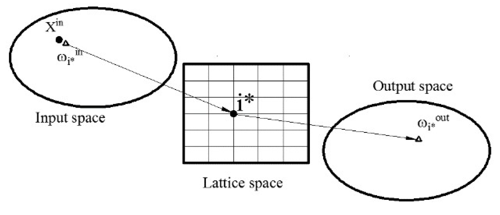
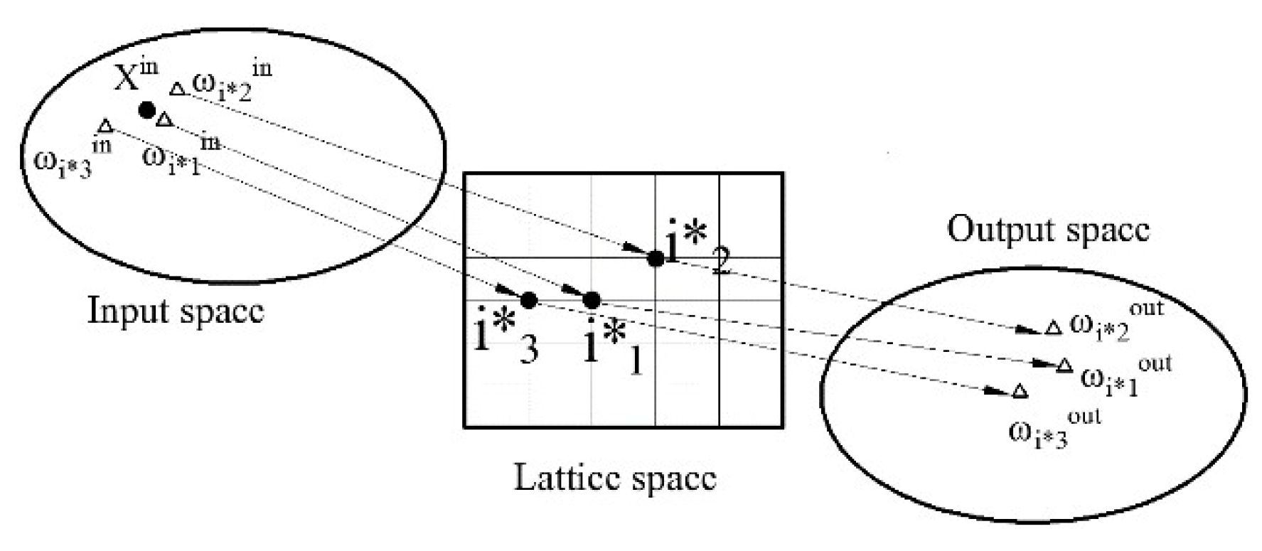
4. System Identification of a Nonlinear Dynamical System Using VQTAM

The inverse kinematics of the robotic manipulator aims at solving the corresponding joint rotation once given the pose and initial pose of the manipulator. The joint rotation angle is regarded as output Q and the pose as input p. The inverse kinematics problem of the robot can be transformed into the identification problem of a nonlinear dynamic system. The time-discrete difference equation is established as shown in Equation (11) [27,29]. Q(t) = θ(t) is the joint rotation angle variable of the manipulator. p(t) = [x(t),y(t),z(t);u(t),v(t),w(t)] is the pose of the manipulator at t time. It is expressed by the position coordinates combined with the Euler angle. f(∙) represents a nonlinear function reflecting the characteristics of the system. The output Q at t + 1 is determined by the previous n_q outputs and n_p inputs.

The purpose of inverse kinematics is to find the mapping function f(∙) between the input and output. As a complex nonlinear problem, on the premise of ensuring the accuracy, simplifying the model can improve efficiency and ensure real-time performance in engineering applications.

$$\mathit{Q}(t+1)=f[\mathit{Q}(t),\dots ,\mathit{Q}(t-n_q+1);\mathit{p}(t),\dots ,\mathit{p}(t-n_u+1)]$$

(11)

$${\mathit{X}}^{in}=[\mathit{Q}(t),\dots ,\mathit{Q}(t-n_q+1);\mathit{p}(t),\dots ,\mathit{p}(t-n_u+1)]$$

(12)

$${\mathit{X}}^{out}=[\mathit{Q}(t+1)]$$

(13)

VQTAM is a variant of SOM, which can be used to realize nonlinear mapping. The concept of nonlinear manifold embedding can be used to establish the nonlinear mapping. SOM is realized through competition and cooperation among feature neurons. In the mapping process, different neurons are activated for different inputs, and the activated neurons affect the output together with the neurons in their neighborhood. Therefore, time series data can be constructed as training samples of VQTAM.

VQTAM adopts training samples to build a topological structure embedded in multidimensional data space, which can construct the mapping relationship between multidimensional input vectors and multidimensional output vectors. VQTAM consists of three layers: input space ωⁱⁿ, output space ω^out, and lattice space. The establishment of the mapping process is shown in Figure 4. The definitions of Xⁱⁿ and X^out are shown in Equations (12) and (13), respectively.

The input space and output space are composed of the weight vectors ω_iⁱⁿ and ω_i^out, respectively, where i is the index of the neuron in lattice space that reflects the location of the neuron in the lattice topology structure. Weight vectors ω_iⁱⁿ and ω_i^out have mapping relationships with neurons in lattice space. ω_iⁱⁿ and ω_i^out have the same dimensions as Xⁱⁿ and X^out, respectively. In the mapping process of VQTAM, the nearest weight vector ω_i*ⁱⁿ to Xⁱⁿ is found in the input space, which corresponds to the activated neuron in the lattice space. In this process, the Euclidean distance is used to measure the distance between two vectors. The definition of i* is shown in Equation (14), where A is the collection of all neuron indexes in lattice space [27].

$$i*=\underset{i\in A}{\arg \min }\left\{\Vert {\mathit{X}}^{in}-{\mathit{\omega }}_i^{in}\Vert \right\}$$

(14)

ω_i*^out is obtained according to the neuron index i*, and the output X^out is estimated, as shown in Equation (15).

$${\widehat{\mathit{X}}}^{out}={\mathit{\omega }}_{i*}^{out}$$

(15)

4.1. Learning Strategy of VQTAM

The main parameters of VQTAM are neuron weight vectors ω_iⁱⁿ and ω_i^out, and lattice topology. The initial lattice topology structure can be determined as a hyperparameter before training, so the learning strategy mainly aims at updating the weight vectors ω_iⁱⁿ and ω_i^out in the training process.

There is competition and cooperation among neurons in SOM. Different neurons and their neighborhoods are activated by inputting to participate in the learning process, and the weight vectors ω_iⁱⁿ and ω_i^out are updated. The index search of the active neurons in the lattice space is consistent with Equation (14).

To improve the convergence rate in the learning process, the influence range parameters σ(t) of the activation neuron and the learning speed α(t) decrease exponentially with the learning epoch, as shown in Equations (16) and (17).

$$\alpha (t)={\alpha }_0{({\alpha }_T/{\alpha }_0)}^{t/T}$$

(16)

$$\sigma (t)={\sigma }_0{({\sigma }_T/{\sigma }_0)}^{t/T}$$

(17)

where t is the current learning epoch, T is the total learning epoch. α₀, σ₀ are the initial values, and α_T, σ_T are the parameter values of the T training epoch.

The Gauss neighborhood function is used to determine the effect of input on the neighbors of the activated neuron, as shown in Equation (18) [27,28,29].

$$h(i*,i;t)=\exp \left(\frac{-{\Vert i(t)-i*(t)\Vert }^2}{{\sigma }^2(t)}\right)$$

(18)

Complete the updates of ω_iⁱⁿ and ω_i^out, respectively, as shown in Equations (19) and (20).

$${\mathit{\omega }}_i^{in}\Leftarrow \alpha (t)h(i*,i;t)[{\mathit{X}}^{in}-{\mathit{\omega }}_i^{in}]$$

(19)

$${\mathit{\omega }}_i^{out}\Leftarrow \alpha (t)h(i*,i;t)[{\mathit{X}}^{out}-{\mathit{\omega }}_i^{out}]$$

(20)

To sum up, the VQTAM algorithm flow is as follows.

Algorithm 1: VQTAM Algorithm:

Begin

(training part)

1 Input: Xin and Xout in training set

2 Search activating neuron according to Xin

$i*=\underset{i\in A}{\arg \min }\left\{\Vert {\mathit{X}}^{in}-{\omega }_i^{in}\Vert \right\}$

3 Update the weight vector of the neuron

${\omega }_i^{in}\Leftarrow \alpha (t)h(i*,i;t)[X^{in}-{\omega }_i^{in}]$

${\omega }_i^{out}\Leftarrow \alpha (t)h(i*,i;t)[{\mathit{X}}^{out}-{\omega }_i^{out}]$

4 Continue execution until termination conditions are met

(testing part)

5 Input: Xtestin in testing set

6 Search activating neuron according to Xtestin

$i*=\underset{i\in A}{\arg \min }\left\{\Vert {\mathit{X}}_{test}^{in}-{\omega }_i^{in}\Vert \right\}$

7 Output:

${\widehat{\mathit{X}}}_{test}^{out}={\omega }_{i*}^{out}$

4.2. Searching the Activated Neuron by the Priority Search K-Means Tree Algorithm

During the training, testing, and estimation of VQTAM, the weight vector ω_i*ⁱⁿ to which Xⁱⁿ is nearest in the input space is searched, as shown in Equation (14). The search algorithm applied has a great impact on the efficiency of VQTAM. The global traversal method needs to find all the Euclidean distance from the weight vector ω_iⁱⁿ to the input Xⁱⁿ, and search the minimum value through traversal, which is inefficient. The K-Dtree algorithm can reduce the time complexity of searching, but for d-dimensional data, the time complexity of the K-Dtree data structure search is O(n^d/(d−1)). For a high-dimensional data search, especially when the data dimension d > 20, the K-Dtree data structure is inefficient. ω_iⁱⁿ is 30-dimensional. The searching efficiency is severely restricted. The search time complexity of the priority search k-means tree algorithm (PSKMT) is O(Ld logn/logK), where n is the amount of data in the data set, K is the number of nearest neighbors to be searched, and L is the maximum number of data retrieved in the search process. The priority search k-means tree algorithm is suitable for searching high-dimensional data.

The PSKMT algorithm divides the space into B different regions using the k-means clustering algorithm. Then, the points in each region are partitioned by the same operation until the number of data points in the region is no greater than K. In the process of searching, the idea of “divide and conquer” is used to find the nearest point in a smaller area and reduce the amount of data to be searched, so as to improve the efficiency.

The algorithm used for establishing a priority search K-means tree data structure is as follows.

Algorithm 2: K-means tree data structure building Algorithm [32]:

Begin

1 Input: weight vector ωiin as search data set D, branch parameter B, maximum iteration number Imax, center selection algorithm using Calg

2 Compare size |D| of data set D with branch parameter B

3 If |D|<B: Create leaf nodes from data sets

4 else, P ← uses Calg algorithm to select B points from data set D

5 start loop:

6 C ← Clustering Data in D Centered on P

7 Pnew ← Finding the Mean Value of Group C Data after Clustering

8 if P = Pnew, Pnew is the non-leaf node, and terminate the loop

9 These processes are executed on the sub-regions C until all leaf nodes are created

10 Output: the entire K-means tree data structure

In the establishment of the K-means tree, the algorithm C_alg is used to select B points from data set D that can be chosen from the random selection, Gonzale, and K-Means++ algorithms. The specific algorithm has little effect on data structure establishment. Generally, the random algorithm is recommended [16].

In the built K-means tree, leaf nodes are the data points in the original data set, and non-leaf nodes are the central points of the regions after segmentation. The search process can only be executed in a few areas, thus avoiding the global search of data sets. The K-means tree data structure is searched from the root node. Sub-nodes are sorted according to the distance between the clustering center and the query data points. The nearest sub-nodes are searched in advance. The priority K-means tree search algorithm is as follows.

Algorithm 3: PSKMT Algorithm [32]:

Input: K-means tree, query data Q (Xin), the nearest neighbor number K, the maximum number of search data L Initialize a stack and place the root node in the stack Starts loop. The condition for termination is that the stack is not empty and the amount of retrieved data |P| is less than L: If the top node of the stack is a leaf node, add it to the retrieved data array P Otherwise, the top node goes out of the stack, reads the sub-nodes, sorts them according to the distance between the clustering center and the query data points, and pushes them into the stack. Loop terminated Output: K data nearest to query data Q in retrieval data array P.

5. VQTAM Local Linear Improvement Algorithms

The VQTAM algorithm is used to quantify the input space ωⁱⁿ and output space ω^out. The neurons in ωⁱⁿ and ω^out correspond to each other through mapping relations. The input Xⁱⁿ is approximated to the nearest neuron ω_i*ⁱⁿ in estimation. The accuracy of the estimation results can be guaranteed when the number of neurons is large enough. However, the increase in number is followed by an increase in network size and a decrease in computing efficiency. Thus, local linearization of the activated node is used, which can balance the number of neurons and prediction accuracy. Based on local linearization, three improved algorithms for VQTAM are proposed: Local Linear Regression (LLR), Local Weighted Linear Regression (LWR), and LLE. The inverse kinematics can be further optimized, ensuring the computational efficiency.

Local linearization is performed in VQTAM networks. The K-means tree algorithm is used to search the nearest n data points ω_i*nⁱⁿ and the corresponding output data ω_i*n^out are mapped, as shown in Figure 5.

5.1. Improvement Algorithm of VQTAM with LLR

It is assumed that the relationship between the local input and output can be expressed linearly, so LLR can be performed as shown in Equation (21).

$$\mathit{Y}\mathit{B}=\mathit{Z}$$

(21)

Y is the nearest neighborhood ω_i*nⁱⁿ of Xⁱⁿ, and Z is the corresponding data point ω_i*n^out, as shown in Equations (22) and (23).

$$\mathit{Y}=\left[\begin{array}{c}{\omega }_{i*1}^{in}\\ ⋮\\ {\omega }_{i*n}^{in}\end{array}\right]\in {\mathrm{ℝ}}^{n\times m}$$

(22)

$$\mathit{Z}=\left[\begin{array}{c}{\omega }_{i*1}^{out}\\ ⋮\\ {\omega }_{i*n}^{out}\end{array}\right]\in {\mathrm{ℝ}}^{n\times l}$$

(23)

The linear relationship between the local input and output can be obtained by solving B. Equation (21) is an overdetermined equation, which is generally treated as a least squares problem and solved by a generalized inverse matrix, as shown in Equation (24).

$$\mathit{B}={({\mathit{Y}}^T\mathit{Y})}^{-1}{\mathit{Y}}^T\mathit{Y}$$

(24)

Y^TY is an n-dimensional square matrix, and the calculation of the inverse operation is huge when the dimension increases. Meanwhile, Y^TY may be a singular matrix or ill-conditioned matrix, so finding the inverse matrix directly is difficult. Singular Value Decomposition (SVD) can be used to solve the least squares problem. Y can be decomposed as shown in Equation (25).

$$\begin{array}{l}SVD(\mathit{Y})=[\mathit{U}][\mathit{S}][{\mathit{V}}^T]\\ where\mathit{Y}\in {\mathrm{ℝ}}^{m\times m},\mathit{U}\in {\mathrm{ℝ}}^{m\times l},\mathit{V}\in {\mathrm{ℝ}}^{l\times l}\end{array}$$

(25)

The column vectors of U are the eigenvectors of YY^T; the column vectors of V^T are the eigenvectors of Y^TY.

$$\mathit{S}=\left[\begin{array}{c}\mathit{\Sigma }\\ 0\end{array}\right]$$

(26)

Σ is a diagonal matrix whose value is the singular value υ of matrix Y, i.e., the eigenvalue of YY^T is λ = υ², and U and V^T are the orthogonal matrix.

U can be disassembled as [U_n, U_m-n]. For the least squares problem as shown in Equation (21), the solution obtained by SVD is shown in Equation (27).

$$\mathit{B}=\mathit{V}{\mathit{\Sigma }}^{-1}{\mathit{U}}_n^T\mathit{Z}$$

(27)

The input Xⁱⁿ is used to estimate the output, as shown in Equation (28).

$${\widehat{\mathit{X}}}^{out}={\mathit{X}}^{in}\mathit{B}$$

(28)

5.2. Improvement Algorithm of VQTAM with LWR

Using the LLR algorithm, the impact of all neighbor points on the prediction results is consistent. Considering the different influences of neighbor points, a distance weight is added in the regression process. A local weight linear regression (LWR) is adopted. The cost function is defined as shown in Equation (29).

The weight w_k in Equation (29) is determined by the Gauss neighborhood function, as shown in Equation (30), where τ is the bandwidth parameter.

$$J(\mathit{\phi })={\displaystyle \sum _{k=1}^n{w}_k{\Vert {\mathit{\omega }}_{i*k}^{out}-{\mathit{\phi }}_k{\mathit{\omega }}_{i*k}^{in}\Vert }^2}$$

(29)

$$w_k=\exp (-\frac{{\Vert {\mathit{X}}^{in}-{\mathit{\omega }}_{i*k}^{in}\Vert }^2}{{\tau }^2})$$

(30)

The analytical solution of the cost function minimization is equivalent to the solution of the overdetermined equation shown in Equation (31).

$$\mathit{W}\mathit{Y}\phi =\mathit{W}\mathit{Z}$$

(31)

where W is an n-dimensional diagonal matrix, and the diagonal element is w_k.

The SVD for matrix WY is also used to solve the overdetermined equation.

$$SVD(\mathit{W}\mathit{Y})=[\mathit{U}\mathit{Y}][\mathit{S}][{\mathit{V}}^T]$$

(32)

$$\mathit{\phi }=\mathit{V}{\mathit{\Sigma }}^{-1}{\mathit{U}}_n^T\mathit{W}\mathit{Z}$$

(33)

5.3. Improvement Algorithm of VQTAM with LLE

It is assumed that an input datum can be represented by a linear combination of several samples in its neighborhood; that is, the input Xⁱⁿ to be predicted is represented by a linear combination of n data points in its neighborhood in the input space ω_i*nⁱⁿ.

$${\mathit{X}}^{in}={\displaystyle \sum _{k=1}^n{c}_k{\mathit{\omega }}_{i*k}^{in}}$$

(34)

The output has the same linear combination.

$${\widehat{\mathit{X}}}^{out}={\displaystyle \sum _{k=1}^n{c}_k{\mathit{\omega }}_{i*k}^{out}}$$

(35)

c_k is the coefficient of the linear combination, and the output can be estimated by Equation (35) after solving c_k. Define the cost function, as shown in Equation (36), and rewrite it as a matrix:

$$\begin{array}{cc}\hfill J(\mathit{c})& ={\Vert {\mathit{X}}^{in}-{\displaystyle \sum _{k=1}^n{c}_k{\mathit{\omega }}_{i*k}^{in}}\Vert }^2\hfill \\ & ={\Vert {\mathit{X}}^{in}-\mathit{Y}\mathit{c}\Vert }^2\hfill \end{array}$$

(36)

The least squares problem, as shown in Equation (35), can also be solved by SVD.

$$\mathit{c}=\mathit{V}{\mathit{\Sigma }}^{-1}{\mathit{U}}_n^T{\mathit{X}}^{in}$$

(37)

6. Simulation Results and Discussion

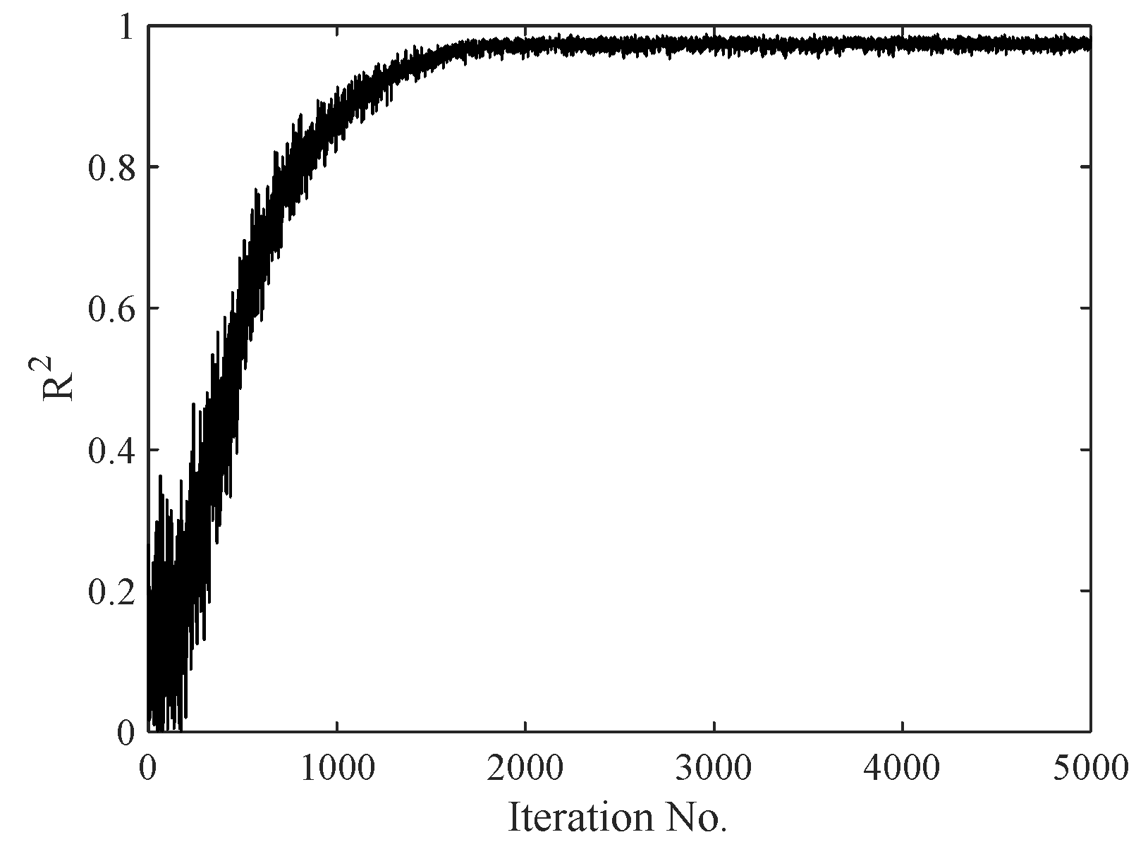
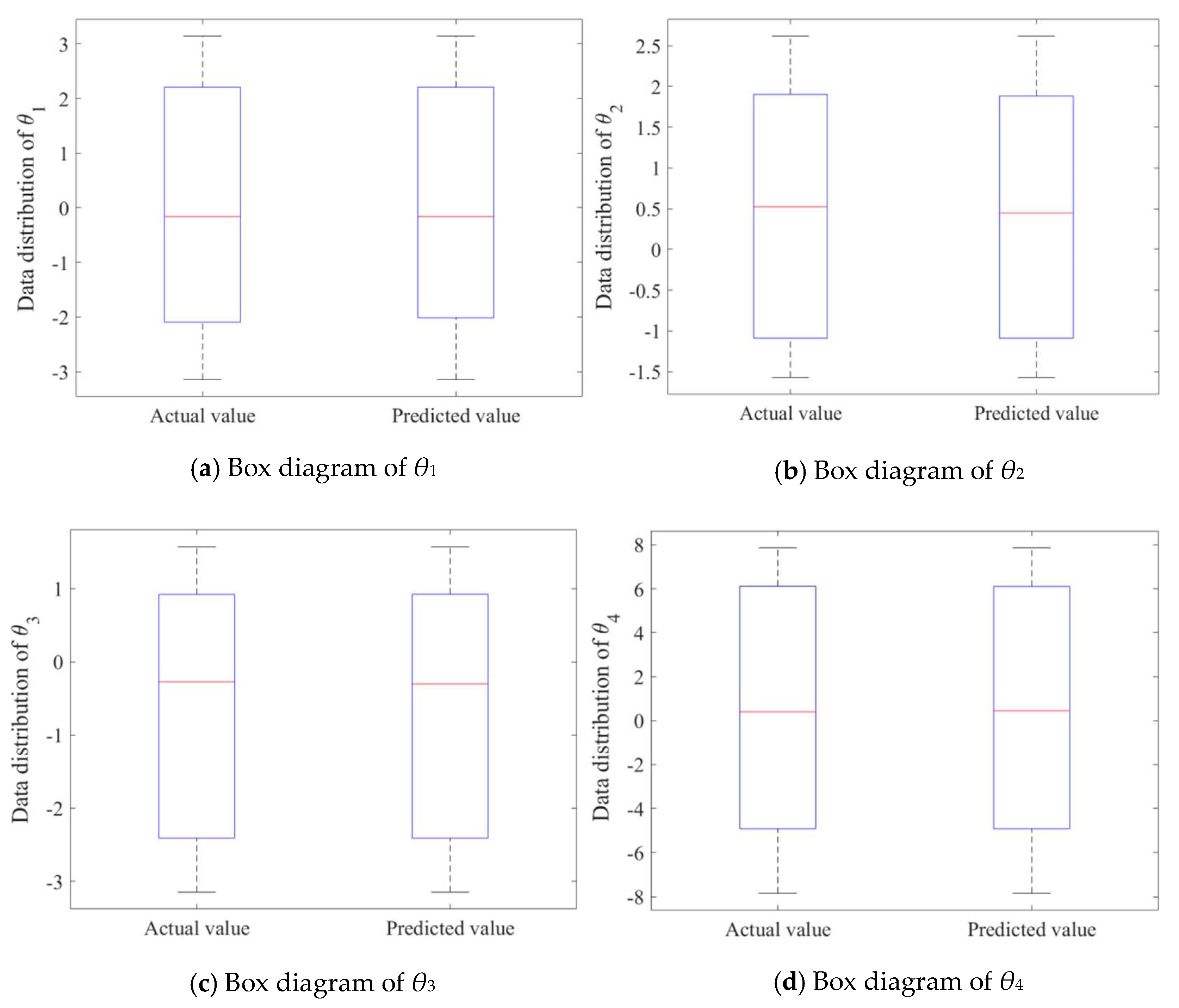
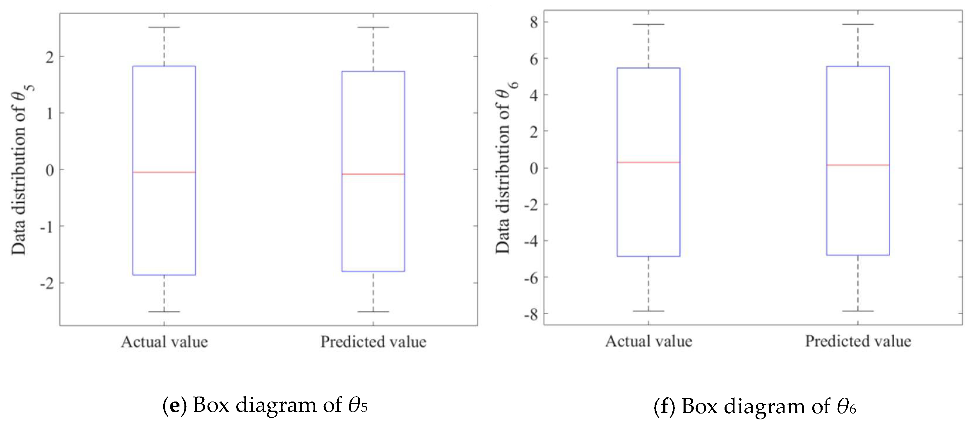
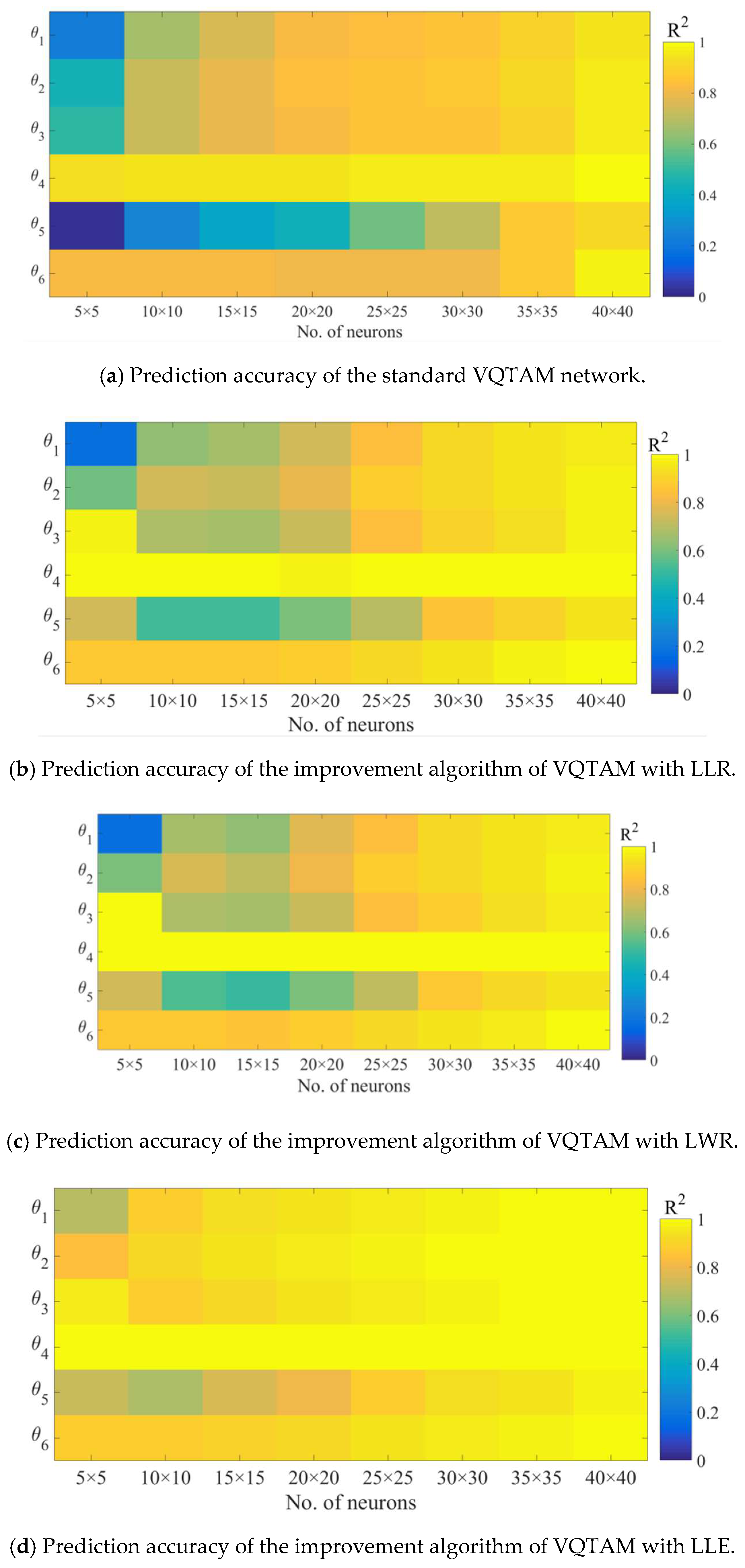
6.1. Standard VQTAM Network Test Results

According to the parameters of the robot shown in Table 1, the joint rotation angles for the sample set are generated as shown in Equations (38)–(43) [26,28]. The generated data can effectively cover the whole workspace of the manipulator.

$${\theta }_1(t)=\pi (1-e^{-\pi t})\cos 1.88\pi t$$

(38)

$${\theta }_2(t)=\frac{3}{2}\pi (1-e^{-\pi t})\sin 1.88\pi t+\pi /6$$

(39)

$${\theta }_3(t)=\frac{3}{4}\pi \cos t-\pi /4$$

(40)

$${\theta }_4(t)=\frac{5}{2}\pi \sin t$$

(41)

$${\theta }_5(t)=\frac{4}{5}\pi (1-e^{-\pi t})\sin 0.86\pi t$$

(42)

$${\theta }_6(t)=\frac{5}{2}\pi (1-e^{-\pi t})\sin 0.74\pi t$$

(43)

Taking time t ∈ [0,1000] and step t = 0.1, 10,001 joint angles Q(t) = [θ₁,θ₂,θ₃,θ₄,θ₅,θ₆] are calculated as the output of the sample set. The poses p(t) = [x,y,z;u,v,w] of the manipulator are calculated using the exponential coordinates of the motion screw, which are used as the input of the sample set. The VQTAM network is trained with the sample set Xⁱⁿ and X^out. In each epoch, 1000 pieces of data are selected randomly from the sample set, 80% of which are used as the training set and 20% as the test set. Meanwhile, to test the robustness of the algorithm, random errors are added to the test set data according to N(0,1) distribution.

The hyperparameter setting of the VQTAM network training is shown in

Table 3. Hyperparameter setting of VQTAM.

nq	np	epoch	α0	αM	σ0	σM
3	3	5000	0.8	0.001	15	0.001

. A VQTAM network with dimensions 60 × 60 (M_x × M_y) is trained based on the setting of hyperparameters, and the training effect is tested by the test set.

Root Mean Squared Error (RMSE), R-squared (R²), and Relative Maximum Absolute Error (RMAE) are used to evaluate the prediction accuracy of VQTAM for inverse kinematics, as shown in

Table 4. Root Mean Squared Error (RMSE), R-squared (R2), and Relative Maximum Absolute Error (RMAE) of the standard VQTAM network.

	θ1	θ2	θ3	θ4	θ5	θ6
RMSE	0.1871	0.1663	0.0895	0.2189	0.2459	0.5708
R2	0.9931	0.9808	0.9972	0.9984	0.9808	0.9894
RMAE	0.3914	0.6660	0.4840	0.1734	0.9828	0.5477

.

The value of R² ranges from 0 to 1. The closer it is to 1, the better the effect of regression fitting is, which means that the learning VQTAM network has higher accuracy as an approximate model. Generally, R² > 0.95 can be applied in engineering. For VQTAM networks with dimensions 60 × 60, the R² values after learning are all above 0.98. This shows that this network has value for engineering applications. RMSE and RMAE reflect the prediction error of the VQTAM network, and their small values also indicate the prediction accuracy of the network. The convergence result in the neural network training process is shown in Figure 6.

It can be seen from Figure 6 that the mean square R² of the VQTAM neural network tested by the test set in the training process gradually increases and converges near 1. This proves the effectiveness of the VQTAM neural network training algorithm.

The consistency between the actual data and the estimated data can be displayed more intuitively through box diagrams, as shown in Figure 7. It can be seen that the box diagrams of actual values and predicted values are very similar, which verifies the excellent prediction effect of the VQTAM network with dimensions 60 × 60.

6.2. VQTAM Local Linear Improvement Algorithms

The output of the inverse kinematics problem is estimated using the VQTAM local linear improvement algorithms. The priority K-means tree search algorithm is used to search the neighbor data of the input. The influence of parameter k on the prediction accuracy is analyzed, taking a VQTAM network with dimensions 35 × 35 as an example, as shown in Figure 8.

As can be seen from Figure 8, with the increase in k, R² increases continuously and approaches 1, which shows an increase in prediction accuracy. When k = 6, the R² for all variables is close to 1.

As can be seen from Figure 9, when k = 5, the R² for all variables is more than 0.95. When k = 6, R² is close to 1. Comparing Figure 8 and Figure 9, the overall prediction accuracy of the LWR algorithm is higher than that of the LLR algorithm.

As can be seen from Figure 8, when k = 5, the R² for all variables is greater than 0.99. Comparing Figure 8, Figure 9 and Figure 10, the overall prediction accuracy of the improvement algorithm of VQTAM with LLE is the highest.

In conclusion, when the number of neurons is small, the prediction accuracy of the network can be improved by combining local linear algorithms.

6.3. Overall Examples and Test Results

According to the VQTAM network hyperparameters shown in Table 3, the prediction accuracy of the four algorithms under different network dimensions (5 × 5, 10 × 10, 15 × 15, 20 × 20, 25 × 25, 30 × 30, 35 × 35, 40 × 40) is investigated, as shown in Figure 9. The number of the nearest nodes of the local linear algorithm is set to k = 6.

As can be seen from Figure 11, with the increase in the number of neurons, the prediction accuracy of the four algorithms significantly increases. The overall prediction accuracy of the improvement algorithm of VQTAM with LLE is the highest. The local linearization of VQTAM achieved remarkable results. Using the improved VQTAM algorithm, the estimation accuracy level of a network with dimensions of 35 × 35 is close to that of the standard VQTAM with dimensions of 60 × 60. Taking the improvement algorithm of VQTAM with LLE as an example, the output of the inverse kinematics, i.e., the rotation angles of six joints, is estimated, as shown in Figure 12. The estimated rotation angles of joints are compared with actual angles. It is shown that the VQTAM neural network can effectively estimate the output.

Substituting the joint rotation angle into the forward kinematics equation for calculation, the error of VQTAM can be obtained by comparing the result with the actual pose of the robot. The maximum error in the tool space is 3.9686 × 10⁻⁴ mm, and the average error is 4.6857 × 10⁻⁵ mm. This precision has met the control requirements of general robots in industrial applications.

The multilayer perceptron (MLP) can also provide the estimated results for the inverse kinematics. Thus, an MLP NARX network is trained for the comparison of prediction accuracy with VQTAM and its improvement algorithms. The MLP network has a hidden layer, and the number of hidden neurons is 3600. The sample set p(t), Q(t) for training MLP is the same as that for VQTAM. The Levenberg–Marquardt algorithm is chosen as the training algorithm. The comparison of prediction accuracy is shown in

Table 5. Comparison of prediction accuracy.

	MLP	VQTAM (60 × 60)	VQTAM (50 × 50)
RMSE	1.5935	0.2901	0.7823
	VQTAM with LLR (50 × 50)	VQTAM with LWR (50 × 50)	VQTAM with LLE (50 × 50)
RMSE	0.5163	0.6792	0.3018

.

The prediction accuracy of the standard VQTAM network is significantly higher than that of the MLP neuron network. Meanwhile, the prediction accuracy of the improvement algorithm of VQTAM also has better performance. The VQTAM is less sensitive to weight initialization than the MLP. Training multiple times will generate different results due to different initial conditions. The variation in the range of results of VQTAM is smaller. Compared with the results of a one-dimensional VQTAM in a previous study [27], the increase in dimensions improves the performance of the neural network.

7. Conclusions

The kinematics of the robotic manipulator is studied, and the forward kinematics solution method in the form of the exponential product of the screw is derived. Given the input angle of each joint of the robot, this method can be used to calculate the pose of the manipulator conveniently and quickly. It can also be used as the computational basis of a VQTAM network to establish sample sets.

A fast inverse kinematics mapping method for a robotic manipulator is proposed by using VQTAM for identification of nonlinear dynamic systems. The VQTAM algorithm is constructed to train and test the network. Based on the priority K-means tree search algorithm, the training, testing, and estimating processes of the VQTAM network are improved to enhance the search efficiency of nearest neighbors.

According to local neuron activation, the VQTAM network is improved based on local linearization. To further optimize the prediction accuracy of the network and reduce the dimensions of the network in application, VQTAM local linear improvement algorithms are proposed.

In this study, a sample data set for VQTAM training is constructed and the VQTAM algorithm and its improved algorithms are tested. The test results show that the increase in network dimensions can improve the prediction accuracy of VQTAM, but the computational efficiency is affected. By using VQTAM local linearization improvement algorithms, the estimation accuracy can be optimized for a low-dimensional network. When the search range is k = 6, the above algorithm can show good prediction accuracy, and the prediction effect of the LLE algorithm is the best among the three algorithms.

References

1. Mustafa, A.; Tyagi, C.; Verma, N.K. Inverse Kinematics Evaluation for Robotic Manipulator using Support Vector Regression and Kohonen Self Organizing Map. In Proceedings of the International Conference on Industrial and Information Systems, Roorkee, India, 3–4 December 2016; pp. 375–380. [Google Scholar]
2. Amouri, A.; Mahfoudi, C.; Zaatri, A.; Lakhal, O.; Merzouki, R. A Meta-heuristic Approach to Solve Inverse Kinematics of Continuum Manipulators. Available online: https://journals.sagepub.com/doi/abs/10.1177/0959651817700779 (accessed on 24 February 2020).
3. Jiang, L.; Huo, X.; Liu, Y.; Liu, H. An Analytical Inverse Kinematic Solution with the Reverse Coordinates for 6-DOF Manipulators. In Proceedings of the 2013 IEEE International Conference on Mechatronics and Automation, Takamatsu, Japan, 4–7 August 2013; pp. 1552–1558. [Google Scholar]
4. Sariyildiz, E.; Temeltas, H. Solution of Inverse Kinematic Problem for Serial Robot Using Quaternions. In Proceedings of the 2009 IEEE International Conference on Mechatronics and Automation, Singapore, 14–17 July 2009; pp. 26–31. [Google Scholar]
5. Sariyildiz, E.; Temeltas, H. A Comparison Study of Three Screw Theory Based Kinematic Solution Methods for the Industrial Robot Manipulators. In Proceedings of the 2011 IEEEInternational Conference on Mechatronics and Automation, Beijing, China, 7–10 August 2011; pp. 52–57. [Google Scholar]
6. Zhang, L.; Zuo, J.; Zhang, X.; Yao, X. A New Approach to Inverse Kinematic Solution for a Partially Decoupled Robot. In Proceedings of the 2015 International Conference on Control, Automation and Robotics, Singapore, 20–22 May 2015; pp. 55–59. [Google Scholar]
7. Sun, J.-D.; Cao, G.-Z.; Li, W.-B.; Liang, Y.-X.; Huang, S.-D. Analytical Inverse Kinematic Solution Using the D-H Method for a 6-DOF Robot. In Proceedings of the 2017 14th International Conference on Ubiquitous Robots and Ambient Intelligence, Jeju, South Korea, 28 June–1 July 2017; pp. 714–716. [Google Scholar]
8. Xin, S.Z.; Feng, L.Y.; Bing, H.L.; Li, Y.T. A Simple Method for Inverse Kinematic Analysis of the General 6R Serial Robot. In Proceedings of the ASME 2006 International Design Engineering Technical Conferences & Computers and Information in Engineering Conference, Philadelphia, PA, USA, 10–13 September 2006; pp. 1–8. [Google Scholar]
9. Joseph, C.; Musto, A. Two-Level Strategy for Optimizing the Reliability of Redundant Inverse Kinematic Solutions. J. Intell. Robot. Syst. 2002, 33, 73–84. [Google Scholar]
10. Wang, Y.; Sun, L.; Yan, W.; Liu, J. An Analytic and Optimal Inverse Kinematic Solution for a 7-DOF Space Manipulator. Robot 2014, 36, 592–599. [Google Scholar]
11. Chiaverini, S.; Ecgeland, O. An efficient pseudo-inverse solution to the inverse kinematic problem for six-joint manipulators. Model. Identif. Control 1990, 11, 201–222. [Google Scholar] [CrossRef] [Green Version]
12. Wang, W.; Suga, Y. Hiroyasu Iwata and Shigeki Sugano, Solve Inverse Kinematics Through A New Quadratic Minimization Technique. In Proceedings of the 2012 IEEE/ASME International Conference on Advanced Intelligent Mechatronics, Kachsiung, Taiwan, 11–14 July 2012; pp. 313–360. [Google Scholar]
13. Hargis, B.E.; Demirjian, W.A.; Powelson, M.W.; Canfield, S.L. Investigation of Neural-Network-Based Inverse Kinematics for A 6-DOF Serial Manipulator with Non-Spherical Wrist. In Proceedings of the ASME 2018 International Design Engineering Technical Conferences and Computers and Information in Engineering Conference, Quebec City, QC, Canada, 26–29August 2018; pp. 1–14. [Google Scholar]
14. Lou, Y.F.; Brunn, P. A hybrid artificial neural network inverse kinematic solution for accurate robot path control. Proc. Inst. Mech. Eng. Part I J. Syst. Control Eng. 1999, 213, 23–32. [Google Scholar] [CrossRef]
15. Mahajan, A.; Singh, H.P.; Sukavanam, N. An unsupervised learning based neural network approach for a robotic manipulator. Int. J. Inf. Technol. 2017, 9, 1–6. [Google Scholar] [CrossRef]
16. Kenwright, B. Neural Network in Combination with a Differential Evolutionary Training Algorithm for Addressing Ambiguous Articulated Inverse Kinematic Problems. In Proceedings of the 11th ACM SIGGRAPH Conference and Exhibition on Computer Graphics and Interactive Techniques in Asia, Tokyo, JAPAN, 4–7 December 2018. [Google Scholar]
17. Kinoshita, K. Estimation of Inverse Model by PSO and Simultaneous Perturbation Method. In Proceedings of the 2015 Seventh International Conference of Soft Computing and Pattern Recognition, Fukuoka, Japan, 13–15 November 2015; pp. 48–53. [Google Scholar]
18. Rui, T.; Zhu, J.-W.; Zhou, Y.; Ma, G.-Y.; Yao, T. Inverse Kinematics Analysis of Multi-DOFs Serial Manipulators Based on PSO. J. Syst. Simul. 2009, 21, 2930–2932. [Google Scholar]
19. Shihabudheen, K.V.; Pillai, G.N. Evolutionary Fuzzy Extreme Learning Machine for Inverse Kinematic Modeling of Robotic Arms. In Proceedings of the 2015 39th National Systems Conference, Noida, India, 14–16 December 2015. [Google Scholar]
20. Oyama, E.; Maeda, T.; Gan, J.Q.; Rosales, E.M.; MacDorman, K.F.; Tachi, S.; Agah, A. Inverse kinematics learning for robotic arms with fewer degrees of freedom by modular neural network systems. In Proceedings of the 2005 IEEE/RSJ International Conference on Intelligent Robots and Systems, Edmonton, AB, Canada, 2–6 August 2005; pp. 1791–1798. [Google Scholar]
21. Wu, X.; Xie, Z. Forward kinematics analysis of a novel 3-DOF parallel manipulator. Sci. Iran. 2019, 26, 346–357. [Google Scholar] [CrossRef] [Green Version]
22. Pham, D.T.; Castellani, M.; Fahmy, A.A. Learning the inverse kinematics of a robot manipulator using the Bees algorithm. In Proceedings of the 2008 6th IEEE International Conference on Industrial Informatics, Daejeon, South Korea, 13–16 July 2008; pp. 493–498. [Google Scholar]
23. Giorelli, M.; Renda, F.; Calisti, M.; Arienti, A.; Ferri, G.; Laschi, C. Learning the inverse kinetics of an octopus-like manipulator in three-dimensional space. Bioinspir. Biomim. 2015, 10, 035006. [Google Scholar] [CrossRef] [PubMed] [Green Version]
24. Karkalos, N.E.; Markopoulos, A.P.; Dossis, M.F. Optimal Model Parameters of Inverse Kinematics Solution of a 3R Robotic Manipulator Using Ann Models. Int. J. Manuf. Mater. Mech. Eng. 2017, 7, 20–40. [Google Scholar] [CrossRef]
25. Rong, P.-X.; Yang, Y.-J.; Hu, L.-G.; Ma, G.-F. Inverse kinematic in SCARA manipulator based on RBF networks. Electr. Mach. 2007, 11, 303–305. [Google Scholar]
26. Kumar, P.R.; Bandyopadhyay, B. The Forward Kinematic Modeling of a Stewart Platform using NLARX Model with Wavelet Network. In Proceedings of the IEEE International Conference on Industrial Informatics, Bochum, Germany, 29–31 July 2013; pp. 343–348. [Google Scholar]
27. Barreto, G.D.; Araujo, A.F.R. Temporal associative memory and function approximation with the self-organizing map. In Proceedings of the Neural Networks For Signal Processing Xii, Martigny, Switzerland, 6 September 2002; pp. 109–118. [Google Scholar]
28. Limtrakul, S.; Arnonkijpanich, B. Supervised learning based on the self-organizing maps for forward kinematic modeling of Stewart platform. Neural Comput. Appl. 2019, 31, 619–635. [Google Scholar] [CrossRef]
29. Heskes, T. Self-organizing maps, vector quantization, and mixture modeling. IEEE Trans. Neural Netw. 2001, 12, 1299–1305. [Google Scholar] [CrossRef] [PubMed]
30. Zhu, S.; Chen, Q.; Wang, X.; Liu, S. Dynamic modeling using screw theory and nonlinear sliding mode control of series robot. Int. J. Robot. Autom. 2016, 31, 63–75. [Google Scholar]
31. Chen, Q.; Zhu, S.; Zhang, X. An Improved Inverse Kinematic Algorithm for 6 DOF Serial Robot Using Screw Theory. Int. J. Adv. Robot. Syst. 2015, 12, 140. [Google Scholar] [CrossRef]
32. Muja, M.; Lowe, D.G. Scalable Nearest Neighbor Algorithms for High Dimensional Data. IEEE Trans. Pattern Anal. Mach. Intell. 2014, 36, 2227–2240. [Google Scholar] [CrossRef] [PubMed]
Figure 1. Research content and structure.
Symmetry 12 00519 g001
Figure 2. Six-degree of freedom (6-DOF) robotic manipulator (RRRRRR type).
Symmetry 12 00519 g002
Figure 3. Poses corresponding to Table 2.
Symmetry 12 00519 g003
Figure 4. Vector-Quantified Temporal Associative Memory (VQTAM) spatial mapping.
Symmetry 12 00519 g004
Figure 5. Local linearization of the VQTAM network.
Symmetry 12 00519 g005
Figure 6. Convergence result.
Symmetry 12 00519 g006
Figure 7. Box diagrams of the VQTAM network prediction effect.
Symmetry 12 00519 g007aSymmetry 12 00519 g007b
Figure 8. The influence of k-nearest neighbor number in the improvement algorithm of VQTAM with Local Linear Regression (LLR).
Symmetry 12 00519 g008
Figure 9. The influence of k-nearest neighbor number in the improvement algorithm of VQTAM with Local Weighted Linear Regression (LWR).
Symmetry 12 00519 g009
Figure 10. The influence of k-nearest neighbor number in the improvement algorithm of VQTAM with Local Linear Embedding (LLE).
Symmetry 12 00519 g010
Figure 11. Prediction accuracy of 4 algorithms.
Symmetry 12 00519 g011
Figure 12. Inverse kinematics output estimation.
Symmetry 12 00519 g012