Convergence and Dynamics of a Higher-Order Method

 ,
,  ,
,  ,
,  and
and 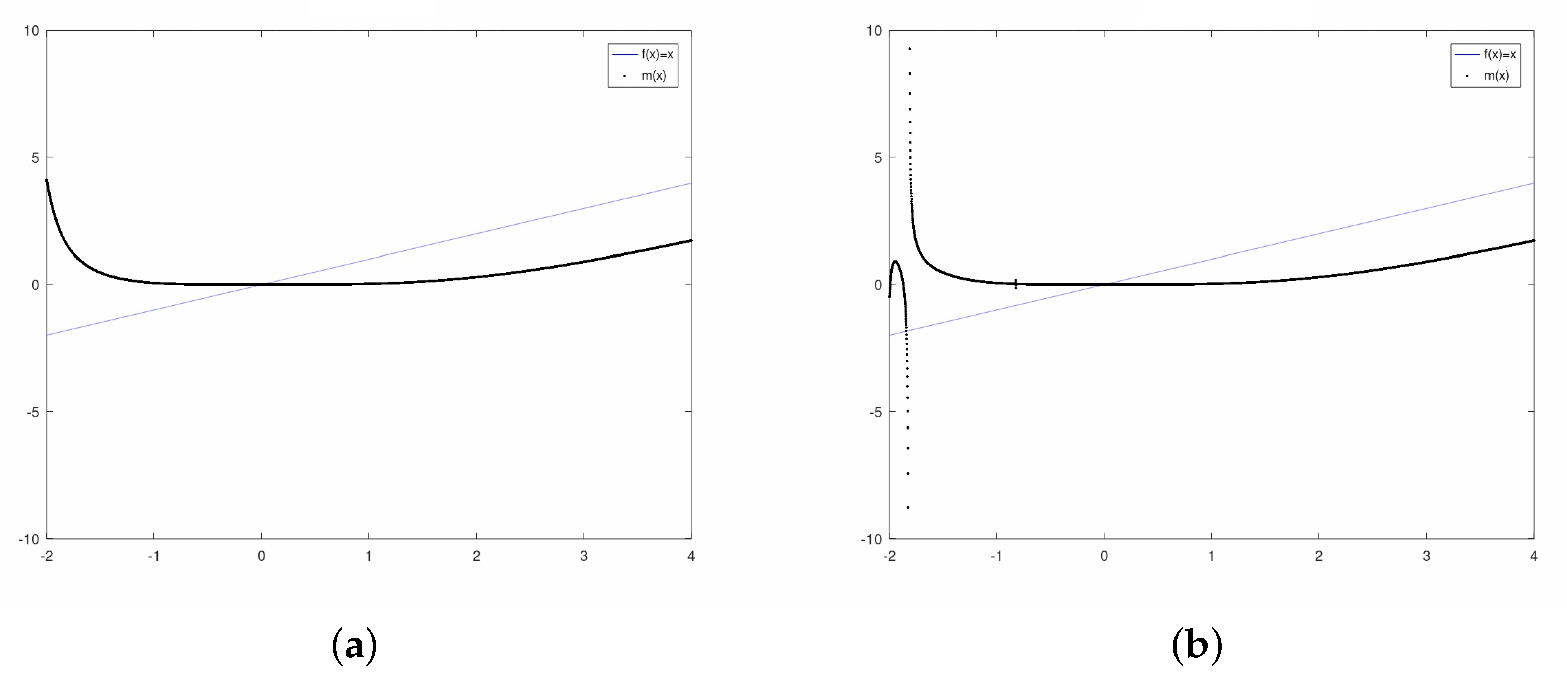
Abstract
1. Introduction
2. Local Convergence Analysis
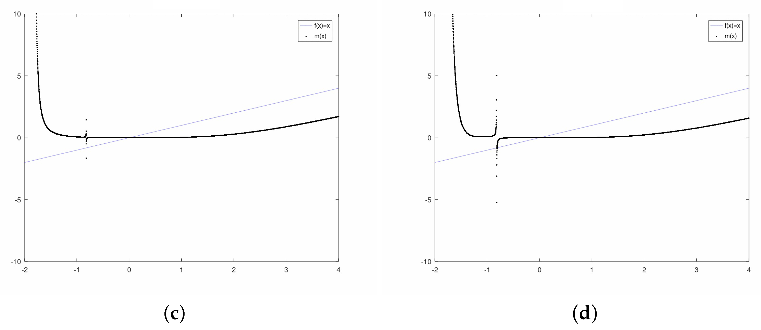
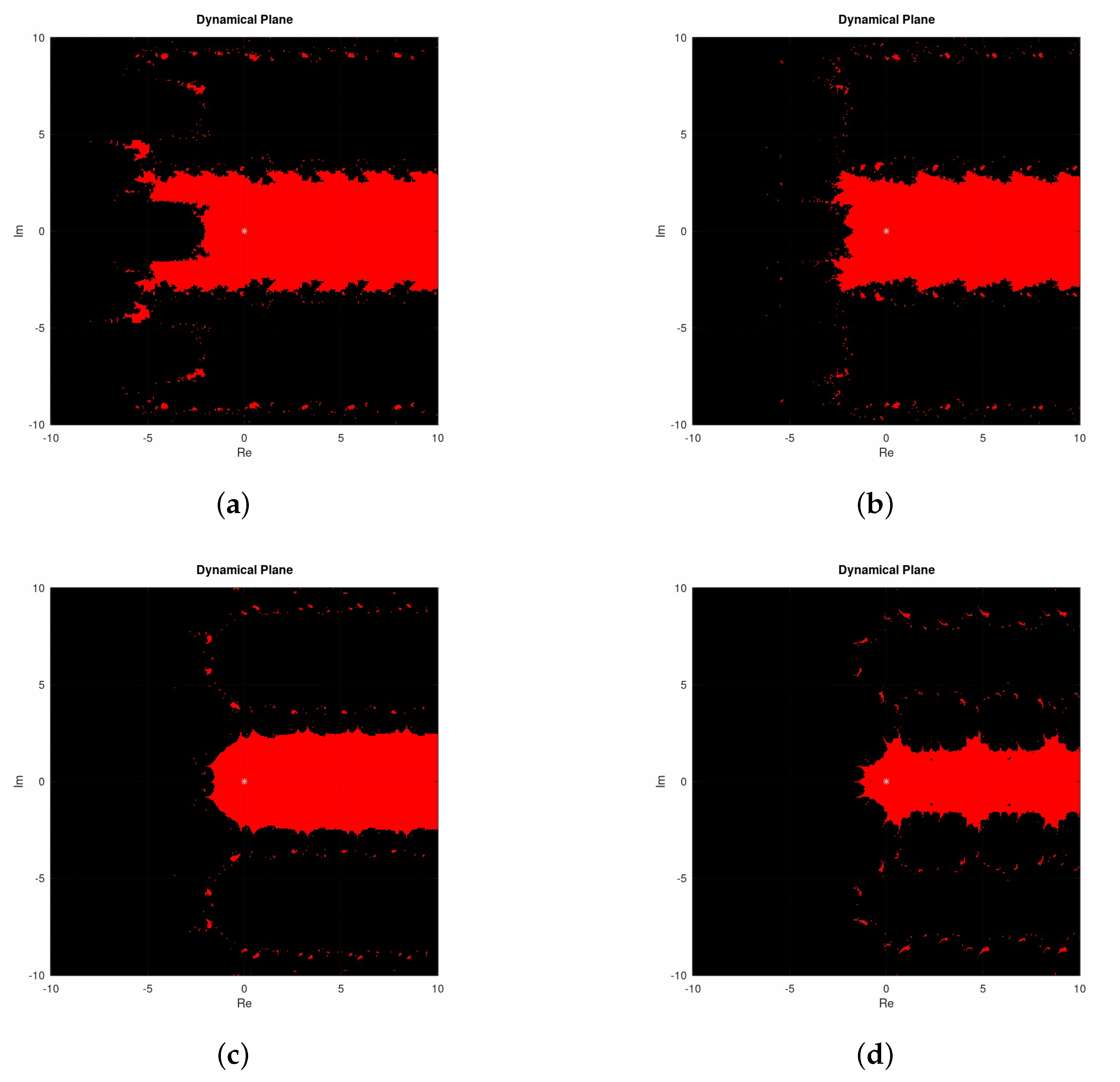
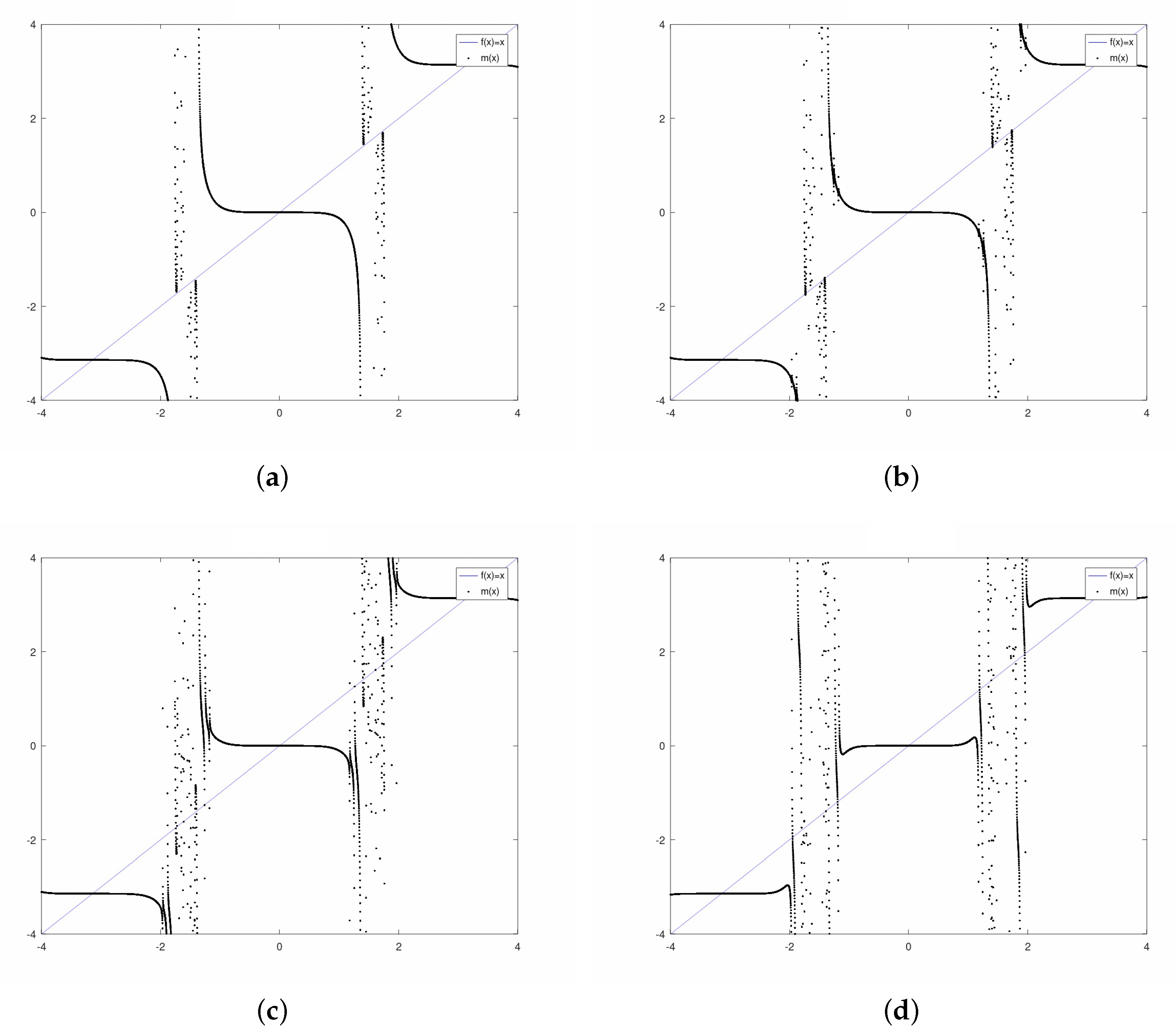
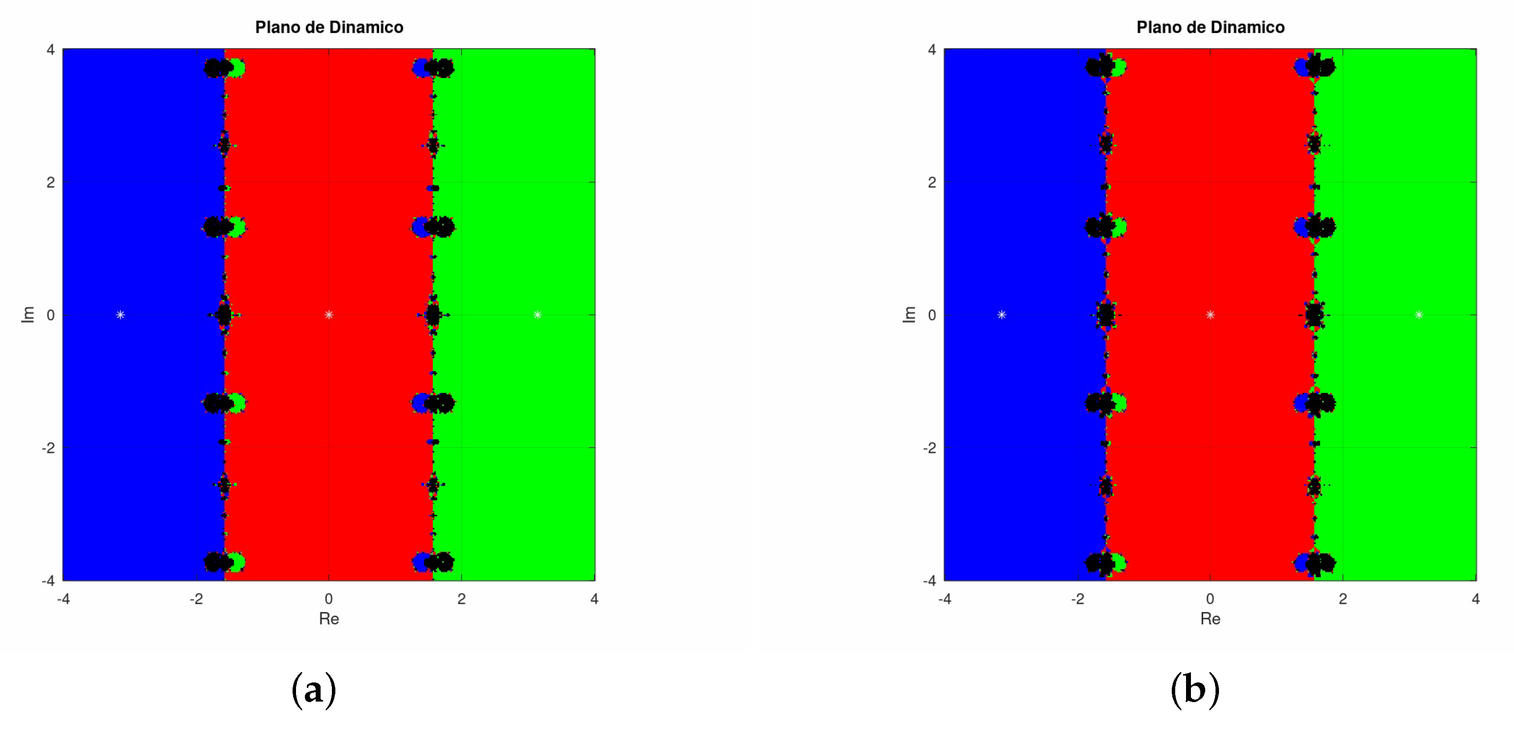
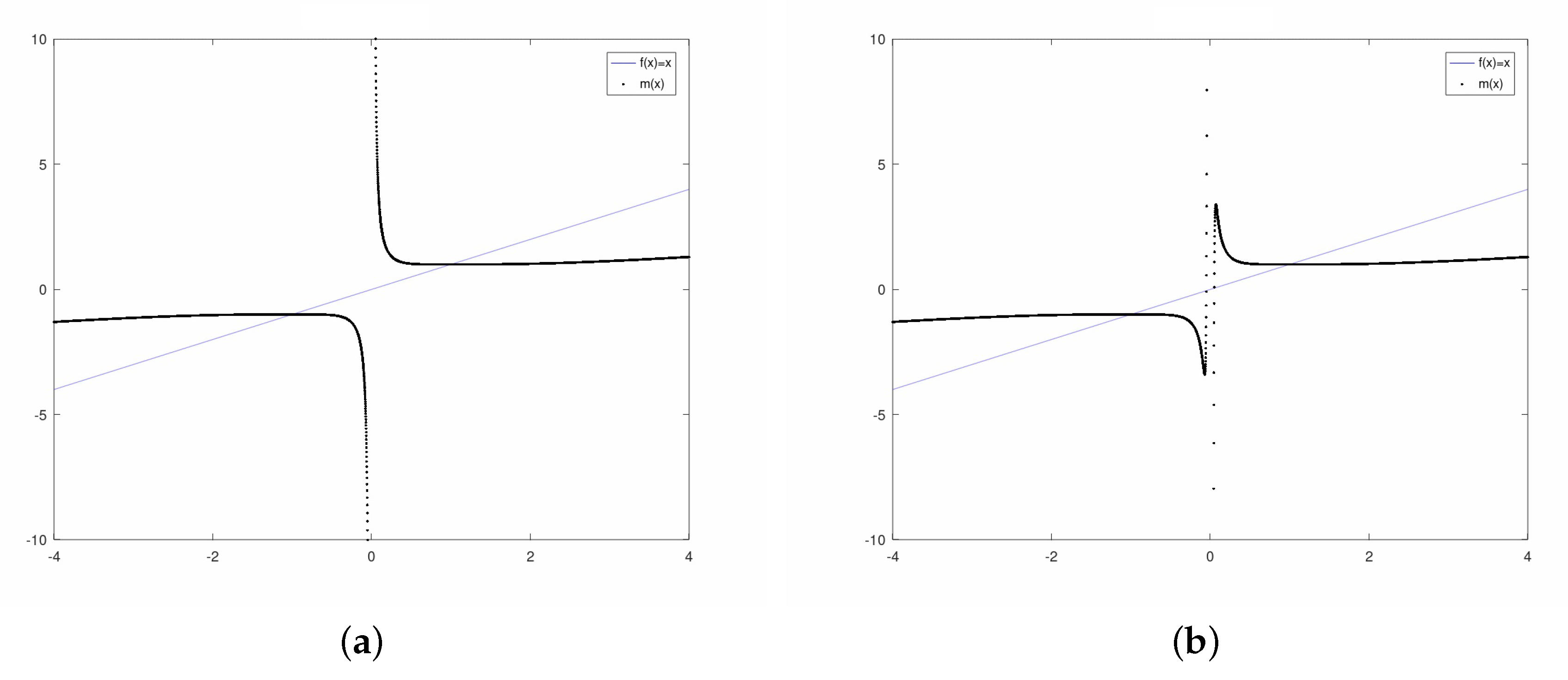
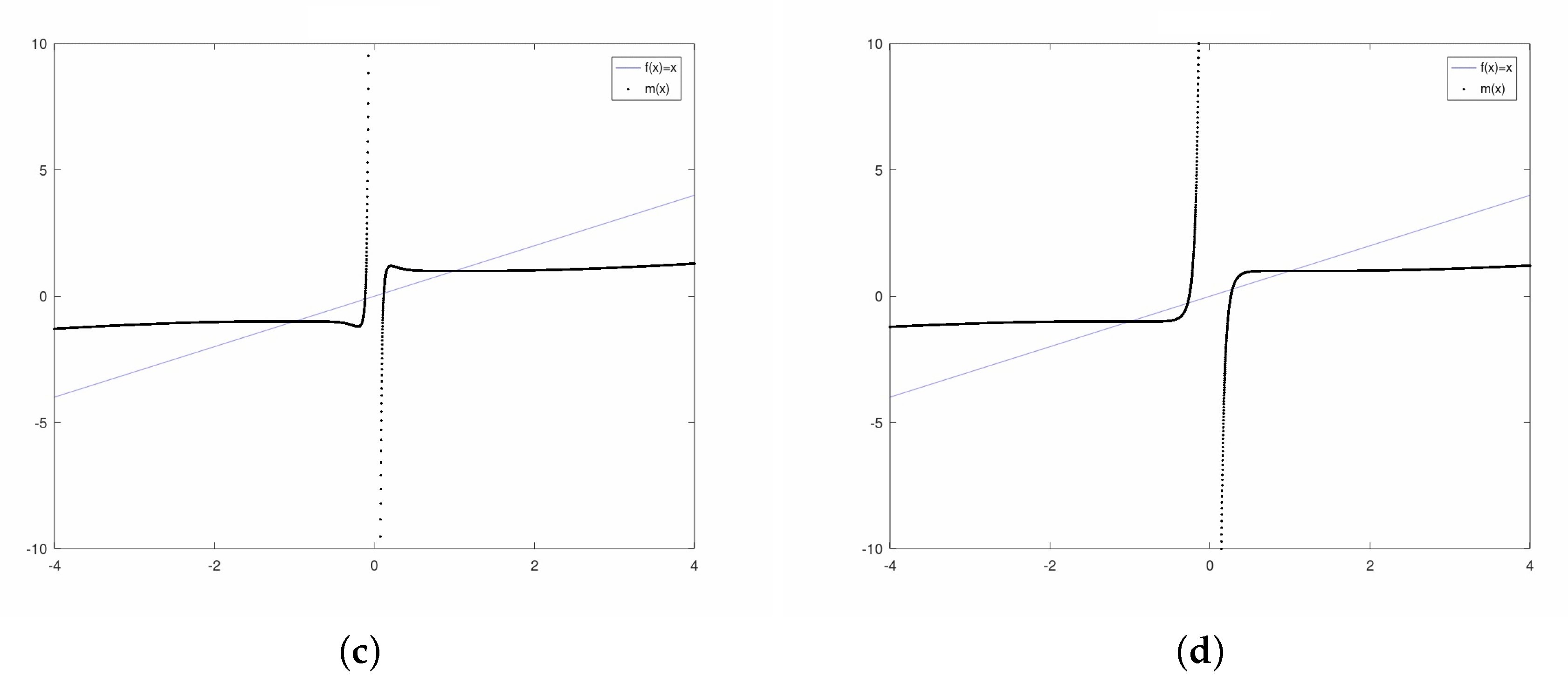
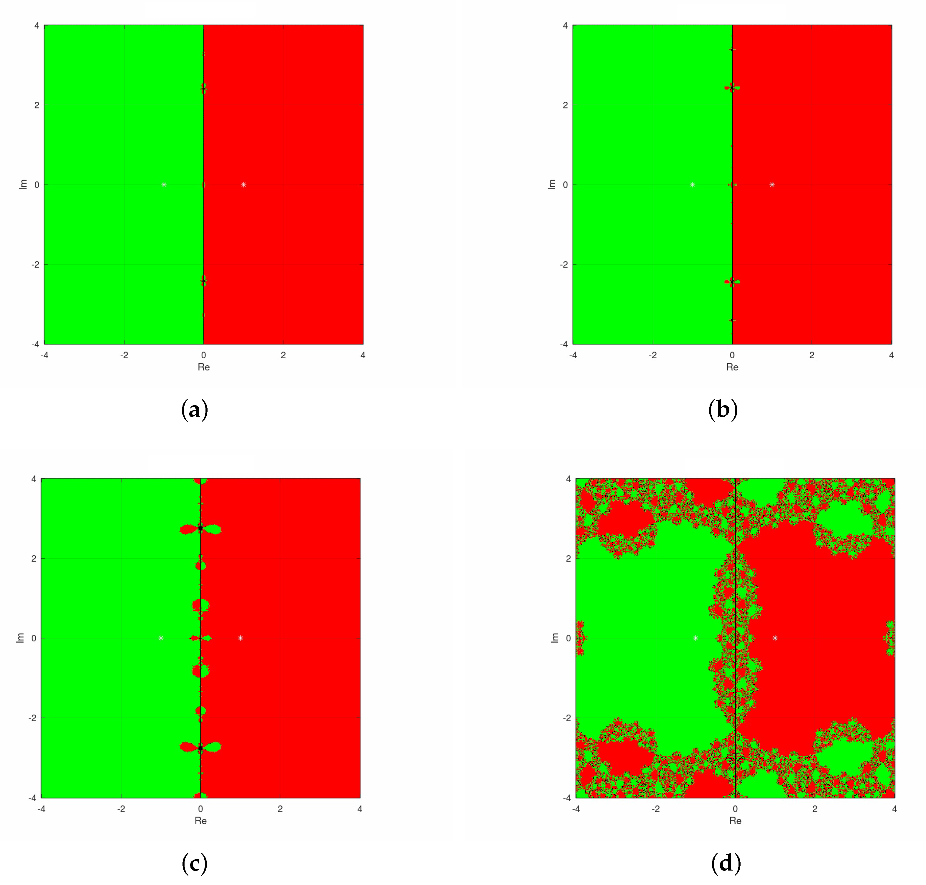
3. Dynamical Analysis
3.1. Exponential Family
3.2. Sinus Family
3.3. Polynomial Family
4. Conclusions
Author Contributions
Funding
Acknowledgments
Conflicts of Interest
References
- Petković, M.S.; Neta, B.; Petković, L.D.; Dźunić, J. Multipoint Methods for Solving Nonlinear Equations: A Survey; Elsevier: Amsterdam, The Netherlands, 2013. [Google Scholar]
- Hueso, J.L.; Martinez, E.; Teruel, C. Convergence, efficiency and dynamics of new fourth and sixth order families of iterative methods for nonlinear systems. J. Comput. Appl. Math. 2015, 275, 412–420. [Google Scholar] [CrossRef]
- Behl, R.; Kanwar, V.; Kim, Y.I. Higher-order families of multiple root finding methods suitable for non-convergent cases and their dynamics. Math. Model. Anal. 2019, 24, 422–444. [Google Scholar] [CrossRef]
- Amat, S.; Busquier, S.; Gutiérrez, J.M. Geometric constructions of iterative functions to solve nonlinear equations. J. Comput. Appl. Math. 2003, 157, 197–205. [Google Scholar] [CrossRef]
- Argyros, I.K. Computational Theory of Iterative Methods. Series: Studies in Computational Mathematics, 15; Chui, C.K., Wuytack, L., Eds.; Elsevier Publ. Co.: New York, NY, USA, 2007. [Google Scholar]
- Argyros, I.K.; Magreñán, Á.A. Iterative Methods and Their Dynamics with Applications: A Contemporary Study; CRC Press: Boca Raton, FL, USA; Taylor & Francis Group: Abingdon, UK, 2017. [Google Scholar]
- Argyros, I.K.; Magreñán, Á.A. A Contemporary Study of Iterative Methods: Convergence, Dynamics and Applications; Elsevier: Amsterdam, The Netherlands, 2017. [Google Scholar]
- Argyros, I.K.; Hilout, S. Computational Methods in Nonlinear Analysis. Efficient Algorithms, Fixed Point Theory and Applications; World Scientific: Singapore, 2013. [Google Scholar]
- Argyros, I.K.; Hilout, S. Numerical Methods in Nonlinear Analysis; World Scientific Publ. Comp.: Hackensack, NJ, USA, 2013. [Google Scholar]
- Kantorovich, L.V.; Akilov, G.P. Functional Analysis; Pergamon Press: Oxford, UK, 1982. [Google Scholar]
- Ortega, J.M.; Rheinboldt, W.C. Iterative Solution of Nonlinear Equations in Several Variables; Academic Press: New York, NY, USA, 1970. [Google Scholar]
- Rheinboldt, W.C. An adaptive continuation process for solving systems of nonlinear equations, Polish Academy of Science. Banach Ctr. Publ. 1978, 3, 129–142. [Google Scholar] [CrossRef]
- Sharma, J.R. Improved Chebyshev–Halley methods with sixth and eighth order of convergence. Appl. Math. Comput. 2015, 256, 119–124. [Google Scholar] [CrossRef]
- Sharma, R. Some fifth and sixth order iterative methods for solving nonlinear equations. Int. J. Eng. Res. Appl. 2014, 4, 268–273. [Google Scholar]
- Traub, J.F. Iterative Methods for the Solution of Equations; Prentice–Hall Series in Automatic Computation: Englewood Cliffs, NJ, USA, 1964. [Google Scholar]
- Madhu, K.; Jayaraman, J. Higher Order Methods for Nonlinear Equations and Their Basins of Attraction. Mathematics 2016, 4, 22. [Google Scholar] [CrossRef]
- Sanz-Serna, J.M.; Zhu, B. Word series high-order averaging of highly oscillatory differential equations with delay. Appl. Math. Nonlinear Sci. 2019, 4, 445–454. [Google Scholar] [CrossRef]
- Pandey, P.K. A new computational algorithm for the solution of second order initial value problems in ordinary differential equations. Appl. Math. Nonlinear Sci. 2018, 3, 167–174. [Google Scholar] [CrossRef]
- Magreñán, Á.A. Different anomalies in a Jarratt family of iterative root–finding methods. Appl. Math. Comput. 2014, 233, 29–38. [Google Scholar]
- Magreñán, Á.A. A new tool to study real dynamics: The convergence plane. Appl. Math. Comput. 2014, 248, 215–224. [Google Scholar] [CrossRef]
- Magreñán, Á.A.; Argyros, I.K. On the local convergence and the dynamics of Chebyshev-Halley methods with six and eight order of convergence. J. Comput. Appl. Math. 2016, 298, 236–251. [Google Scholar] [CrossRef]
- Lotfi, T.; Magreñán, Á.A.; Mahdiani, K.; Rainer, J.J. A variant of Steffensen-King’s type family with accelerated sixth-order convergence and high efficiency index: Dynamic study and approach. Appl. Math. Comput. 2015, 252, 347–353. [Google Scholar] [CrossRef]


© 2020 by the authors. Licensee MDPI, Basel, Switzerland. This article is an open access article distributed under the terms and conditions of the Creative Commons Attribution (CC BY) license (http://creativecommons.org/licenses/by/4.0/).
Share and Cite
Moysi, A.; Argyros, I.K.; Regmi, S.; González, D.; Magreñán, Á.A.; Sicilia, J.A. Convergence and Dynamics of a Higher-Order Method. Symmetry 2020, 12, 420. https://doi.org/10.3390/sym12030420
Moysi A, Argyros IK, Regmi S, González D, Magreñán ÁA, Sicilia JA. Convergence and Dynamics of a Higher-Order Method. Symmetry. 2020; 12(3):420. https://doi.org/10.3390/sym12030420
Chicago/Turabian StyleMoysi, Alejandro, Ioannis K. Argyros, Samundra Regmi, Daniel González, Á. Alberto Magreñán, and Juan Antonio Sicilia. 2020. "Convergence and Dynamics of a Higher-Order Method" Symmetry 12, no. 3: 420. https://doi.org/10.3390/sym12030420
APA StyleMoysi, A., Argyros, I. K., Regmi, S., González, D., Magreñán, Á. A., & Sicilia, J. A. (2020). Convergence and Dynamics of a Higher-Order Method. Symmetry, 12(3), 420. https://doi.org/10.3390/sym12030420