Free Vibration of AFG Circular Arch with Symmetric and Anti-symmetric Boundary Conditions at Mid-Arc

Abstract

This paper studies the in-plane free vibration of axially functionally graded (AFG) circular arches with non-uniform cross-section. The geometric and material properties of circular arches with regular polygon cross-section vary symmetrically about the mid-arc along the axial direction in quadratic polynomial form. The governing differential equations of the motion are derived, and the symmetric and anti-symmetric boundary conditions of the arches are developed for applying initial and boundary value problems in the solution method. The computed results agree well with the results of the finite element software ADINA. The effects of geometrical and material parameters on the natural frequency and mode shape of AFG circular arches are investigated.

1. Introduction

Using certain structural conditions such as boundary conditions makes it easier to analyze complex structural systems. For symmetric structural analysis such as square plate, only a quarter section of the structural body from the entire analysis area can be considered if the symmetry conditions apply. This concept of analysis has been widely used in the finite element method. In this respect, this study considers a novel structural analyzing method using the symmetry conditions of the symmetric structures.

Arched member is one of the important units that are commonly used in engineering applications. The functionally graded materials (FGMs) have become widely used for engineering purposes because of their advantages over conventional materials [1]. The tapered members work distinctively from the prismatic member because the tapered cross-section yields effective stress distributions and a strong coupling between the stress resultants. Understanding the vibration behavior of structural systems is essential to the design, construction, and maintenance of structures [2]. Considering the research topics stated above, this paper focuses on the free vibration of tapered arch made of axially FGMs to apply the symmetric conditions of the structures.

The following studies and their citations include mathematical models and historical reviews related to topics of this paper. For functionally graded beams/columns, much study has been conducted: Li [3] studied dynamic behaviors of the prismatic beam, including effects of the rotatory inertia and shear deformation; Kukla and Rychlewska [4] investigated free vibrations of clamped beams made of two different FGMs; Elishakoff et al. [5] studied the free vibration of columns with Duncan’s mode shape by considering a fifth-order polynomial based on the Rayleigh-Ritz method; Rezaiee and Masoodi [6] investigated exact natural frequencies of the tapered beam-columns; Huang and Li [7] investigated a novel approach for analyzing the free vibration of tapered beams; Shahba and Rajasekaran [8] conducted the stability analysis of tapered beams where the governing equations for free vibration were solved using the differential transform element method (DTEM); Rajasekaran [9] studied the natural frequencies of Timoshenko beams using DTEM; and Akgoz and Civalek [10] studied free vibrations of the tapered rectangular functionally graded microbeam based on the modified couple stress theory. Chandran and Rajendran [11] and Ranganathan et al. [12] studied the buckling of columns. On the other hand, Carrera et al. [13] investigated the Layer-Wise (LW) models for the electro-mechanical analysis of shell-structures with applied symmetry boundary-conditions.

In particular, for functionally graded arches directly related to this study, very little research was carried out. Malekzadeh et al. [14,15] studied free vibrations of the arch with temperature-dependent properties which is more applicable to laterally functionally graded arch. For AFG arch, Rajasekaran [16] investigated the free vibration of the parabolic arch using DTEM; Noori et al. [17] studied forced vibrations of the parabolic arch using the complementary functions method combined with the Laplace transform; and Lee and Lee [18] studied the free vibration of uniform circular AFG arch. Most of previous works, however, have focused on the arches of conventional cross-section (e.g., circle and rectangle) with homogenous properties in the axial direction. In contrast, the study of arches with regular polygon cross-section and material inhomogeneity has not reported in literature.

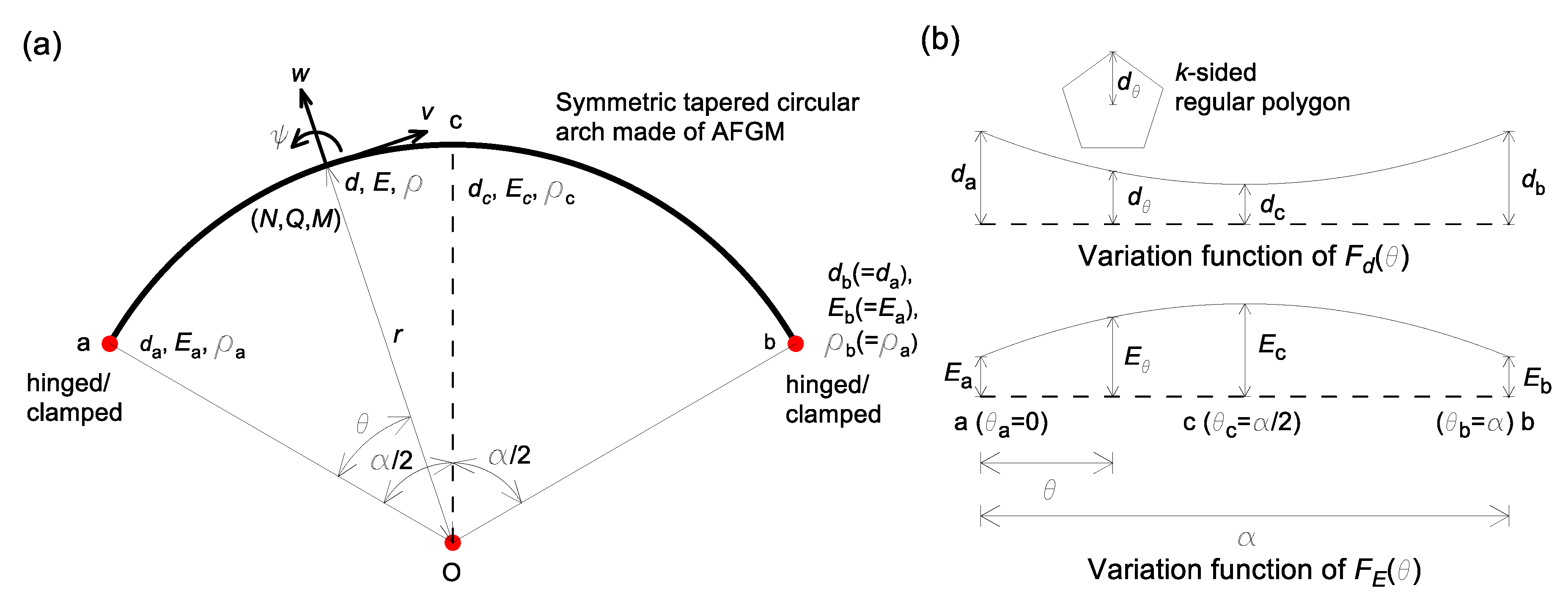
This paper presents differential equations that govern the free vibration of a tapered AFG circular arch with regular polygon cross-section including the rotatory inertia couple. To calculate natural frequencies and mode shapes of the arch, the governing equations are solved numerically using the boundary conditions, i.e., symmetric and anti-symmetric boundary conditions [19], at the mid-arc of the arch as the initial and boundary value problems. For verification purpose, the predicted natural frequencies are compared with those of the finite element software ADINA. Parametric studies on natural frequencies of the arch are extensively discussed and the mode shapes are reported.

The following assumptions were made to formulate the mathematical models: AFG circular arch is linear elastic, the shear deformation effect is negligible, the deformation is small, and the free vibration is based on the harmonic motion. In addition, the variable functions of the taper and the mechanical property of the arch are assumed to be a univariate quadratic polynomial.

2. Problem Formulation

2.1. Configuration of Symmetric Circular Arch

Figure 1a shows the configuration of a symmetric circular arch with radius $r$ and subtended angle $\alpha$. The arch axis is defined as a planar structure in polar coordinates $\left(r,\theta \right)$. Both ends (i.e., the left end $\mathrm{a}$ $\left(\theta = 0\right)$ and the right end $\mathrm{b}$ $(\theta = \alpha$)) are supported by hinged or clamped ends. Since the shape of the arch is symmetrical, both hinged ($\mathrm{H}-\mathrm{H}$) and both clamped ($\mathrm{C}-\mathrm{C}$) end conditions are considered in this study. Afterwards, the end condition of the arch is indicated by $‘\mathrm{H}-\mathrm{H}’$ and $‘\mathrm{C}-\mathrm{C}’$, respectively, as described in parentheses. Figure 1b depicts the variable function of the taper and the mechanical property of arch. The arch cross-section is tapered symmetrically about the mid-arc $\mathrm{c}(\theta = \alpha /2).$ The cross-sectional shape is $k\left(\ge 3\right)$-sided regular polygon with a radial depth $d$ defined as a length measured from the centroid to the vertex. Here, $k$ is the integer side number of the regular polygon. At both ends, $d$ is represented by $d_a$ and $d_b\left(= d_a\right)$, respectively, and at the mid-arc by $d_c$. Depth $d$ varies symmetrically as a function of $\theta$. As a result, changes of the area $A$and the moment of inertia of plane area $I$ are symmetric about the mid-arc. The arch is made of AFGM. The mechanical properties of the Young’s modulus $E$and the mass density $\rho$ vary with the polar coordinate $\theta$ along the arch axis. At both ends, Young’s modulus and mass density are represented by $(E_a,{\rho }_a)$ and $(E_b,{\rho }_b)$, respectively, and at the mid-arc by $(E_c,{\rho }_c)$. It is noted that $E_b = E_a$ and ${\rho }_b = {\rho }_a$. Consequently, the changes in $E$and $\rho$ are symmetric about the mid-arc. Thus, as described above, all configuration of the arch is completely symmetric, including the arch curvilinear, the end condition, the variations of the taper and mechanical property along the axis direction.

When the AFG arch vibrates, the dynamic radial and tangential deflections (amplitudes) $w$ and $v$ and the dynamic rotation $\psi$ occur at $\left(r,\theta \right)$, and also dynamic stress resultants of the axial force $N$, the shear force $Q$, and the bending moment $M$ shown in Figure 1a occur at $\left(r,\theta \right)$.

The variable functions of $E$ and $\rho$ are now defined. The function of Young’s modulus $E$ of AFGM is arbitrary, such as linear [8,11,13], polynomial [3,5,6,7,12,18], exponential [4,7,16,17], and periodic [7,12] functions previously reported in the literature. In this study, the function $E$ is chosen as a quadratic polynomial based on a single variable $\theta$. It assumes that the function of $\rho$ is the same as that of $E$ [3,4,5,6,7,8,9,10,18]. To define the quadratic polynomials of $E$ and $\rho$, the modular ratio $m$ of $E_a$ to $E_c$ (equal to the density ratio of ${\rho }_a$ to ${\rho }_c$) is introduced as:

$$m =\frac{E_a}{E_c}\left( = \frac{{\rho }_a}{{\rho }_c}\right)$$

(1)

Using Equation (1), the $E$ and $\rho$ at $\left(r,\theta \right)$ are can be expressed in the quadratic polynomial form:

$$E =E_c{F}_E;\rho ={\rho }_c{F}_E$$

(2)

where $F_E = m_1\left({\theta }^2/{\alpha }^2-\theta /\alpha \right)+m$ and $m_1 = 4\left(m-1\right)$. See $F_E$ function $(m >1)$ in Figure 1b.

Now defined is the variable function $d$ of the tapered cross-section. The taper ratio $n$ is introduced as a ratio of $d_a$ to $d_c$, or

$$n =\frac{d_a}{d_c}$$

(3)

The variable function $d$ can be expressed as an arbitrary function of $\theta$. In this study, a quadratic polynomial function is selected as:

$$d =d_c{F}_d$$

(4)

where $F_d = n_1\left({\theta }^2/{\alpha }^2-\theta /\alpha \right)+n$, $n_1 = 4\left(n-1\right)$ and $d$ with $0\le n <1$ is concave, $d$ with $n = 1$ is uniform, and $d$ with $n > 1$ is convex. See $F_d$ function with $0\le n <1$ in Figure 1b.

Using the function $d$ in Equation (4), the variable functions $\left(A,I\right)$ for $k$-sided regular polygonal cross-section at $\left(r,\theta \right)$ are obtained as:

$$A =c_1{d}^2 = c_1{d}_c^2{F}_d^2;I =c_2{d}^4 = c_2{d}_c^4{F}_d^4$$

(5)

where constants $c_1$ and $c_2$ are given as [20]:

$$c_1 = k\sin \left(\frac{\pi }{k}\right)\cos \left(\frac{\pi }{k}\right);c_2 = \frac{k}{12}\sin \left(\frac{\pi }{k}\right){\cos }^3\left(\frac{\pi }{k}\right)\left[3+{\tan }^2\left(\frac{\pi }{k}\right)\right]$$

(6)

2.2. Governing Differential Equations

When the arch vibrates, the stresses resultants in axial force $N$, shear force $Q$ and bending moment $M$ due to the dynamic deformations $(w$, $v$, $\psi$), as shown in Figure 1a, are subjected to the cross-section. The arch element with mass occurs the radial and tangential inertia forces $\left(P_r, P_t\right)$ and the rotatory inertia couple $T$. Figure 2 shows a small arch element that is subjected to $(N$,$Q$,$M$) and ($P_r$,$P_t$,$T$). In this study, free vibration assumes that each dynamic coordinate is a harmonic motion proportional to $\sin \left({\omega }_{i}t\right)$. For example, $W_{\theta ,t} = w_{\theta }\sin \left({\omega }_{i}t\right)$, where $w_{\theta }\left(=w\right)$ is the radial amplitude, ${\omega }_i$ is the angular frequency, $i\left(=1,2,3,\cdots \right)$ is the mode number and $t$ is the time.

Using equations $\sum F_t = 0$, $\sum F_r = 0$ and $\sum M=0$based on the free body diagram shown in Figure 2, equilibrium equations are established as follows:

$$\frac{dN}{d\theta }+Q+r{P}_t = 0$$

(7)

$$\frac{dV}{d\theta }-N+r{P}_r = 0$$

(8)

$$\frac{1}{r}\frac{dM}{d\theta }-Q-T = 0$$

(9)

The stress resultants $\left(N,M\right)$ and the rotation $\psi$ are given by the following equations [16,20]:

$$N = \frac{EA}{r}\left(\frac{dv}{d\theta }+w\right)-\frac{M}{r} = \frac{c_1{d}_c^2{E}_c}{r}{F}_1\left(\frac{dv}{d\theta }+w\right)-\frac{M}{r}$$

(10)

$$M = -\frac{EI}{r^2}\left(\frac{d^{2}w}{d{\theta }^2}+w\right) = -\frac{c_2{d}_c^4{E}_c}{r^2}{F}_2\left(\frac{d^{2}w}{d{\theta }^2}+w\right)$$

(11)

$$\psi = \frac{1}{r}\left(\frac{dw}{d\theta }-v\right)$$

(12)

where $F_1$ and $F_2$ are functions of $\theta$ defined as $F_1 = F_E{F}_d^2$ and $F_2 = F_E{F}_d^4$.

The inertia forces $\left(P_r,P_t,T\right)$ are given by the following equations [21]:

$$P_r = \rho A{\omega }_i^{2}w = c_1{d}_c^2{\rho }_c{\omega }_i^2{F}_{1}w$$

(13)

$$P_t = \rho A{\omega }_i^{2}v = c_1{d}_c^2{\rho }_c{\omega }_i^2{F}_{1}v$$

(14)

$$T = \rho I{\omega }_i^2\psi = \frac{c_2{d}_c^4{\rho }_c}{r}{\omega }_i^2{F}_2\left(\frac{dw}{d\theta }-v\right)$$

(15)

From Equations (10) and (11), the first derivatives $dN/d\theta$ and $dM/d\theta$ can be obtained as:

$$\begin{gathered} \frac{dN}{d\theta } = \frac{c_1{d}_c^2{E}_c}{r}\left[\frac{d{F}_1}{d\theta }\left(\frac{dv}{d\theta }+w\right)+F_1\left(\frac{d^{2}v}{d{\theta }^2}+\frac{dw}{d\theta }\right)\right] \\ \hspace{1em}\hspace{1em}\hspace{1em}\hspace{1em}\hspace{1em}+\frac{c_2{d}_c^4{E}_c}{r^3}\left[\frac{d{F}_2}{d\theta }\left(\frac{d^{2}w}{d{\theta }^2}+w\right)+F_2\left(\frac{d^{3}w}{d{\theta }^3}+\frac{dw}{d\theta }\right)\right] \end{gathered}$$

(16)

$$\frac{dM}{d\theta } = -\frac{c_2{d}_c^4{E}_c}{r^2}\left[\frac{d{F}_2}{d\theta }\left(\frac{d^{2}w}{d{\theta }^2}+w\right)+F_2\left(\frac{d^{3}w}{d{\theta }^3}+\frac{dw}{d\theta }\right)\right]$$

(17)

Substituting Equations (15) and (17) into Equation (9) yields the shear force $Q$ as:

$$\begin{gathered} Q = \frac{1}{r}\frac{dM}{d\theta }-RT= -\frac{c_2{d}_c^4{E}_c}{r^3}\left[\frac{d{F}_2}{d\theta }\left(\frac{d^{2}w}{d{\theta }^2}+w\right)+F_2\left(\frac{d^{3}w}{d{\theta }^3}+\frac{dw}{d\theta }\right)\right] \\ -R\frac{c_2{d}_c^4{\rho }_c}{r}{\omega }_i^2{F}_2\left(\frac{dw}{d\theta }-v\right) \end{gathered}$$

(18)

where the rotatory inertia index $R$ is defined as:

$$R = 0, \mathrm{if} T \mathrm{is} \mathrm{excluded}$$

(19a)

$$R = 1, \mathrm{if} T \mathrm{is} \mathrm{included}$$

(19b)

The first derivative $dQ/d\theta$ is obtained from Equation (18) as:

$$\begin{array}{l}\frac{dQ}{d\theta }=-\frac{c_2{d}_c^4{E}_{\mathrm{c}}}{r^3}\left[\frac{d^2{F}_2}{d{\theta }^2}\left(\frac{d^{2}w}{d{\theta }^2}+w\right)+2\frac{d{F}_2}{d\theta }\left(\frac{d^{3}w}{d{\theta }^3}+\frac{dw}{d\theta }\right)+F_2\left(\frac{d^{4}w}{d{\theta }^4}+\frac{d^{2}w}{d{\theta }^2}\right)\right]\\ - R\frac{c_2{d}_c^4{\rho }_c}{r}{\omega }_i^2\left[\frac{d{F}_2}{d\theta }\left(\frac{dw}{d\theta }-v\right)+F_2\left(\frac{d^{2}w}{d{\theta }^2}-\frac{dv}{d\theta }\right)\right]\end{array}$$

(20)

Substituting Equations (10), (11), (13), and (20) into Equation (8) yields:

$$\begin{array}{cc}\hfill \frac{d^{4}w}{d{\theta }^4} =& -\frac{2}{F_2}\frac{d{F}_2}{d\theta }\left(\frac{d^{3}w}{d{\theta }^3}+\frac{dw}{d\theta }\right)-\frac{1}{F_2}\frac{d^2{F}_2}{d{\theta }^2}\left(\frac{d^{2}w}{d{\theta }^2}+w\right)-2\frac{d^{2}w}{d{\theta }^2}\hfill \\ & -R\frac{{\rho }_c}{E_c}{r}^2{\omega }_i^2\left[\frac{1}{F_2}\frac{d{F}_2}{d\theta }\left(\frac{dw}{d\theta }-v\right)+\frac{d^{2}w}{d{\theta }^2}-\frac{dv}{d\theta }\right]-\frac{c_1{r}^2}{c_2{d}_c^2}\frac{F_1}{F_2}\left(\frac{dv}{d\theta }+w\right)\hfill \\ & +\left(\frac{c_1{r}^4}{c_2{d}_c^2}\frac{{\rho }_c}{E_c}{\omega }_i^2\frac{F_1}{F_2}-1\right)w\hfill \end{array}$$

(21)

Combining Equations (7) and (9) with Equations (14)–(17) gives:

$$\frac{d^{2}v}{d{\theta }^2} = -\frac{dw}{d\theta }+\frac{c_2{d}_c^2}{c_1}\frac{{\rho }_c}{E_c}{\omega }_i^2\frac{F_2}{F_1}\left(\frac{dw}{d\theta }-v\right)-\frac{1}{F_1}\frac{d{F}_1}{d\theta }\left(\frac{dv}{d\theta }+w\right)-\frac{{\rho }_c}{E_c}{r}^2{\omega }_i^{2}v$$

(22)

To facilitate numerical analysis and get the most generalized results for this kind of problem, the following system parameters are defined in non-dimensional forms:

$$\delta = \frac{w}{r}$$

(23)

$$\delta = \frac{w}{r}$$

(24)

$$\mu =\frac{d_c}{r}$$

(25)

$$C_i = {\omega }_{i}r\sqrt{\frac{{\rho }_c}{E_c}}$$

(26)

where $\left(\delta ,\lambda \right)$ are the non-dimensional radial and tangential deflections, $\mu$ is the radial depth ratio, and$C_i$ is the frequency parameter.

Using the system parameters of Equations (23)–(26), the differential equations in the dimensional form, Equations (21) and (22), are transformed into the sixth order dimensionless differential equations, or

$$\begin{array}{cc}\hfill \frac{d^4\delta }{d{\theta }^4} =& -\frac{2}{F_2}\frac{d{F}_2}{d\theta }\left(\frac{d^3\delta }{d{\theta }^3}+\frac{d\delta }{d\theta }\right)-\frac{1}{F_2}\frac{d^2{F}_2}{d{\theta }^2}\left(\frac{d^2\delta }{d{\theta }^2}+\delta \right)-2\frac{d^2\delta }{d{\theta }^2}\hfill \\ & -R{C}_i^2\left[\frac{1}{F_2}\frac{d{F}_2}{d\theta }\left(\frac{d\delta }{d\theta }-\lambda \right)+\frac{d^2\delta }{d{\theta }^2}-\frac{d\lambda }{d\theta }\right]-\frac{c_1}{c_2{\mu }^2}\frac{F_1}{F_2}\left(\frac{d\lambda }{d\theta }+\delta \right)\hfill \\ & +\left(\frac{c_1}{c_2{\mu }^2}{C}_i^2\frac{F_1}{F_2}-1\right)\delta \hfill \end{array}$$

(27)

$$\frac{d^2\lambda }{d{\theta }^2} = -\frac{d\delta }{d\theta }+\frac{c_2{\mu }^2}{c_1}{C}_i^2\frac{F_2}{F_1}\left(\frac{d\delta }{d\theta }-\lambda \right)-\frac{1}{F_1}\frac{d{F}_1}{d\theta }\left(\frac{d\lambda }{d\theta }+\delta \right)-C_i^2\lambda$$

(28)

The first and second derivatives $d{F}_1/d\theta$, $d{F}_2/d\theta$ and $d^2{F}_2/d{\theta }^2$ in above equations are numerically approximated using a 5-point stencil [22] (see Appendix A) based on the function of $\theta$ previously defined as $F_1 = F_E{F}_d^2$ and $F_2 = F_E{F}_d^4$.

2.3. Boundary Conditions

Now consider the boundary conditions. At the hinged end $(\theta = 0$ and $\theta =\alpha )$, deflections $\left(w,v\right)$ and the bending moment $M$ in Equation (11) are zero. Their dimensionless forms are defined as:

$$\mathrm{Hinged}\mathrm{end}(\theta = 0\mathrm{and}\theta =\alpha ):\delta =0;\lambda =0;\frac{d^2\delta }{d{\theta }^2}=0$$

(29)

At the clamped end $(\theta = 0$ and $\theta =\alpha )$, the deflections $\left(w,v\right)$ and the rotation $\psi$ in Equation (12) are zero. Their non-dimensional forms are defined as:

$$\mathrm{Clamped}\mathrm{end}(\theta = 0\mathrm{and}\theta =\alpha ):\delta =0;\lambda =0;\frac{d\delta }{d\theta }=0$$

(30)

It is well-known that when the structural system is symmetric, the vibration mode is classified into two types: the symmetric mode and anti-symmetric mode [19]. Their boundary conditions at the mid-arc of the arch can be defined by the deflections $\left(w,v\right)$ and the bending moment $M$ characterized in a symmetrical and anti-symmetrical manner. The symmetric and anti-symmetric mode shapes for $\left(w,v, M\right)$ can be depicted in fashions shown in Figure 3, in which an arrow indicates the positive sine convention in each $\left(w,v, M\right)$.

In symmetric mode, arrow directions defining the directions of $\left(w,v,M\right)$ in both ranges of $\theta <\alpha /2$ and $\theta >\alpha /2$ are the same, but in anti-symmetric mode, arrow directions are in the opposite direction. From Figure 3, it is seen that at the mid-arc, i.e., $=\alpha /2,$ $(dw/d\theta$,$v$,$dM/d\theta )$ are zero for the symmetric mode and $(w$,$dv/d\theta ,M)$ are zero for the anti-symmetric mode, respectively. Referring $M$ in Equation (11) and using system parameters in Equations (23) and (24), these relationships are defined in the non-dimensional form as:

$$\mathrm{Symmetric}\mathrm{mode}:\frac{d\delta }{d\theta }=0; \lambda =0;\frac{d^3\delta }{d{\theta }^3}=0$$

(31)

$$\mathrm{Anti}-\mathrm{symmetric}\mathrm{mode}:\delta =0;\frac{d\lambda }{d\theta }=0;\frac{d^2\delta }{d{\theta }^2}=0$$

(32)

Alternative boundary conditions that replace $d^3\delta /d{\theta }^3 = 0$ and $d^2\delta /d{\theta }^2 = 0$ in Equations (31) and (32), respectively, derived from the bending moment $M$ can also be derived from the shear force $Q$ (see Appendix B). To integrate the differential equations, the boundary conditions at the mid-arc derived in above Equations (31) and (32) can be used to the integral start point as an initial value problem and used to the integral end point as a boundary value problem (see

Table 1. Integration intervals for Runge-Kutta method.

Integration Interval	Initial Conditions (Integration Starting with)	Boundary Conditions (Integration Ending with)
[a,b]: ($0 \le \theta \le \alpha$)	Equation (29) for $\mathrm{H}-\mathrm{H}$ arch Equation (30) for $\mathrm{C}-\mathrm{C}$ arch	Equation (29) for $\mathrm{H}-\mathrm{H}$ arch Equation (30) for $\mathrm{C}-\mathrm{C}$ arch
[a,c]: ($0 \le \theta \le \alpha /2$)	Equation (29) for $\mathrm{H}-\mathrm{H}$ arch Equation (30) for $\mathrm{C}-\mathrm{C}$ arch	Equation (31) for symmetric mode Equation (32) for anti-sym. mode
[c,b]: ($\alpha /2 \le \theta \le \alpha$)	Equation (31) for symmetric mode Equation (32) for anti-sym. mode	Equation (29) for $\mathrm{H}-\mathrm{H}$ arch Equation (30) for $\mathrm{C}-\mathrm{C}$ arch

in Section 3).

3. Numerical Methods and Validation

Based on the analysis above, three FORTRAN computer programs were coded to calculate frequency parameters $C_i$ and their mode shapes $({\delta }_i$,${\lambda }_i)$. The ‘hinged-hinged $\left(\mathrm{H}-\mathrm{H}\right)$’ and ‘clamped-clamped $\left(\mathrm{C}-\mathrm{C}\right)$’ end conditions are considered for a given set of the input parameters $\left(\alpha ,k,m, n, \mu \right)$ and $R (=0$ or $1)$. The trial eigenvalue method was used to calculate $C_i$, i.e., eigenvalue in Equations (27) and (28). The Runge-Kutta method [22], one of the direct integral methods, was used to calculate $({\delta }_i$,${\lambda }_i)$ and the determinant search method enhanced by Regula-Falsi method [22] was used to compute $C_i$. Two lowest $C_i$ of the symmetric and anti-symmetric frequencies, i.e., totally four $C_i$, were calculated. Interested readers may refer to prior studies [18,20,23] dealing with this kind of numerical method where the trial eigenvalue method using the direct integral method and the determinant search method were described in detail.

Three integration intervals are applied to perform numerical integration on the differential equations: Interval [a,b] with $0 \le \theta \le \alpha$; interval [a,c] with $0 \le \theta \le \alpha /2;$ and interval [c,b] with $\alpha /2 \le \theta \le \alpha$, shown in Table 1. Here, the interval [a,b] is the classical interval commonly used for free vibration analyses involving the arch structure. The intervals [a,c] and [c,b] are adopted in this study, but not yet reported in the literature. In Table 1, the integration starting with the initial conditions and the integration ending with the boundary conditions are tabulated in detail with the boundary conditions in Equations (29)–(32). Note that the last boundary conditions in Equations (31) and (32) can be replaced by the alternative boundary conditions presented in Appendix B.

It is important to choose the suitable step size $\Delta \theta$ in the Runge-Kutta scheme prior to integrating differential equations. The $\Delta \theta$ is calculated using the following equation for a given number of dividing elements $n_d$ against the subtended angle $\alpha$.

$$\Delta \theta =\frac{\alpha }{n_d}$$

(33)

The convergence analysis was performed on $n_d$ and the results are shown in Figure 4 where the input arch parameters are presented. One can see that $C_i$ solution with $n_d = 10$ converges to a solution with $n_d=200$ with a convergence rate of $99.99\%$ (e.g., $0.89097/0.89100=0.9999$), as shown in the first symmetric frequency $C_{s,1}$. All computations were carried out on a PC for the two lowest symmetric and anti-symmetric frequencies, i.e., four frequencies $C_i$, with $n_d = 50$.

The numerical results of $C_i$ computed from the three integration intervals of [a,b], [a,c], and [c,b] shown in Table 1 are compared in

Table 2. Comparison of $C_i$ by integration interval.

Integration Interval	$\mathit{i}$	Frequency Parameter ${\mathit{C}}_{\mathit{i}}$*
		$\mathbf{H}-\mathbf{H}$	$\mathbf{C}-\mathbf{C}$
[a,b]: ($0 \le \theta \le \alpha$)	1	0.72811	0.90140
	2	0.89097	1.08712
	3	1.73489	2.27468
	4	2.91955	3.16173
[a,c]: ($0 \le \theta \le \alpha /2)$	1	0.72811 (${\mathrm{A}}_1$) **	0.90140 (${\mathrm{S}}_1$)
	2	0.89097 (${\mathrm{S}}_1$)	1.08712 (${\mathrm{A}}_1$)
	3	1.73489 (${\mathrm{S}}_2$)	2.27468 (${\mathrm{S}}_2$)
	4	2.91955 (${\mathrm{A}}_2$)	3.16173 (${\mathrm{A}}_2$)
[c,b]: ($\alpha /2 \le \theta \le \alpha$)	1	0.72811 (${\mathrm{A}}_1$)	0.90140 (${\mathrm{S}}_1$)
	2	0.89097 (${\mathrm{S}}_1$)	1.08712 (${\mathrm{A}}_1$)
	3	1.73489 (${\mathrm{S}}_2$)	2.27468 (${\mathrm{S}}_2$)
	4	2.91955 (${\mathrm{A}}_2$)	3.16173 (${\mathrm{A}}_2$)

* $\alpha =\pi /3,k =4, m = 0.5, n = 1.2, \mu = 0.05$ and $R =1$. ** Letters S and A represent symmetric and anti-symmetric modes. Subscripts 1 and 2 indicate the first and second modes.

, where the input arch parameters are presented. In Table 2, the classification of the predicted mode shapes (e.g., symmetric${\mathrm{S}}_1$ and anti-symmetric ${\mathrm{A}}_2$, etc.) is presented. All predictions $C_i$ calculated in these three intervals are exactly the same as each other, including symmetric and anti-symmetric mode distinctions. This comparison demonstrates that the governing equations and numerical methods, particularly the boundary conditions of symmetric and anti-symmetric in the mid-arc developed herein, are correct.

For validation purposes, the predicted natural frequencies $f_i$ in Hz were compared to those obtained from the finite element software ADINA (

Table 3. Comparison of natural frequencies $f_i$ between ADINA and this study.

End Condition	Data Source	Natural Frequency$f_i$* in Hz
		$i = 1$	$i = 2$	$i = 3$	$i = 4$
$\mathrm{H}-\mathrm{H}$	ADINA	585.1	712.4	1391.4	2329.0
	This study	590.1 (${\mathrm{A}}_1$)	722.0 (${\mathrm{S}}_1$)	1405.9 (${\mathrm{S}}_2$)	2365.9 (${\mathrm{A}}_2$)
$\mathrm{C}-\mathrm{C}$	ADINA	722.7	893.4	1869.7	2534.1
	This study	730.5 (${\mathrm{S}}_1$)	881.0 (${\mathrm{A}}_1$)	1843.4 (${\mathrm{S}}_2$)	2562.2 (${\mathrm{A}}_2$)

* See text for arch parameters.

). The input arch parameters in the dimensional form are: $r = 1 \mathrm{m}, \alpha =\pi /3,k =4$(square),$d_a=0.06\mathrm{m}, d_c=0.05\mathrm{m}\mathrm{and}R =1$. The AFGM is graded from the pure aluminum $\mathrm{Al}\left(E_a=70\mathrm{GPa},{\rho }_a=2700\mathrm{kg}/{\mathrm{m}}^3\right)$ at the ends $\mathrm{a}$ and $\mathrm{b}$ and the pure zirconia ${\mathrm{ZrO}}_2\left(E_c=140\mathrm{GPa},{\rho }_c=5400\mathrm{kg}/{\mathrm{m}}^3\right)$ at the mid-arc $\mathrm{c}$. From these arch parameters in the dimensional form, the dimensionless parameters are computed as $m =0.5,n =1.2\mathrm{and}\mu =0.05$. Based on the predicted $C_i$ value, $f_i$ is obtained from Equation (26) as:

$$f_i=\frac{{\omega }_i}{2\pi } = \frac{C_i}{2\pi r}\sqrt{\frac{E_c}{{\rho }_c}} = 810.38C_i\mathrm{Hz}$$

(34)

The predicted $f_i$ shown in Table 3 are very consistent with the results of ADINA within a 2% error. This comparison serves to verify theories, particularly the symmetric and anti-symmetric boundary conditions at the mid-arc, and numerical methods developed in this study.

4. Numerical Analysis and Discussion

Parametric studies of the frequency parameter $C_i$ and its mode shape was carried out and the results are discussed extensively. Hereafter, all numerical calculations were performed using the integration interval of [a,c]. The classification of mode shape is shown in parentheses as ($\mathrm{S}$) for symmetric and ($\mathrm{A}$) for anti-symmetric mode in Tables and Figures.

A selected analysis was performed to analyze effect of rotatory inertia $\left(R\right)$ on $C_i$. Representative results are listed in

Table 4. Effect of rotatory inertia on $C_i.$

End Condition	$\mu$	$R$	Frequency Parameter $C_i$*
			$i = 1$	$i = 2$	$i = 3$	$i = 4$
$\mathrm{H}-\mathrm{H}$	0.03	0	0.44048	0.81092	1.15103	1.84466
		1	0.43935	0.80927	1.14529	1.82369
	0.05	0	0.73329	0.89268	1.76529	2.98741
		1	0.72811	0.89097	1.73489	2.91955
$\mathrm{C}-\mathrm{C}$	0.03	0	0.65921	0.82199	1.44350	2.27462
		1	0.65723	0.82087	1.43409	2.24758
	0.05	0	0.90356	1.09609	2.31865	3.17333
		1	0.90140	1.08712	2.27468	3.16173

* $\alpha =\pi /3,k =4,m =0.5$ and $n =1.2$.

in which the following conclusions are drawn: (1) $C_i$ is always lower with rotatory inertia $\left(R = 1\right)$ than without rotatory inertia $\left(R = 0\right)$ as intuitive based on the conventional arch analysis; (2) the frequency reduction is magnified by a higher mode $i$ and larger depth ratio $\mu$; and (3) the rotatory inertia decreases the frequency by $1\%$ or less for $i= 1 , 2$ and by $2\%$ or less for $i = 3, 4$, respectively.

Table 5. Effect of side number $k$ on $C_i.$

End Condition	$k$	Frequency Parameter $C_{i }$*
		$i = 1$	$i = 2$	$i = 3$	$i = 4$
$\mathrm{H}-\mathrm{H}$	3	0.63196	0.87780	1.52518	2.58210
	4	0.72811	0.89097	1.73489	2.91955
	5	0.78128	0.89662	1.85213	3.06196
	$\infty$	0.88782	0.90629	2.08779	3.18601
$\mathrm{C}-\mathrm{C}$	3	0.87755	0.94428	1.99110	3.04311
	4	0.90140	1.08712	2.27468	3.16173
	5	0.91474	1.16592	2.43141	3.18379
	$\infty$	0.94248	1.32339	2.74430	3.20598

* $\alpha =\pi /3,m =0.5,n =1.2,\mu =0.05$ and $R =1$.

shows the effect of side number $k$ on $C_i$. The $C_i$ with larger $k$ becomes larger and converges to $C_i$ with $k = \infty$ (circular cross-section). This is because the area $A$ and the second moment of plan area $I$ with smaller $k$ are smaller, even though the radial depths $d$ are the same.

The numerical results with the rotatory inertia index $R = 1$ of the parametric analysis are shown in the frequencies curves of Figure 5, Figure 6, Figure 7, Figure 8 and Figure 9. The considered system parameters of the end condition ($\mathrm{H}-\mathrm{H}$ and $\mathrm{C}-\mathrm{C}$), subtended angle $\alpha$, integer side number $k\left(\ge 3\right),$ modular (also density) ratio $m$, taper ratio $n,$ and radial depth ratio $\mu$ are given in the respective figure. The numerical results are represented for the four lowest $C_i$, i.e., two symmetric and two anti-symmetric modes. In addition, in Figure 5, Figure 6, Figure 7, Figure 8 and Figure 9, the frequency curves from lower mode number $i$ to higher $i$ are presented from bottom to top.

Figure 5 shows $C_i$ versus $m$ curves. It is observed that $C_i$ increases as $m$ increases except for the second anti-symmetric frequency $C_{A,2}$ of $\mathrm{C}-\mathrm{C}$ arch. The increasing and decreasing rates of $C_i$ to $m$ is very moderate, not sensitive, so that the effect of $m$ on $C_i$ is very minor, especially negligible in the domain of $m >0.5$.

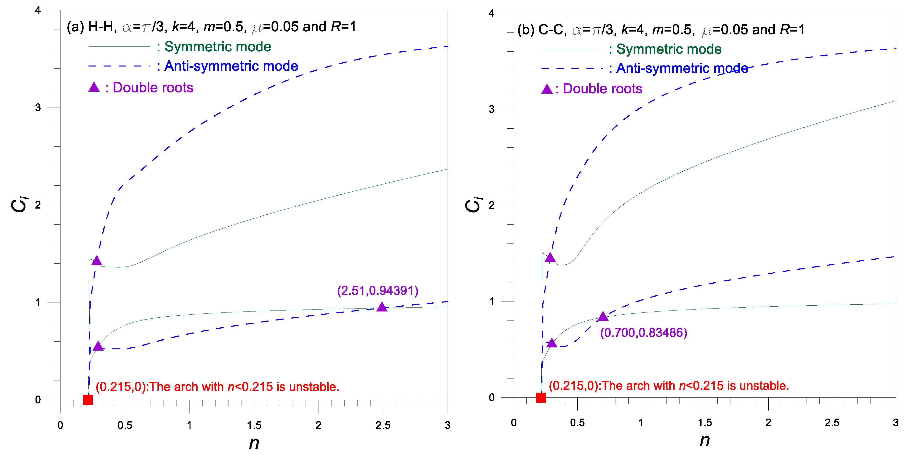
Figure 6 shows frequency curves for $C_i$ versus $n$, where $C_i$ generally increases as $n$ increases for about $n > 0.5$. However, for some of the frequency curves, $C_i$ decreases and reaches a lowest coordinates ($n,C_i$) and increases as $n$ increases for $n < 0.5$. The frequency curves in the symmetric and anti-symmetric mode intersect each other at the coordinates marked $▲$. This implies that at a single taper ratio $n$, there exists a double eigenvalue $C_i$ (i.e., the symmetric and anti-symmetric frequency parameters $C_i)$. For example, double eigenvalues $C_i$ exist at coordinates of $\left(2.51,0.94391\right)$ for $\mathrm{H}-\mathrm{H}$ arch and $\left(0.700,0.83486\right)$ for $\mathrm{C}-\mathrm{C}$ arch marked ▲. At this cross-coordinate, a mode transition occurs, which changes the mode shape from symmetric to anti-symmetric mode, and vice versa [18]. For example, in Figure 6a of $\mathrm{H}-\mathrm{H}$ arch, in the domain immediately preceding $\left(2.51,0.94391\right)$, denoted by ▲, $C_1$ is anti-symmetric and $C_2$ is symmetric, whereas in the domain immediately behind it, the mode shape order is reversed. Particularly, $C_i$ values, approaching to $0$ at $n = 0.215$ marked by ■, demonstrate that the arch with $n <0.215$ is unstable and buckles due to its self-weight without external loads or excitations. It is also observed in this figure that as the value of $n$ increases, the frequencies for C-C arches are generally higher than those for H-H arches.

Figure 7 shows the frequency curves for $C_i$ versus $\mu$, where $C_i$ increases as $\mu$ increases. The frequency curves of symmetric and anti-symmetric mode intersect each other at the coordinates marked ▲ as previously described in Figure 6. The frequencies for C-C arch are generally higher than those for H-H arches, when the value of $\mu$ are higher.

Figure 8 shows $C_i$ versus $\alpha$ curves. The $C_i$ decreases as $\alpha$ increases and the smaller $\alpha$, the steeper the rate of decrease. The frequency curves of symmetric and anti-symmetric mode intersect each other at the coordinates marked example ▲ as previously described in Figure 6.

Figure 9 shows typical examples of the mode shapes, in which the mode shapes are classified into symmetric and anti-symmetric mode. The deflections $\left(\delta ,\lambda \right)$ were initially calculated separately, but combined in a vector quantity, resulting in a deformed axis (i.e., a mode shape). In these mode shapes, the characteristics of the symmetric and anti-symmetric mode shapes are well depicted, which is represented in the conceptual diagram in Figure 3. This kind of mode shape describes the relative amplitude and the locations of maximum amplitude and nodal point, which is one of the most important data for monitoring the soundness of the arch in service.

5. Concluding Remarks

This study focused on the free vibration of the symmetric tapered circular arch made of AFGMs. Based on the dynamic equilibrium equations for an arch element, the sixth order ordinary differential equations governing the free vibration of such arch were derived. In particular, the symmetric and anti-symmetric boundary conditions at the mid-arc of the arch, not yet covered in the literature, are derived. For mathematical formulation, the quadratic polynomials are chosen as both taper and mechanical property functions. The trial eigenvalue method was used to solve these differential equations: the direct integral method of the Runge-Kutta method was used to compute the mode shapes, and the determinant search method enhanced by the Regula-Falsi method was used to compute the eigenvalues, i.e., natural frequencies. In particular, to adopt the boundary conditions, three integration intervals (the main concern of this study) were used: (a) from the left end $\left(\theta = 0\right)$ to the right end ($\theta = \alpha$), (b) from the left end $\left(\theta = 0\right)$ to the mid-arc ($\theta = \alpha /2$), and (c) from the mid-arc $\left(\theta = \alpha /2\right)$ to the right end ($\theta = \alpha$). The frequencies predicted in this study are in good agreement with those from the finite element software ADINA. The two lowest frequencies of the symmetric and anti-symmetric frequencies (i.e., totally four frequencies) were calculated. Based on the numerical experiments of this study, parametric studies on the frequencies and mode shapes are extensively discussed.

References

1. Horibe, T.; Mori, K. Large deflections of tapered cantilever beams made of axially functionally graded materials. Mech. Eng. J. JSME 2018, 5, 1–10. [Google Scholar] [CrossRef]
2. Rao, S.S. Vibration of Continuous Systems; Wiley & Sons, Inc.: New York, NJ, USA, 2007. [Google Scholar]
3. Li, X. A unified approach for analyzing static and dynamic behaviors of functionally graded Timoshenko and Bernoulli-Euler beam. J. Sound Vib. 2008, 318, 1210–1229. [Google Scholar] [CrossRef]
4. Kukla, S.; Rychlewska, J. Free vibration analysis of functionally graded beam. J. Appl. Math. Comp. Mech. 2013, 12, 39–44. [Google Scholar] [CrossRef] [Green Version]
5. Elishakoff, I.; Eisenberger, M.; Delmas, A. Buckling and vibration of functionally graded material columns sharing Duncan’s mode shape, and new cases. Structures 2016, 5, 170–174. [Google Scholar] [CrossRef]
6. Rezaiee-Pajand, M.; Masoodi, A.R. Exact natural frequencies and buckling loads of functionally graded material tapered beam-columns considering semi-rigid connections. J. Vib. Control 2018, 24, 1787–1808. [Google Scholar] [CrossRef]
7. Huang, Y.; Li, X.F. A new approach for free vibration of axially functionally graded beams with nonuniform cross-section. J. Sound Vib. 2010, 329, 2291–2303. [Google Scholar] [CrossRef]
8. Shahba, A.; Rajasekaran, S. Free vibration and stability of tapered Euler-Bernoulli beams made of axially functionally graded materials. Appl. Math. Model. 2012, 36, 3094–3111. [Google Scholar] [CrossRef] [Green Version]
9. Rajasekaran, S. Free vibration of centrifugally stiffened axially functionally graded tapered Timoshenko beams using differential transformation and quadrature methods. Appl. Math. Model. 2013, 37, 4440–4463. [Google Scholar] [CrossRef]
10. Akgoz, B.; Civalek, O. Free vibration analysis of axially functionally graded Bernoulli-Euler microbeams based on the modified couple stress theory. Compos. Struct. 2013, 98, 314–322. [Google Scholar] [CrossRef]
11. Chandran, G.; Rajendran, M.G. Study on buckling of column made of functionally graded material. Int. J. Mech. Prod. Eng. 2014, 2, 52–54. [Google Scholar]
12. Ranganathan, S.; Abed, F.; Aldadah, M.G. Buckling of slender columns with functionally graded micro-structures. Mech. Adv. Mater. Struc. 2016, 23, 1360–1367. [Google Scholar] [CrossRef]
13. Carrera, E.; Valvano, S.; Kulikov, G.M. Electro-mechanical analysis of composite and sandwich multi-layered structures by shell elements with node-dependent kinetics. Int. J. Smart Nano Mat. 2018, 9, 1–33. [Google Scholar] [CrossRef]
14. Malekzadeh, P.; Atashi, M.M.; Karami, G. In-plane free vibration of functionally graded circular arches with temperature-dependent properties under thermal environment. J. Sound Vib. 2009, 326, 837–851. [Google Scholar] [CrossRef]
15. Malekzadeh, P. Two-dimensional in-plane free vibrations of functionally graded circular arches with temperature-dependent properties. Compos. Struct. 2009, 91, 38–47. [Google Scholar] [CrossRef]
16. Rajasekaran, S. Free vibration of tapered arches made of axially functionally graded materials. Struct. Eng. Mech. 2013, 45, 569–594. [Google Scholar] [CrossRef]
17. Noori, A.R.; Aslan, T.A.; Temel, B. An efficient approach for in-plane free and forced vibrations of axially functionally graded parabolic arches with nonuniform cross section. Compos. Struct. 2018, 200, 701–710. [Google Scholar] [CrossRef]
18. Lee, J.K.; Lee, B.K. In-plane free vibration of uniform circular arches made of axially functionally graded material. Int. J. Struct. Stab. Dy. 2019, 19, 1950084. [Google Scholar] [CrossRef]
19. Weaver, W.; Timoshenko, S.P.; Young, D.H. Vibration Problems in Engineering; Wiley & Sons: New York, NJ, USA, 1990. [Google Scholar]
20. Lee, B.K.; Lee, T.E.; Choi, J.M.; Oh, S.J. Dynamic optimal arches with constant volume. Int. J. Struct. Stab. Dy. 2012, 12, 1250044. [Google Scholar] [CrossRef]
21. Timoshenko, S.P.; Gere, J.M. Mechanics of Materials; PWS Publishing Company: Boston, MA, USA, 1984. [Google Scholar]
22. Burden, R.L.; Faires, D.J.; Burden, A.M. Numerical Analysis; Cengage Learning: Boston, MA, USA, 2016. [Google Scholar]
23. Lee, J.K.; Lee, B.K. Free vibration and buckling of tapered columns made of axially functionally graded materials. Appl. Math. Model. 2019, 75, 73–87. [Google Scholar] [CrossRef]
Figure 1. Configuration of symmetric arch: (a) geometry and (b) variable functions of taper and mechanical property of AFG arch.
Symmetry 12 00417 g001
Figure 2. Loads on an arch element.
Symmetry 12 00417 g002
Figure 3. Conceptual diagram of (a) symmetric and (b) anti-symmetric boundary condition at mid-arc defined by mode shapes of ( w , v ,   M ) .
Symmetry 12 00417 g003
Figure 4. Convergence analysis.
Symmetry 12 00417 g004
Figure 5. Frequency parameter C i versus modular ratio m curves.
Symmetry 12 00417 g005
Figure 6. Frequency parameter C i versus taper ratio n curves.
Symmetry 12 00417 g006
Figure 7. Frequency parameter C i versus radial depth ratio μ curves.
Symmetry 12 00417 g007
Figure 8. Frequency parameter C i versus subtended angle α curves.
Symmetry 12 00417 g008
Figure 9. Example of mode shapes for α   =   π / 3 ,   k   =   4 ,   m   =   0.5 ,   n   =   1.2 ,   μ   =   0.05 and R   =   1 .
Symmetry 12 00417 g009