Abstract
As an effective technology for boosting the performance of wireless communications, massive multiple-input multiple-output (MIMO) systems based on symmetric antenna arrays have been extensively studied. Using low-resolution analog-to-digital converters (ADCs) at the receiver can greatly reduce hardware costs and circuit complexity to further improve the energy efficiency (EE) of the system. There are significant research on the design of MIMO detectors but there is limited study on their performance in terms of EE. This paper studies the effect of signal detection on the EE in practical systems, and proposes to apply several signal detectors based on lattice reduction successive interference cancellation (LR-SIC) to massive MIMO systems with low-precision ADCs. We report results on their achievable EE in fading environments with typical modeling of the path loss and detailed analysis of the power consumption of the transceiver circuits. It is shown that the EE-optimal solution depends highly on the application scenarios, e.g., the number of antennas employed, the cell size, and the signal processing efficiency. Consequently, the signal detector must be properly selected according to the application scenario to maximize the system EE. In addition, medium-resolution ADCs should be selected to balance their own power consumption and the associated nonlinear distortion to maximize the EE of system.
1. Introduction
Massive multiple-input multiple-output (MIMO) systems employing symmetric antenna arrays can be used to improve the spectrum efficiency (SE) of wireless communications [1,2,3,4]. In a typical massive MIMO system, analog-to-digital converters (ADCs) with symmetric quantization levels are used to convert the real and imaginary parts of the received signal before further processing. The power consumption of ADCs increases exponentially with the quantization bits. Therefore, low-precision ADCs have been widely considered recently for massive MIMO systems [5]. Significant studies have been carried out on the SE of massive MIMO with linear detectors [6,7,8,9]. In [7,10], the uplink SE of a maximum ratio combining (MRC) receiver is analyzed for massive MIMO with low-precision ADCs. The SE is analyzed for the minimum mean squared error (MMSE) receiver in [11], and it is concluded that the large arrays can compensate for the loss of low-resolution quantization. Based on the power consumption model in [3], Ref. [12] analyzes the energy efficiency (EE) of successive interference cancellation (SIC) receiver with low-precision ADCs.
Significant work has been done on the symbol detection in massive MIMO systems with low-precision ADCs. A class of techniques recover the transmitted symbols directly from the nonlinear model. In [13], iterative decision feedback receiver is studied for quantized MIMO systems. In [14], message passing dequantization (MPDQ) is applied to achieve multiuser detection for systems employing single-bit quantization. In [15], generalized approximate message passing is employed for massive MIMO with low-resolution ADCs. On the other hand, the tremendous detection algorithms designed for MIMO systems with ideal ADCs [16,17,18,19,20,21,22] can also be directly applied to quantized systems by using a linearized additive quantization noise model (AQNM). This will result in certain loss in the effective signal-to-noise ratio (SNR) but may offer solutions with moderate complexity, which are feasible for practical applications. Among the candidate techniques, the MMSE detector represents a linear option while lattice reduction-aided successive interference cancellation (LR-SIC) [23,24,25,26,27,28] provides nonlinear solutions with good tradeoff between performance and complexity for channels with large coherence blocks. The use of low-complexity, energy-efficient ADCs is also foreseen to be appealing in case of energy-constrained receive sides, such as cluster heads in massive MIMO-based wireless sensor networks (WSNs), as studied in [29,30,31,32].
In general, more advanced detectors lead to improved bit error rate (BER) performance for MIMO systems (with either ideal or low-resolution ADCs) but also higher computational complexity and higher power consumption. It is challenging to compare the different schemes and choose the one that yields the best balance between them. This work attempts to address this challenge by applying the EE as a criterion to compare several linear and nonlinear detectors. We focus on the MMSE and LR-SIC detectors due to their potential in achieving good tradeoff between performance and complexity but the work can be extended to other detectors easily. The contributions can be summarized as follows:
- We investigate the implementation of LR-SIC detectors and their improvements for massive MIMO systems with low-resolution ADCs;
- We analyze the transmission power required for achieving a target BER, the power required for signal detection, and also the power consumption due to the ADCs given the system configuration;
- We analyze and compare the EE for several different MIMO detectors under a universal system-level power consumption model, and discuss the influence of the number of antennas, the ADC resolution and also the signal processing algorithms on the performance.
Numerous numerical studies are carried out. Compared with the previous studies on MIMO detection [13,14,15,16,17,18,19,23,24,25,26,27] that focus mainly on the transmission power required, this work provides a new perspective for study the detectors in realistic scenarios under the EE criterion. Our work also differs from the previous studies on EE [3,5,12,33] where the capacity, i.e., the upper bound of the achievable rate under Gaussian signaling, is considered, as the actual power consumption for practical modulation, signal processing schemes and reliability requirement is evaluated in our studies.
The rest of this paper is organized as follows. We introduce the model of uplink large-scale massive MIMO systems with low-precision quantization in Section 2. Three MIMO detectors, i.e., MMSE, LR-SIC and a modified multi-branch LR-SIC, are then discussed in Section 3. A system-level power consumption model is introduced in Section 4, based on which the EE is analyzed. The numerical results are presented in Section 5. The conclusion is given in Section 6.
Notation: The superscripts and represent matrix inversion and transpose, respectively. denotes an identity matrix; denotes an all-zero vector of dimension . denotes expectation the determinant of . is the set of complex numbers. The notations appearing in the paper are listed in Table 1.

Table 1.
Notation.
2. System Model
In this section, we first introduce the system model of mutliuser massive MIMO systems where low-resolution ADCs are employed at the receiver. We then introduce the linearized additive quantization noise model (AQNM) that can be employed to design low-complexity signal detection algorithms.
2.1. MIMO With Low-Precision ADC
Consider an uplink single-cell scenario, where one small cell base station (BS) has N antennas serving K single-antenna users (UEs). In this case, the performance is dominated by the multiuser interference from the same cell. Following [15], we assume a Rayleigh fading channel for each coherent block, whose size depends on the coherence bandwidth and the coherent time of the channel. The received signal from all antennas are modeled as
where is the transmitted signal vector of all UEs, and has zero mean and unit power, i.e., and . The power of the UEs are specified by , in Joule/symbol represents the power allocated to the k-th user. The entries of a given column of the channel matrix , which corresponds to the channel vector of UE-k, are independent and identically distributed (i.i.d), complex Gaussian following , with being the corresponding large-scale fading for UE-k. The noise vector is additive white Gaussian noise (AWGN), in which all elements independently follow the distribution . The total transmitted SNR of the K UEs is defined as
and the received SNR of UE-k is defined as
Note that, under the i.i.d. assumption of the small scale fading of all the UEs, the BER performance of the system averaged over small-scale fading depends on . This paper assumes that the received SNRs of the different UEs are the same, achieved by reasonable power allocations according to the UEs’ large-scale fadings, as will be discussed in detail later. This amounts to assume that the UEs have symmetric requirements of quality of service (QoS) in terms of transmission rates and error rates, following [3,34,35].
In practical mobile communication systems, the elements in need to be scaled and quantized. From [36,37], the scaling factor for the n-th antenna can be chosen as
where stands for the n-th row of . Let . The received signal scales to
As illustrated in Figure 1, each antenna is equipped with two ADCs to uniformly quantize the real and imaginary parts of the signal. After quantization, the quantized received signal can be re-scaled and modeled as [15,38]
where and denote the real and imaginary part of a complex scalar, respectively. The nonlinear quantization function assumes uniform quantization with step as [39]
where we have assumed b-bit ADCs.
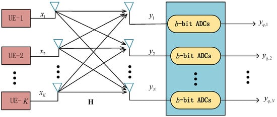
Figure 1.
Large-scale MIMO system with K UEs and N receive antennas. Each received signal is quantized by two for its real and imaginary values.
2.2. Additive Quantization Noise Model (AQNM)
Signal detection is required to recover the transmitted signal from the quantized received signal (6). The quantization introduces nonlinear distortion to the received signal, which complicates the design of optimal signal detectors. It is of interest to design suboptimal detectors which are able to achieve good tradeoff between performance and complexity. A widely used approach is to employ the AQNM [10,40] which models the quantized received signal as
where is an additive Gaussian quantization noise vector uncorrelated with and . For a fixed channel realization and given AWGN power, the covariance matrix of the quantization noise is
where is the inverse of the signal to the quantization noise ratio (SQNR) and . Following [10,15], the values of are listed in Table 2 and determined approximately by for .
Table 2.
The value of for .
3. MIMO Detection
Due to the interference among the different UEs, signal detectors are used to estimate the transmitted symbol from the quantized received signal vector modeled in (8). This is to solve an inverse problem and tremendous solutions have been studied, as surveyed in [16]. We assume that the knowledge of the channel matrix and the power of the AWGN are known at the receiver side and thus a signal detector can be constructed and reused for each coherent block. We here consider three types of detectors, i.e., the MMSE detector, the LR-SIC detector, and a modified multi-branch LR-SIC detector (MMB-LR-SIC), as example detectors of different performance and complexity. Among them, the MMSE detector is a representative linear option; the MMB-LR-SIC is adapted from the variable list detector (VLD) of [41], representing a sophisticated detector with good BER performance; and LR-SIC has complexity and performance in between MMB-LR-SIC and MMSE. The study of this paper can also be extended to other signal detectors.
3.1. MMSE Detector
Among the linear estimators, the MMSE detector achieves improved tradeoff between noise enhancement and interference cancellation by minimizing the estimation error caused by channel noise and interference [16]. Following [42], by assuming that the quantization noise is uncorrelated with the transmitted signal in (8), it can be verified that the MMSE estimator is computed as
where the covariance matrix of the quantization noise is given in (9). In order to reduce complexity and assuming i.i.d. additive quantization noise, we can approximate
where is the average power received on the antennas.
3.2. LR-SIC Detector
The LR-SIC detector represents a nonlinear detector which improves the performance by transforming the channel into a better-conditioned representation and successively canceling the interference from different UEs [23,24,26,27,43]. Consider systems with . We can first apply the QR decomposition of to reduce the computational complexity by reducing dimensions, i.e., we generate first
where
For simplicity, we assume as an AWGN with variance
We then apply the complex Lenstra-Lenstra-Lovász (CLLL) algorithm in [25] to the extended channel matrix
The LR-SIC receiver then consists of a set of linear detectors based on the lattice-reduced channel matrix
where is a unimodular matrix with . The received signal is rewritten as
with
Therefore, we can detect from first and then use the relationship in (19) to recover .
Signal detection can then be applied to the signal model (18) in the lattice-reduced domain. The MMSE-SIC algorithm [43] can be implemented using the extended received signal
and extended matrix
The estimate of can be computed successively. Assume a detector order of . With the already detected data canceled, the received signal is updated as:
Accordingly, we define a matrix as
In order to generate , MMSE estimation is applied to estimate as
where
Following [44], the estimate of is obtained by shifting and scaling the output from as
where is the i row of , denotes the rounding operator, and denote the scaling and shifting coefficients respectively, and is a vector of 1’s.
The LR-SIC can significantly improve the performance as compared with linear detection [23,24]. Compared with other nonlinear detection algorithms such as the fixed complexity sphere detector (FCSD), LR-SIC can reuse the filters and thus may exhibit a lower average complexity [43]. In the above, a natural ordering of the transmitted symbol is assumed. In fact, the order of detection can be optimized to improve performance. One option is to select the symbol that can be detected with the highest reliability at each stage. This can be based on the MMSE criterion. At the i-th stage, the MSEs achievable for detecting the un-detected symbols are given by the diagonal entries of
Therefore, we can choose the symbol that achieves the MMSE to detect at the i-th stage. The detection order obtained can be stored and reused for the whole coherence block. This is equivalent to permuting the effective channel matrix of (21) before the MMSE-SIC is performed:
where denotes the permutation matrix associated with the selected order. Accordingly, the order of the detection of the transmitted symbols should be updated.
3.3. Modified Multi-Branch LR-SIC (MMB-LR-SIC)
When the system size increases, the performance of LR-SIC still exhibits a gap to the maximum likelihood (ML) detector, as has shown in [41,43]. In [41], VLD (variable list detection) is proposed, which, in addition to the MMSE ordering-based LR-SIC as described above, also applies LR-SIC detectors with different randomly generated ordering to produce multiple estimates of the same transmitted symbol. The VLD allows the size of the candidate sets to be variable and hence the resulting complexity can vary over symbols, which can be high for certain channel uses. In this work, in order to keep the complexity tractable, we fix the number of detectors to be a finite number L. As such, random orderings are used. Denote these multiple estimates in the LR domain as , each corresponding to a specific ordering. One best estimate is selected according to the ML criterion in the LR domain [41] as
Finally, a single estimate of the transmitted symbol is generated as the output
This multi-branch approach increases the detection complexity but can noticeably improve the error performance.
4. Energy Efficiency
The detectors introduced in Section 3 have different error rate performance and complexity, which in turn affects the EE of large-scale MIMO systems with low-resolution ADCs. In this section, we first analyze the transmitted power required to achieve a fixed BER under different detection algorithms. We then analyze the corresponding receiver power consumption. Finally, we summarize the EE.
4.1. Transmission Power
Given the transmission scheme and channel statistics, the SNR required for achieving a given BER depends on the detector. Consider channels with both small-scale Rayleigh fading and large-scale fading arising from path loss. We assume that the large-scale fading between a UE and the BS antennas is the same. Following [3,33] suppose the UEs are uniformly distributed in a circular cell with radius and minimum distance
where is the distance between UE-k and the BS, and the path loss caused by UE-k due to large-scale fading is modeled as
where is the path loss exponent, and the constant regulates the channel attenuation at distance . In the channel model, the -th element in follows , where represents the path loss defined by (32) and characterizes the independent Rayleigh fading between UE-k and the n-th BS antenna. We can write
where is the Rayleigh fading component of . We assume that the target BERs for the different UEs are equal and so are the average received SNR defined in (3). Assume that is required for achieving a target BER, i.e., . Then the transmitted power is allocated according to the large-scale fading to meet the requirement. As such, the total transmission power is
where denotes the noise variance (in Joule/symbol), B is the transmission bandwidth, and denotes the total noise power.
4.2. Power Consumption by Signal Detection
We next analyze the complexity and the resulting circuit power (signal processing-related) consumption for different signal detectors. We first consider the MMB-LR-SIC detector. With MMB-LR-SIC, the overall complexity arises from the generation of multiple LR-SIC detectors per channel realization and the calculations of multiple signal estimates per channel use. The former is performed only once for a coherent interval where is fixed, while the latter is conducted for each received symbol in (6).
The power consumption of the MMB-LR-SIC at the receiver is estimated in [3,12] as
where B is the bandwidth, is the number of flops required for detection in one channel use, assuming that the detector coefficients are already computed and stored; represents the number of the calculations required to obtain to perform the QR decomposition, CLLL, filter calculations, etc, which are shared in a coherent block. represents the computational efficiency on the BS in [45]. The coefficient characterizes the number of coherence blocks (i.e., the number of times that the MMB-LR-SIC receiver is updated) in a second, which can be computed as
In the following complexity analysis, we ignore lower order terms for simplicity, which do not contribute significantly to the overall complexity. Let one flop refer to one operation of real-valued numbers, and thus each complex-valued multiplication and addition costs 6 and 2 flops, respectively. All complexity calculations are based on [46]. The QR decomposition of costs
flops. The computational complexity of the CLLL varies with channel realization and can be analyzed following [25]. In this paper, we track through numerically by summing up the complexities of the basic operations in the CLLL algorithm. Computing costs about
flops. Let be the number of columns of the extended channel matrix in (23) after the interference cancellation. Then calculating (27) costs flops and computing the filter costs about flops. Therefore, finding the K MMSE-SIC filters costs
flops, assuming that explicit inversion of is conducted. As such, the MMSE-based ordering can be achieved with no extra cost. The detector construction part requires a complexity of
In order to detect the transmitted symbol, we first calculate , which costs about flops. In the LR domain, detecting one transmitted symbol costs about flops and cancelling the interfence due to a single symbol costs another flops. After obtaining the a symbol estimate in the LR domain, computing its ML metric costs flops. Finally a single transmit symbol estimate is chose and converted to the original domain, with flops. Based on the above analysis,
which increases linearly with the number of branches L.
The LR-SIC detector is a special case of MMB-LR-SIC with . Since there is only one branch (with the MMSE ordering), there is no need to compute the ML metric. Following [3,12], its power consumption is estimated as
The computational complexity of each part is as follows:
The computational complexity of detector construction and signal detection for the three detectors is summarized in Table 3.
Table 3.
Computational complexity of signal detection and detector construction for MMB-LR-SIC, LR-SIC and MMSE detection.
4.3. ADC Power Consumption
The receiver power consumption also includes the power consumption of the ADCs. The power consumed by a single ADC is estimated by [12]
where b is the number of bits of the ADC, the figure of merit () means energy consumed per conversion step, and the sampling rate. Generally, an ADC with high-resolution leads to smaller quantization errors compared with a low-resolution ADC but also greater power consumption (48). In this paper, we assume a moderate value of fJ per conversion step [12,47] to model ADCs. Note that the power consumption due to ADC is independent of the detection algorithm applied.
4.4. Energy Efficiency
Based on the above detailed analysis of transmission power, power consumption by signal detection, and ADC power consumption, we now summarize the total power consumption of the system and calculate the system EE. Assuming quadrature phase shift keying (QPSK) signaling, i.e., one user transmits 2 bits per symbol. The total transmission rate of UE-k is . The energy efficiency is evaluated as
in , where the power consumption includes
where and denote the power consumed by a single radio frequency (RF) chain and the UE and BS, respectively; is the efficiency of the power amplifier at the transmitter; and represent the power consumption of the circuits and power amplifiers at the transmiter side; is the power consumption by signal detection, which can be evaluated as (35), (42) and (45) for the respective detectors; is the power consumed by the signal control, backhaul, etc.; is the power consumed by the local oscillator [3].
Note that the above model ignored certain power consumption such as the channel decoding, etc. However, it still provides useful insights in studying the influence of signal detection and ADC resolution on the EE. We have summarized the major steps for evaluating the EE of MIMO systems with the LR-SIC detector in Algorithm 1 and other detectors can be evaluated similarly.
| Algorithm 1 Evaluation of Energy Efficiency of MIMO Systems Employing the LR-SIC Detector |
| Input: Number of UEs K, number of receiver antennas N, radius of the cell , target BER, computational efficiency |
| Output: Energy efficiency: |
|
5. Simulation Results and Discussion
We now present numerical results with the parameter settings in Table 4, following [3,12]. QPSK modulation is assumed.
Table 4.
Simulation Parameter.
5.1. BER vs. SNR
We first compare the BER of different detection algorithms for MIMO systems low-precision ADCs. Figure 2 compares several detectors for a scenario with UEs and antennas at the BS. For the MMB-LR-SIC scheme, we set and to test detectors with different performance and complexities. In general, increasing the number of candidates L improves BER but also increases the complexity. The performance of all the detectors improve with as ADCs of higher resolutions are used, especially when the number of bits b is increased from 2 to 3. At low SNR where the noise is dominant, the difference in the BER is small for different ADCs. However, as the SNR increases, the quantization error dominates and there are significant gaps between different ADC choices. It is also clear that nonlinear signal detectors such as the LR-SIC can significantly reduce the SNR required for achieving a given BER, especially when the target BER is low and the ADC resolution is low. This indicates that more advanced symbol detectors are requried for acheiving better performance.
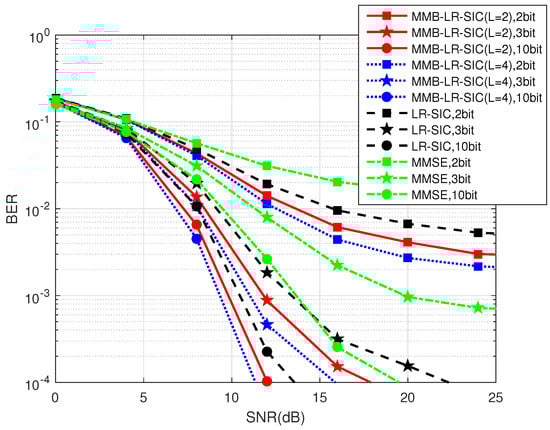
Figure 2.
BER versus the receiver SNR for .
Figure 3 compares the performance when the the number of BS antennas is increased from to 60. It is seen that the trends are similar to Figure 2. It is also interesting to see that nonlinear signal detectors still provide better performance, showing that they can improve over linear detectors even when a large number of BS antennas are employed. However, as well known from the past massive MIMO studies, the performance gaps between linear and nonlinear receivers diminishes when the condition number of the channel is improved as more antennas are used at the receiver. Meanwhile, the signal processing complexity increases when nonlinear SIC is employed as compared with the linear MMSE detector.
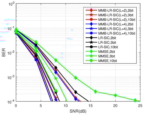
Figure 3.
BER versus the receiver SNR for .
The above SNR-BER analysis suggests that the different receivers have different error rates versus complexity tradeoff. However, it challenging to select among the different candidates. In the following, we use the EE as a performance metric to compare the different detectors under different scenarios of applications.
5.2. EE Performance
Figure 4 shows the EE performance of the different receivers with ADCs of different resolutions for and a target . It is seen that LR-SIC achieves the highest EE in general. In such a scenario, the numbers of antennas and the UEs are comparable. LR-SIC and MMB-LR-SIC can significantly reduce the transmission power required as can be seen from Figure 2. A large portion of the total power is consumed by the transmitter. The nonlinear detectors can reduce the transmitted power requirement which outweighs the increased signal processing power. As the ADC resolution improves, the EE first improves and then degrades. This is because when the resolution is too low, the transmitted power required is high; while when the resolution becomes higher, the power consumption due to the ADCs is increased. It appears that ADCs of 5 to 7 bits are advantageous.
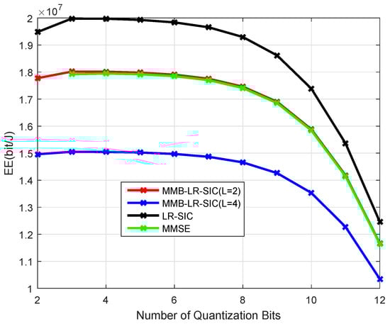
Figure 4.
Energy efficiency for , , m, at , GFlops/W.
In Figure 5, we increase the number of receiver antennas to , to consider a massive MIMO scenario. Interestingly, it is seen that in such a scenario the linear MMSE detector can be advantageous. This is because the transmission power required for achieving becomes similar for different detectors but nonlinear detectors exhibit higher signal processing complexity, which translates into higher receiver power consumption and lower EE. Also it is noted that low-resolution ADCs are advantageous when the number of antennas is large as compared with high-resolution ADCs. However, it is noticed that the overall EE degrades as compared to Figure 3 when the receiver antenna is increased from to .
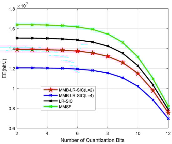
Figure 5.
Energy efficiency for , , m, at , GFlops/W.
Figure 6 shows the EE when the size of the cell is increased to 400 m for the scenario in Figure 4. Compared to Figure 4, the EE degrades due to increase of the transmission power required as the propagation loss increases on average when the cell size is increased. The relative gains provided by nonlinear LR-SIC receivers are larger in larger cells. This suggests that the nonlinear receivers may be preferred for transmissions over longer distance.
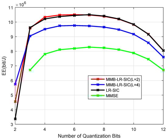
Figure 6.
Energy efficiency for , , m at , GFlops/W.
Figure 7 demonstrates the circuit power and transmission power with different numbers of quantization bits, where m and , Gflops/W. The circuit power consumption includes . It is seen that when low-resolution ADCs are used, the transmission power dominates the overall power consumption; when the number of bits increases, the circuit power consumptions become more significant. This explains the EE change in Figure 6.
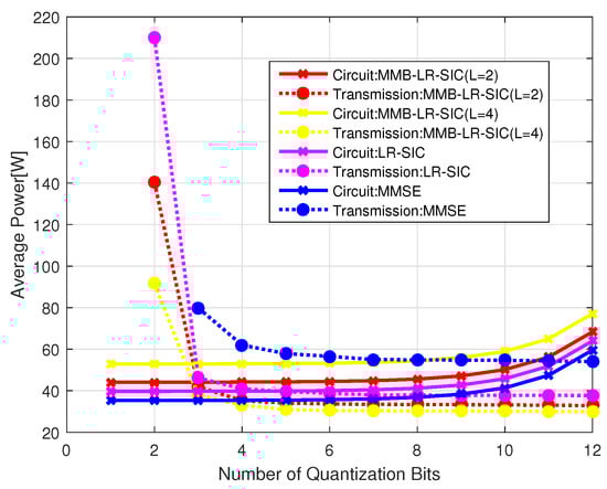
Figure 7.
Power consumption of different parts for m at GFlops/W.
Figure 8 has the same parameter as Figure 6 except . Comparing Figure 6 and Figure 8, nonlinear detectors are capable of supporting higher reliability with a higher energy efficiency, especially the LR-SIC, as compared to the MMSE detector. This is due to the relatively lower transmission power consumption for supporting a better BER. However, the advantages of nonlinear LR-SIC detector over the MMSE detector vanish when the number of BS antennas is increased. This is shown in Figure 9 where antennas are used. Furthermore, increasing the number of antennas can improve the EE as compared with Figure 8. The above results also suggest that the maximum EE is typically achieved with ADCs of intermediate resolutions, which offers good tradeoff between in the increase of transmission power due to quantization errors and the increase of the power consumptions due to ADCs themselves.
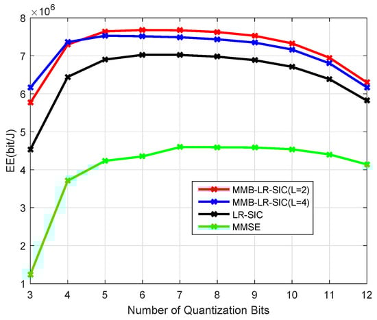
Figure 8.
Energy efficiency for m at , GFlops/W.
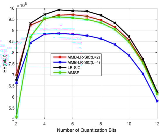
Figure 9.
Energy efficiency for with m at , GFlops/W.
Figure 10 shows the EE with m, and the computational efficiency is improved to Gflops/W. Comparing this with Figure 8, the EE is increased and similar trends are observed for the performance of different detectors.
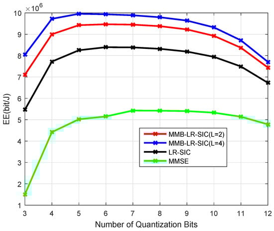
Figure 10.
Energy efficiency for m at , GFlops/W.
In Figure 11, and we consider the change of the EE with the number of receiver antennas. It is seen that the MMB-LR-SIC with has the lowest EE in the case of a large number of antennas, due to the high power consumed by signal processing, while in relatively small cells the transmission power is low for all receivers. The nonlinear receivers are advantageous when the number of BS antennas is smaller (When the number of BS antennas is small, the channel becomes more ill-conditioned. Consequently, the linear detectors based on the (pseudo)-inverse or regularized inverse of the channel matrix can introduce significant amplification of the noise. Nonlinear receivers, after interference cancellation, work on a better-conditioned channel, which results in less significant noise enhancement). In Figure 12, we can see that as computational efficiency increases, nonlinear receivers become advantageous in a larger range of cases.
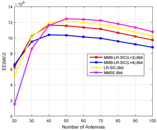
Figure 11.
Energy efficiency for UEs and 6-bit ADCs at the BS in m at , GFlops.
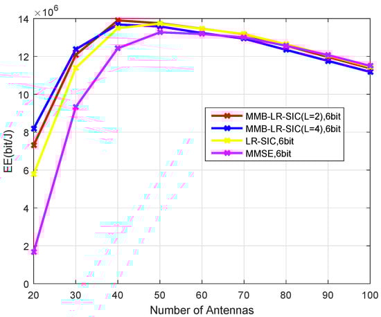
Figure 12.
Energy efficiency for UEs and -bit ADCs at the BS with m at , and GFlops/W.
6. Conclusions
In this paper, we study the detection and energy efficiency of massive MIMO systems with low-precision ADCs. The MMSE and LR-SIC detectors are studied. Their transmission power required for support a transmission rate at a given reliability is compared. The circuit power consumption including the ADCs power consumption and the signal processing complexity are analyzed. Finally, the energy efficiency with different detection algorithms under different system settings are compared. The results show that nonlinear receivers achieve better error rates but also require higher complexity. However, the EE-optimal choice of the signal detection algorithms depends highly on the concrete scenarios. In general, fewer receiver antennas, higher reliability requirement, larger cell size may require nonlinear detectors to be used to achieve the highest EE. While the linear detector may be more advantageous when the transmission power required is low, such as when the number of BS antennas is large, cell size is small, etc.
It should be noted that the framework presented in this paper can be adapted to analyze systems based on different modulation schemes (e.g., multiple-PSK (M-PSK), multiple- Quadrature Amplitude Modulation (M-QAM)), signal detectors, channel models, transceiver architectures, and power allocation schemes, by characterizing the error rate performance and computational complexity of the detector concerned. Other future work may include the extension to multiple-cell scenarios and wireless sensor networks.
Author Contributions
Conceptualization, Z.X., L.G.; methodology, Z.X., J.Z., T.L.; software, J.Z., L.G.; validation, J.T., T.L.; formal analysis, J.Z., J.T.; investigation, J.Z.; resources, Z.X., L.G.; data curation, J.Z.; writing–original draft preparation, J.Z., J.T.; writing–review and editing, Z.X., T.L., F.Z., J.T.; visualization, J.Z., J.T.; supervision, Z.X., L.G., F.Z.; project administration, Z.X., L.G., F.Z.; funding acquisition, Z.X., F.Z., J.T. All authors have read and agreed to the published version of the manuscript.
Funding
This research was funded by NSFC under Grant 61601325.
Conflicts of Interest
The authors declare no conflict of interest.
References
- Marzetta, T. Noncooperative cellular wireless with unlimited numbers of base station antennas. IEEE. Trans. Wirel. Commun. 2010, 9, 3590–3600. [Google Scholar] [CrossRef]
- Rusek, F.; Persson, D.; Lau, B.K.; Larsson, E.G.; Marzetta, T.L.; Edfors, O.; Tufvesson, F. Scaling up MIMO: Opportunities and challenges withvery large arrays. IEEE Signal. Proc. Mag. 2013, 30, 40–60. [Google Scholar] [CrossRef]
- Björnson, E.; Sanguinetti, L.; Hoydis, J.; Debbah, M. Optimal design of energy-efficient multi-user MIMO systems: Is massive MIMO the answer? IEEE. Trans. Wirel. Commun. 2015, 6, 3059–3075. [Google Scholar] [CrossRef]
- Björnson, E.; Larsson, E.G.; Marzetta, T.L. Massive MIMO: Ten myths and one critical question. IEEE. Commun. Mag. 2016, 54, 114–123. [Google Scholar] [CrossRef]
- Bai, Q.; Nossek, J.A. Energy efficiency maximization for 5G multi-antenna receivers. Trans. Emergy Telecommun. Technol. 2015, 26, 3–14. [Google Scholar] [CrossRef]
- Zhang, J.; Dai, L.; He, Z.; Jin, S.; Li, X. Performance analysis of mixed-ADC massive MIMO systems over Rician fading channels. IEEE J. Sel. Areas Commun. 2017, 35, 1327–1338. [Google Scholar] [CrossRef]
- Zhang, J.; Dai, L.; Sun, S.; Wang, Z. On the spectral efficiency of massive MIMO systems with low-resolution ADCs. IEEE Commun. Lett. 2016, 20, 842–845. [Google Scholar] [CrossRef]
- Jacobsson, S.; Durisi, G.; Coldrey, M.; Gustavsson, U.; Studer, C. Throughput analysis of massive MIMO uplink with low-resolution ADCs. IEEE Trans. Wirel. Commun. 2017, 16, 4038–4051. [Google Scholar] [CrossRef]
- Mo, J.; Heath, R.W. Capacity analysis of one-bit quantized MIMO systems with transmitter channel state information. IEEE Signal. Proc. Mag. 2015, 63, 5498–5512. [Google Scholar] [CrossRef]
- Fan, L.; Jin, S.; Wen, C.-K.; Zhang, H. Uplink achievable rate for massive MIMO systems with low-resolution ADC. IEEE Commun. Lett. 2015, 19, 2186–2189. [Google Scholar] [CrossRef]
- Dong, Y.; Qiu, L. Spectral efficiency of massive MIMO systems with low-resolution ADCs and MMSE receiver. IEEE Commun. Lett. 2017, 21, 1771–1774. [Google Scholar] [CrossRef]
- Liu, T.; Tong, J.; Guo, Q.; Xi, J.; Yu, Y.; Xiao, Z. Energy efficiency of massive MIMO systems with low-resolution ADCs and successive interference cancellation. IEEE Trans. Wirel. Commun. 2019, 18, 3987–4002. [Google Scholar] [CrossRef]
- Azizzadeh, A.; Mohammadkhani, R.; Makki, S. BER performance of uplink massive MIMO with low-resolution ADCs. In Proceedings of the IEEE 2017 7th International Conference on Computer and KnowledgeEngineering (ICCKE), Mashhad, Iran, 26–27 October 2017; pp. 298–302. [Google Scholar]
- Wang, S.; Li, Y.; Wang, J. Multiuser detection for uplink large-scale MIMO under one-bit quantization. In Proceedings of the 2014 IEEE International Conference on Communications (ICC), Sydney, Australia, 10–14 June 2014; pp. 4460–4465. [Google Scholar]
- Xiong, Y.; Wei, N.; Zhang, Z. A Low-Complexity Iterative GAMP-Based Detection for Massive MIMO with Low-Resolution ADCs. In Proceedings of the 2017 IEEE Wireless Communications and Networking Conference (WCNC), San Francisco, CA, USA, 19–22 March 2017; pp. 1–6. [Google Scholar]
- Yang, S.; Hanzo, L. Fifty years of MIMO detection: The road to large-scale MIMO. IEEE Commun. Surv. Tutor. 2015, 17, 1941–1988. [Google Scholar] [CrossRef]
- Jalden, J.; Ottersten, B. On the complexity of sphere decoding in digital communications. IEEE Signal. Proc. Mag. 2005, 53, 1474–1484. [Google Scholar] [CrossRef]
- Wang, Y.; Wang, J.-k.; Song, X.; Xie, Z.-B. Mmse V-Blast algorithm basedon iterative QR decomposition. J. Northeastern. Univ. 2008, 29, 65–68. [Google Scholar]
- Barbero, L.G.; Thompson, J.S. Fixing the complexity of the sphere decoder for MIMO detection. IEEE Trans. Wirel. Commun. 2008, 7, 2131–2142. [Google Scholar] [CrossRef]
- Kim, T.-H. Low-complexity sorted QR decomposition for MIMO systems based on pairwise column symmetrization. IEEE Trans. Wirel. Commun. 2014, 13, 1388–1396. [Google Scholar] [CrossRef]
- Tong, J.; Schreier, P.J.; Weller, S.R. Design and analysis of largeMIMO systems with Krylov subspace receivers. IEEE Trans. Signal. Proc. 2012, 60, 2482–2493. [Google Scholar] [CrossRef]
- Mezghani, A.; Rouatbi, M.; Nossek, J.A. An iterative receiver for quantized MIMO systems. In Proceedings of the 2012 16th IEEE Mediterranean Electrotechnical Conference, Yasmine Hammamet, Tunisia, 25–28 March 2012; pp. 1049–1052. [Google Scholar]
- Yao, H.; Wornell, G.W. Lattice-reduction-aided detectors for MIMO communication systems. In Proceedings of the IEEE Global Telecommunications Conference, Taipei, Taiwan, 17–21 November 2002; pp. 424–428. [Google Scholar]
- Wubben, D.; Bohnke, R.; Kuhn, V.; Kammeyer, K.D. Near-maximum-likelihood detection of MIMO systems using MMSE-based lattice reduction. In Proceedings of the IEEE International Conference on Communications, Paris, France, 20–24 June 2004; pp. 798–802. [Google Scholar]
- Gan, Y.H.; Ling, C.; Mow, W.H. Complex lattice reduction algorithm for low-complexity full-diversity MIMO detection. IEEE Signal. Proc. Mag. 2009, 57, 2701–2710. [Google Scholar]
- Shabany, M.; Gulak, P.G. The application of lattice-reduction to the K-best algorithm for near-optimal MIMO detection. In Proceedings of the 2008 IEEE International Symposium on Circuits and Systems (ISCAS), Seattle, WA, USA, 18–21 May 2008; pp. 316–319. [Google Scholar]
- Arevalo, L.; Lamare, R.C.; Zu, K.; Sampaio-Neto, R. Multi-branch lattice reduction successive interference cancellation detection for multiuser MIMO systems. In Proceedings of the 2014 11th International Symposium on Wireless Communications Systems (ISWCS), Barcelona, Spain, 26–29 August 2014; pp. 219–223. [Google Scholar]
- Zhou, Q.; Ma, X. Element-based lattice reduction algorithms for large MIMO detection. IEEE J. Sel. Areas Commun. 2013, 31, 274–286. [Google Scholar] [CrossRef]
- Chawla, A.; Patel, A.; Jagannatham, A.K.; Varshney, P.K. Distributed Detection in Massive MIMO Wireless Sensor Networks Under Perfect and Imperfect CSI. IEEE Trans. Signal Process. 2019, 67, 4055–4068. [Google Scholar] [CrossRef]
- Ciuonzo, D.; Rossi, P.S.; Dey, S. Massive MIMO Channel-Aware Decision Fusion. IEEE Trans. Signal Process. 2015, 63, 604–619. [Google Scholar] [CrossRef]
- Ding, G.; Gao, X.; Xue, Z.; Wu, Y.; Shi, Q. Massive MIMO for Distributed Detection With Transceiver Impairments. IEEE Veh. Technol. 2018, 67, 604–617. [Google Scholar] [CrossRef]
- Ciuonzo, D.; Romano, G.; Rossi, P.S. Performance Analysis and Design of Maximum Ratio Combining in Channel-Aware MIMO Decision Fusion. IEEE Trans. Wirel. Commun. 2013, 12, 4716–4728. [Google Scholar] [CrossRef]
- Liu, T.; Tong, J.; Guo, Q.; Xi, J.; Yu, Y.; Xiao, Z. Energy efficiency of uplink massive MIMO systems with successive interference cancellation. IEEE Commun. Lett. 2017, 21, 668–671. [Google Scholar] [CrossRef]
- Sanguinetti, L.; Moustakas, A.L.; Debbah, M. Interference management in 5G reverse TDD HetNets with wireless backhaul: A large system analysis. IEEE J. Sel. Areas Commun. 2015, 33, 1187–1200. [Google Scholar] [CrossRef]
- Sanguinetti, L.; Moustakas, A.L.; Bjornson, E.; Debbah, M. Large system analysis of the energy consumption distribution in multi-user MIMO systems with mobility. IEEE Trans. Wirel. Commun. 2015, 14, 1730–1745. [Google Scholar] [CrossRef]
- Gray, R.M.; Neuhoff, D.L. Quantization. IEEE Trans. Inform. Theory 1998, 44, 2325–2383. [Google Scholar] [CrossRef]
- Abbas, W.; Gomez-Cuba, F.; Zorzi, M. Millimeter wave receiver efficiency: A comprehensive comparison of beamforming schemes with low resolution ADCs. IEEE Trans. Wirel. Commun. 2017, 16, 8131–8146. [Google Scholar] [CrossRef]
- Moon, S.; Kim, I.; Kam, D.; Jee, D.; Choi, J.; Lee, Y. Massive MIMO systems with low-resolution ADCs: Baseband energy consumption vs. symbol detection performance. IEEE Access. 2019, 7, 6650–6660. [Google Scholar] [CrossRef]
- Wang, S.; Li, Y.; Wang, J. Multiuser Detection in Massive Spatial Modulation MIMO With Low-Resolution ADCs. IEEE Trans. Wirel. Commun. 2015, 14, 2156–2168. [Google Scholar] [CrossRef]
- Tan, W.; Jin, S.; Wen, C.; Jing, Y. Spectral efficiency of mixed-ADC receivers for massive MIMO systems. IEEE Access. 2016, 4, 7841–7846. [Google Scholar] [CrossRef]
- Arevalo, L.; Lamare, R.C.; Sampaio-Neto, R. Variable list detection for multiuser MIMO systems. IEEE Trans. Veh. Technol. 2017, 66, 3012–3023. [Google Scholar] [CrossRef]
- Kay, S.M. Fundamentals of Statistical Signal Processing: Est Imat ion Theory; University of Rhode Island: South Kingstown, Rhode Island, 1993. [Google Scholar]
- Tong, J.; Guo, Q.; Xi, J.; Yu, Y.; Schreier, P.J. Regularized lattice reduction-aided ordered successive interference cancellation for MIMO detection. In Proceedings of the 2018 IEEE Statistical Signal Processing Workshop (SSP), Freiburg, Germany, 10–13 June 2018; pp. 10–13. [Google Scholar]
- Milford, D.; Sandell, M. Simplified Quantisation in a Reduced-Lattice MIMO Decoder. IEEE Commun. Lett. 2011, 15, 725–727. [Google Scholar] [CrossRef]
- Björnson, E. Emil and Hoydis, Jakob and Sanguinetti, Luca. Massive MIMO Networks: Spectral, Energy, and Hardware Efficiency. Found. Trends Signal Process. 2017, 11, 154–655. [Google Scholar] [CrossRef]
- Hunger, R. Floating Point Operations in Matrix-Vector Calculus; Inst. for Circuit Theory and Signal Processing; Tech. Rep. TUM-LNS-TR-05-05; Munich University of Technology: Munich, Germany, 2005. [Google Scholar]
- Murmana, B. ADC Performance Survey 1997–2017. Available online: http://web.standford.edu/murmann/adcsurvey.html (accessed on 20 December 2019).


© 2020 by the authors. Licensee MDPI, Basel, Switzerland. This article is an open access article distributed under the terms and conditions of the Creative Commons Attribution (CC BY) license (http://creativecommons.org/licenses/by/4.0/).