Article

A Clinical Decision-Support System Based on Three-Stage Integrated Image Analysis for Diagnosing Lung Disease

1
Department of Information Management, National Yunlin University of Science & Technology, Yunlin 64002, Taiwan
2
Department of Digital Content Applications and Management, Wenzao Ursuline University of Languages, Kaohsiung 80793, Taiwan
*
Author to whom correspondence should be addressed.
Symmetry 2020, 12(3), 386; https://doi.org/10.3390/sym12030386
Submission received: 13 February 2020 / Revised: 27 February 2020 / Accepted: 1 March 2020 / Published: 3 March 2020

Abstract

:
Thoracic computed tomography (CT) technology has been used for lung cancer screening in high-risk populations, and this technique is highly effective in the identification of early lung cancer. With the rapid development of intelligent image analysis in the field of medical science and technology, many researchers have proposed computer-aided automatic diagnosis methods for facilitating medical experts in detecting lung nodules. This paper proposes an advanced clinical decision-support system for analyzing chest CT images of lung disease. Three advanced methods are utilized in the proposed system: the three-stage automated segmentation method (TSASM), the discrete wavelet packets transform (DWPT) with singular value decomposition (SVD), and the algorithms of the rough set theory, which comprise a classification-based method. Two collected medical CT image datasets were prepared to evaluate the proposed system. The CT image datasets were labeled (nodule, non-nodule, or inflammation) by experienced radiologists from a regional teaching hospital. According to the results, the proposed system outperforms other classification methods (trees, naïve Bayes, multilayer perception, and sequential minimal optimization) in terms of classification accuracy and can be employed as a clinical decision-support system for diagnosing lung disease.

1. Introduction

In recent years, substantial difficulties have been encountered in the treatment of lung cancer, which have attracted increasing attention in medical research. Since 2008, according to medical statistics, lung cancer has been the cancer with the highest mortality rate. If lung cancer could be diagnosed in its initial stage, the 5-year survival probability of patients would increase to 70% [1]. Therefore, the early diagnosis of lung cancer generally increases the chances for successful treatment. Thoracic computed tomography (CT) is a highly effective tool that facilitates the diagnosis of lung metastases in tumor patients and the assessment of the progression of lung tumors during their treatment. With improvements in CT scanners and image analysis methods, the diagnostic sensitivity of pulmonary nodules has also improved [2,3]. In recent years, CT technology has been used for lung cancer screening in high-risk populations, and this technique is highly effective in the identification of early lung cancer [4].
Since chest CT technology is mainly utilized for the diagnosis of lung disease, medical specialists must spend substantial time and effort analyzing numerous chest CT slices. As a result, expert fatigue is considered a limitation in the early diagnosis of lung diseases. Moreover, interreader variability occurs in the detection of lung nodules by medical specialists [5]. To improve the current CT examination mechanisms, many CT imaging analysis methods have been proposed for aiding doctors in diagnosing lung diseases. Based on the reviewed literature, we argue that past automatic pulmonary nodule detection methods can be roughly classified into three types: classification-based, template-based, and segmentation-based methods. Of these three types, classification-based methods perform the best [6]. Moreover, most of the previous automatic methods for detecting pulmonary nodules involve techniques for scanning lung and nodule contours. For example, Mullaly et al. (2002) provided an approach for utilizing the location, shape, nodule size, and exclusivity measures to match nodules [7]. Dehmeshki et al. (2007) presented a method for distinguishing nodules from their adjoining blood vessels according to the volumetric shape index of each voxel and a 3D geometric feature [8]. Yeny et al. (2008) applied a technique based on a scan line search for smoothing lung boundaries [9].
After reviewing the literature, we have identified two major issues that are encountered by the available methods and have proposed corresponding solutions accordingly. Firstly, the segmentation of clear lung areas (regions of interest, ROIs) in initial CT images is crucial for medical image specialists because such areas provide strong diagnostic evidence for lung disease. Therefore, we believe that an intelligent image segmentation method should be able to clearly outline ROIs as a basis for disease diagnosis. Secondly, high accuracy is necessary for a computer-based clinical system. However, the traceability of diagnosis results is rarely discussed in the literature. We argue that an advanced clinical support system should be able to produce high-accuracy diagnostic results with traceable rules. Such a system would be more likely to be trusted by doctors and medical image specialists than systems without such rules.
Hence, this paper proposes a clinical decision-support system based on three advanced image analysis and classification methods for facilitating the diagnosis process and improve accuracy: (1) a three-stage automated segmentation method (TSASM) for outlining the ROI, (2) a discrete wavelet packet transform (DWPT) with singular value decomposition (SVD) [10,11,12] for extracting the image features of the ROI, and (3) the rough set theory (RST) [13,14,15,16] as a classification method for the classification and diagnosis of pulmonary diseases based on chest CT images.

2. Related Works

In the following sections, related studies on singular value decomposition, discrete wavelet packet transform, and rough sets are briefly introduced.

2.1. Singular Value Decomposition (SVD)

The singular value decomposition (SVD) method is a matrix factorization technique [12] for image analysis. The method is introduced briefly in this section. SVD can reduce a high-rank matrix to a low-rank matrix while preserving important information. Thus, SVD is a dimension reduction method. Supposing the input image is represented by a M × N matrix A with rank r . Via SVD, matrix A can be decomposed as follows [17]
A = U D V T = [ u 1 , 1 u 1 , M u 2 , 1 u 2 , M u M , 1 u M , M ] [ d 1 0 0 d 2 0 0 0 0 d r ] [ v 1 , 1 v 1 , N v 2 , 1 v 2 , N v N , 1 v N , N ] T
where U and V are orthogonal matrices whose dimensions are M × M and   N × N , respectively, and D , which is called the singular matrix, is an M × N diagonal matrix whose diagonal entries are nonnegative real numbers.

2.2. Discrete Wavelet Packet Transform (DWPT)

The wavelet transform (WT) method has been applied in various fields, such as telecom, the target recognition of radars, and the image classification of textures [11]. The main advantage of the wavelet transform method is that it can be applied to various window sizes and to slow and fast frequencies [18]. Since the window can adapt to the transient state of each scale, the wavelet transform method does not require a “stationarity” condition to be satisfied [19,20].
In the traditional approach, the discrete wavelet transform (DWT) method can only recursively decompose low-frequency bands. However, some high-frequency bands should also be decomposed to obtain additional information. The DWPT is an extension of the DWT and enables both detail and approximation results to be decomposed further, therefore this method can use low-pass filter and high-pass filter collections to decompose more detailed coefficients. In 1-level wavelet packet decomposition, the cell of ‘L-L1’ is an approximation and the other three cells (‘L-H1’, ‘H-L1’, and ‘H-H1’) are the detail results. In 2-level wavelet packet decomposition, the cell of ‘L-L2’ is an approximate result, and the other 15 cells are detail results. The main advantage of DWPT is that it can combine various levels of decomposition to generate the optimal time-frequency representation of an original source [21].
The standard 2D-DWPT method can be applied in a low-pass filter h and a high-pass filter [16]. The 2D-DWPT of an N × M discrete image X up to level p + 1 ( p m i n ( log 2 N , log 2 M ) ) is defined, along with the coefficients at level p , by the following Equations (1)–(4) [22]
C 4 k , ( i ,   j ) p + 1 = m n h ( m ) h ( n ) C k , ( m + 2 i ,   n + 2 j ) p
C 4 k + 1 , ( i ,   j ) p + 1 = m n h ( m ) g ( n ) C k , ( m + 2 i ,   n + 2 j ) p
C 4 k + 2 , ( i ,   j ) p + 1 = m n g ( m ) h ( n ) C k , ( m + 2 i ,   n + 2 j ) p
C 4 k + 3 , ( i ,   j ) p + 1 = m n g ( m ) g ( n ) C k , ( m + 2 i ,   n + 2 j ) p
where C 0 , ( i ,   j ) 0 is image X , and in each step, image C k p is decomposed into four quarter-sized images, namely, C 4 k p + 1 , C 4 k + 1 p + 1 ,   C 4 k + 2 p + 1 , C 4 k + 3 p + 1 , as illustrated in Figure 1.
An orthonormal wavelet basis is selected; the computed coefficients are independent, with a distinct feature of the original signal [23]. According to Muneeswaran et al. [23], wavelet packets can be represented by basic functions, as in Equations (5) and (6):
W 2 n ( 2 p 1 x 1 ) = 2 l p m h ( m 2 l ) 2 p W n ( 2 p x m )
W 2 n + 1 ( 2 p 1 x 1 ) = 2 l p m g ( m 2 l ) 2 p W n ( 2 p x m )
where p denotes a scale index, l represents a translation index, h is a low-pass filter, g is a high-pass filter, and   g ( k ) = ( 1 ) k h ( 1 k ) . The function W 0 ( x ) is a scaling function Φ , and W 1 ( x ) has the mother wavelet   Ψ .

2.3. Rough Sets Theory

Pawlak (1982) proposed the rough sets for extracting rules from a large number of instances to support decision making [13]. This theory can be regarded as a new mathematical approach to vagueness [15]. The theory of “rough sets” is based on the assumption that every object is associated with some information (knowledge). For example, while an object is a manifestation of a patient with a disease, information is only a symptom of the disease. Jothi et al. (2016) proposed a TRSFFQR (tolerance rough set firefly-based quick reduct) for selecting features, and applied it to MRI brain images [16]. The effectiveness of the rough sets in the area of medical CT image analysis has been proven. For an introduction to the concept of rough sets, refer to the related literature [13,14,15].
The rough sets method is used to analyze information system (IS) via a series of logical inference processes. An I S can be regarded as a decision table that is denoted by I S = ( U ,   A ,   C ,   D ) , in which U is the universe of discourse and A is a set that consists of primitive features (characters or variables). Let A = C D , C D = , and   C , D A be two subsets of features, where C is a “condition feature” and D denotes a decision feature. The inexactness of an approximation classification is defined as the quality of the approximation of X   by   B . This refers to the percentage of objects that are correctly classified into class X using the feature B [13]. The quality of the classification accuracy is defined in Equation (7)
γ B ( A ) = c a r d ( B _ X i ) c a r d ( U )
If   γ B ( A ) = 1 , the decision table is consistent; otherwise, it is not consistent.
Feature reduction is an important task in rough sets, in which the set of reduced features can realize the same quality of approximation as the original full set of features. Using feature reduction, rules can be generated for determining the values of a decision feature based on the values of condition features; the rules are represented as “IF condition(s) THEN decision(s)”.

3. Materials and Proposed System

3.1. Medical Image Datasets

In this research, two medical image datasets were prepared to evaluate the proposed system. One was collected from the lung image database consortium (LIDC), and the other was obtained from a regional teaching hospital (RTH) in Taiwan.

3.1.1. LIDC Image Dataset

The LIDC dataset was collected from five sites in the United States [24]. The LIDC dataset is formatted as DICOM and has a high resolution and sensitivity to chest anatomy. The dataset is composed of 100 chest CT images. The images come from patients of different genders, ages and case histories. In addition, the 100 chest images were evaluated by three experienced radiologists from a regional teaching hospital in Taiwan and labeled with three categories: nodule, non-nodule, and inflammation.

3.1.2. RTH Image Dataset

The RTH dataset was collected by the same process as the LIDC dataset and contains 100 CT images. Three radiologists participated in this research and gave evaluation results (nodule or non-nodule) for the 100 images contained in the RTH image dataset. Nodules located in the central and peripheral areas of the CT image are labeled with “nodule”. The image format for the RTH dataset is “JPG”. Although its resolution is lower than that of the LIDC dataset, we believe that this will not impact the analysis results of the human anatomical images.

3.2. Proposed System

In this paper, we have proposed an advanced clinical decision-support system based on the three proposed methods: the three-stage automated segmentation method (TSASM), the discrete wavelet packets transform (DWPT) with singular value decomposition (SVD), and rough set algorithms. The framework of the proposed system is illustrated in Figure 2. The system has four processing blocks, which are introduced briefly in the following.

3.2.1. Image Processing Block (A)

In this block, chest CT images are preprocessed with two sub-processes as follows: (1) adjusting the image contrast: adjusting the image contrast based on the density difference between the lung and thoracic cavity areas; and (2) outlining the lung areas from a chest CT image—outline the lung areas of a chest CT image with a box field by the three-stage automated segmentation method (TSASM) and the region-growing method (RGM) [25,26].

3.2.2. Reconstruction Block (B)

This block applies the SVD method to compute the singular values for the processed lung image from block (A); these values will be utilized in the reconstruction of the lung areas in the chest CT image in the next block.

3.2.3. Feature Extraction Block (C)

This block consists of two sub-processes: (1) The process of image construction with the wavelet packet coefficients for the chest CT image and two reconstruction methods (DWPT and DWPT with SVD) are provided in this block to analyze the chest CT image with wavelet packet coefficients; and (2) employ the “reduct sets” from the rough set theory to select wavelet packet features and reduce the features of the chest CT image.

3.2.4. Classification Block (D)

In this block, the algorithms of the rough set theory (LEM2) [27] are employed to generate understandable rules for medical image specialists by extracting and classifying the two image datasets (reconstructed and non-reconstructed with SVD), which have been processed previously by the DWPT method in block (C).

3.3. Proposed Procedure

The procedure of the proposed system is composed of six steps: (1) adjusting the image contrast, (2) outlining the lung area, (3) reconstructing the image by SVD, (4) generating a coefficient by DWPT, (5) computing the feature values and reducing features, and (6) classifying the lung image dataset. The detailed steps are introduced as follows.
Step 1: Adjusting Image Contrast
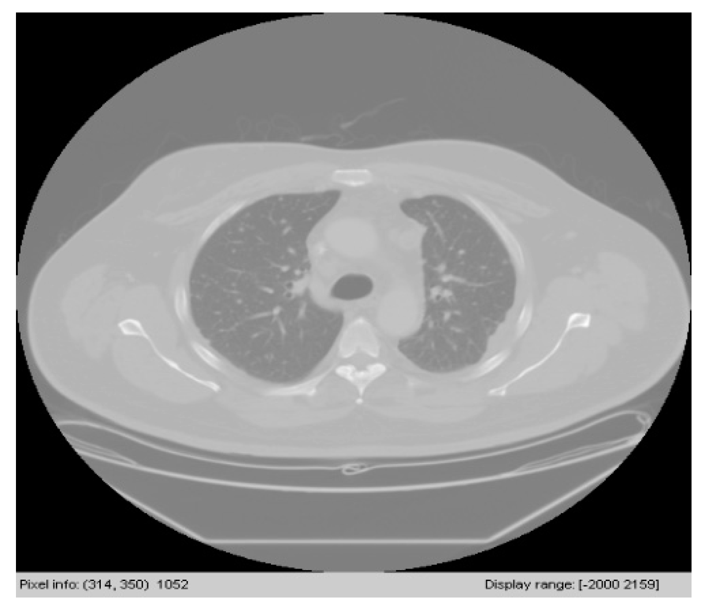
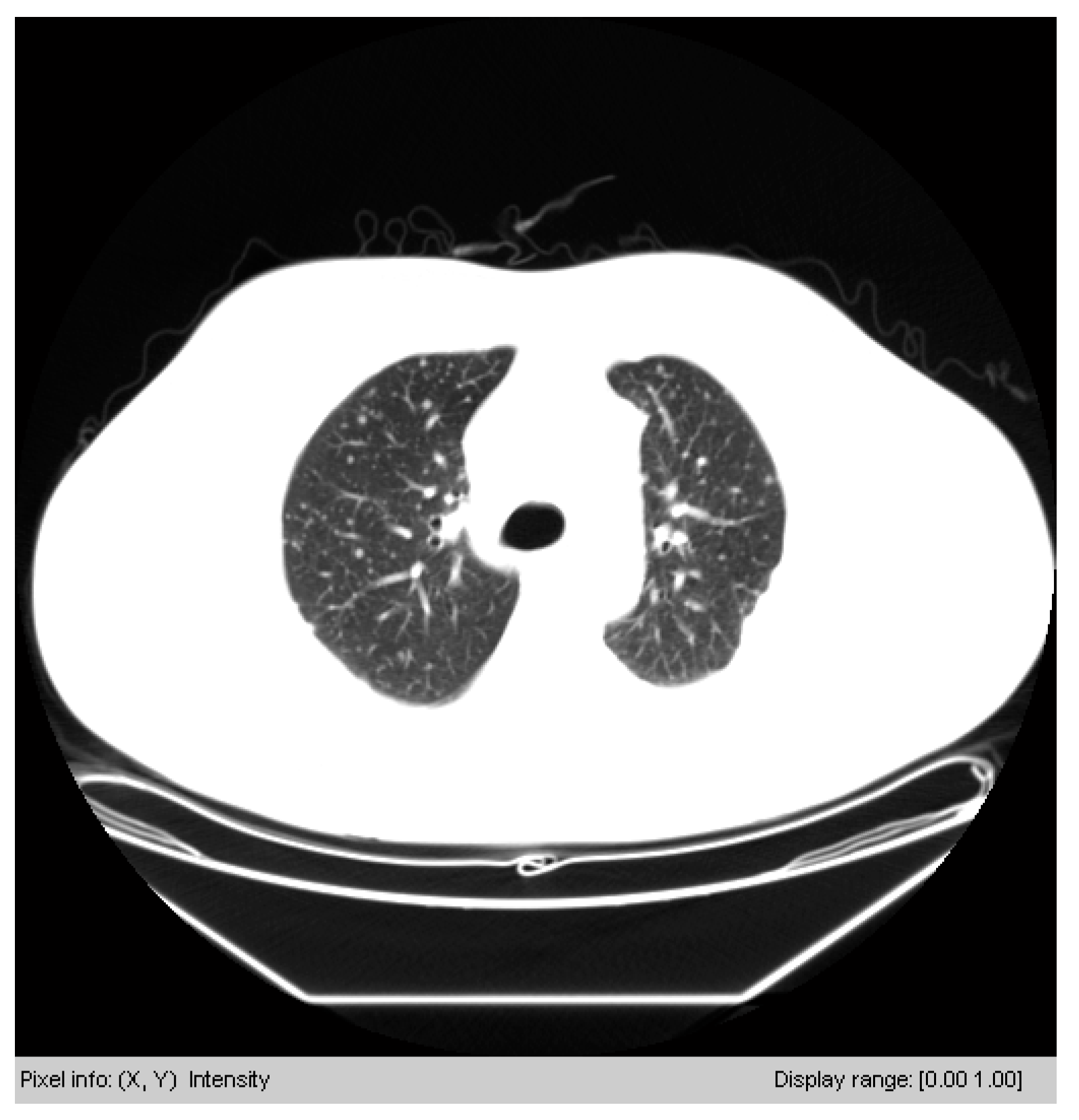
The contrast of an original medical image is sometimes insufficient (see Figure 3). An adjustment process is required for original medical images and is performed in the proposed system. We use the LIDC image dataset to demonstrate this process with two steps.
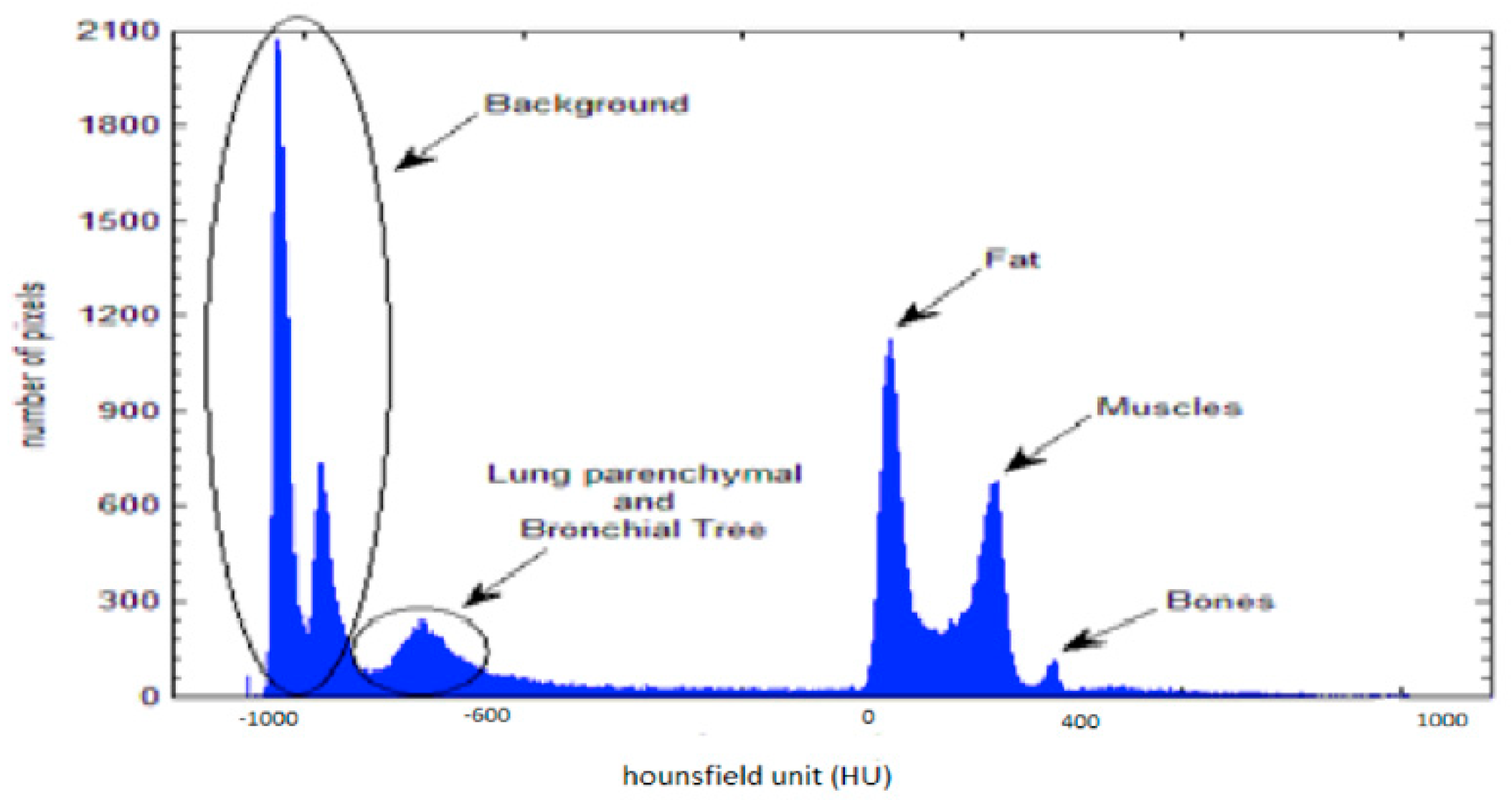
Firstly, the original medical image is automatically adjusted by the contrast adjustment tool to produce a clear image with a high contrast (see Figure 4) and to generate a histogram of its strength (see Figure 5). The chest CT images have two main density distribution areas: (1) low-density areas, representing the background air, lungs, and bronchial trees; and (2) high-density areas, representing fats, muscles, and bones.
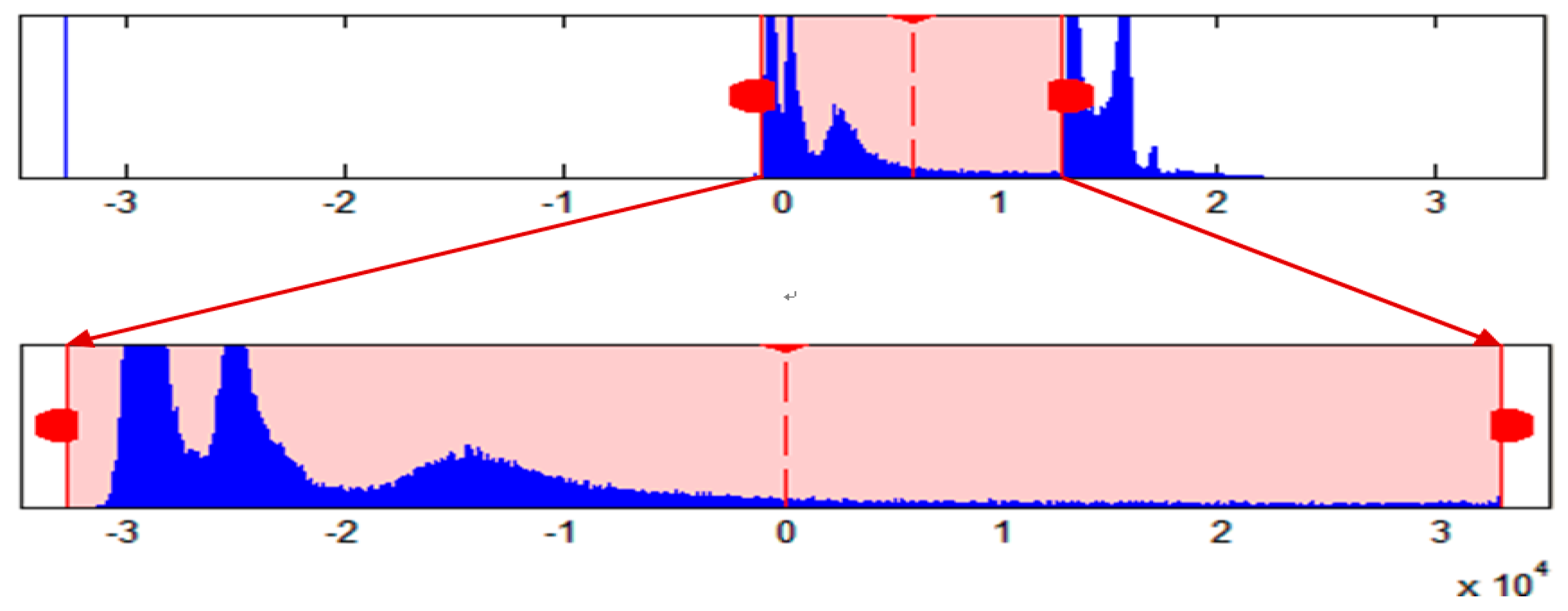
Secondly, the adjusted image from the above process (see Figure 5) is tuned again, with its contrast as follows. The display range for the image is set from the starting point of the ‘background’ and the end point before the ‘fat’, and the selected range (from the ‘background’ to ‘fat’) is expanded to the whole pixel range (the whole range is from −32,768 to 32,767 with an integer type). Figure 6 illustrates the tuning process for expanding the display range. After this process, the high-density areas (representing fats, muscles, and bones) are shown with one density (a white color) and excluded from the image display (see Figure 7).
Step 2: Outlining the Lung Area
To clearly refine the region of interest (ROI), an image segmentation method is proposed in this system (a three-stage automated segmentation method (TSASM)) to outline the lung areas with a box field. Figure 8 demonstrates the image processing processes of the proposed method. Each stage of this method is introduced as follows.

3.3.1. Segmenting the Chest CT Image

With this process, we can remove most of the irrelevant areas from the chest CT image from Step 1. Figure 9 illustrates the unprocessed and processed images. The algorithm of this process is listed as Algorithm 1.
Algorithm 1: Segmenting chest CT image
Input: image I (size of I is 512 × 512)
begin
   for i ⃪ 1 to 512 do
   if j = 1 512 I ( i ,   j ) > T c h e s t
    x = i break
   end
   end
for j ⃪ 1 to 512 do
   if i = 1 512 I ( i ,   j ) > T c h e s t
    y = j break
   end
   end
for i ⃪ 512 to 1 do
   if j = 1 512 I ( i ,   j ) > T c h e s t
    W = i break
   end
   end
for j ⃪ 512 to 1 do
   if i = 1 512 I ( i ,   j ) > T c h e s t
    H = j break
   end
   end
end
Output: image I crop from I ( x , y ) , width is W-x, and height is H-y

3.3.2. Removing Irrelevant Background Areas

With this process, we can remove the irrelevant background areas of the CT image and save the lung regions for further diagnostic analysis. Figure 10 demonstrates the unprocessed and processed images. The algorithm for this process is listed as Algorithm 2.

3.3.3. Outlining the Lung Areas with a Box Field

Through this process, the lung areas can be outlined clearly with a box field. Figure 11 demonstrates the unprocessed and processed images. The algorithm for this process is listed as Algorithm 3. Using the processed images as experimental datasets, we can reduce the computing complexity for the proposed clinical decision-support system.
Step 3: Reconstructing the Image by SVD
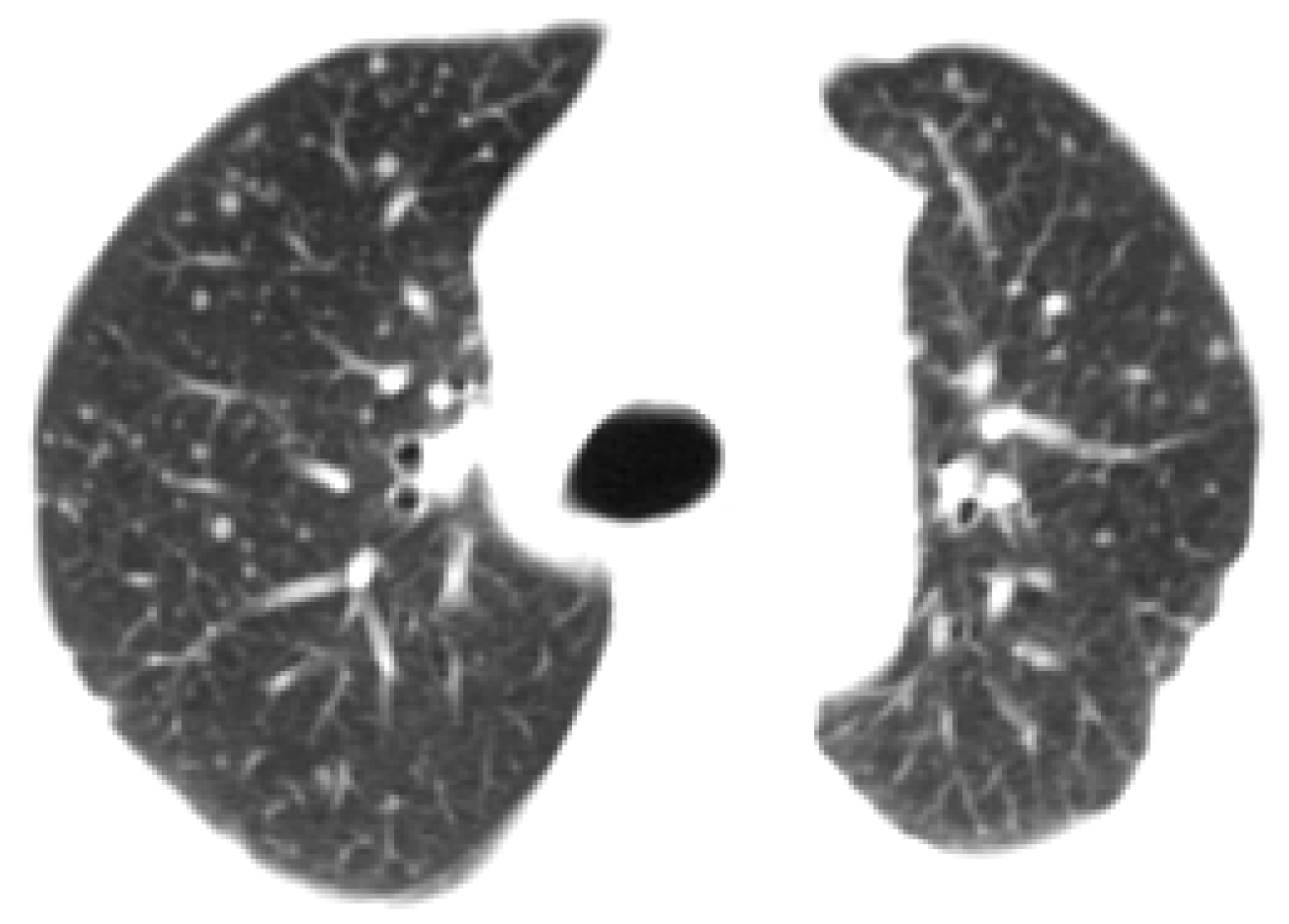
This step applies SVD to proceed with the decomposition and reconstruction of the lung images. Given an input lung image, IMG-A (see Figure 12; the pixel size is 512 × 512), the SVD method can decompose IMG-A as U × D × VT, where U and V are both a square matrix (512 × 512) and D is a singular diagonal matrix. The values of the diagonal cell in the D matrix are singular values of IMG-A. Figure 13 demonstrates the partial singular values for IMG-A. If more values are located in the upper left side, more important characteristics for IMG-A are generated. After the singular values are generated, we can reconstruct IMG-A with these values. More singular values are used for reconstruct, as a more distinct image is produced. Figure 14 demonstrates the reconstructed images with various singular values (10, 20, 30, and all).
Algorithm 2: Removing irrelevant background areas
Input: image I (size of I is width × height)
begin
  for i ⃪ 1 to width do
   for j ⃪ 1 to height
    if I ( i , j ) < 1
      I ( i , j ) = 1
    else if I ( i , j ) = 1 and j = j j + 9 I ( i , j ) < 10
     continue;
    else
    break;
    end
   end
  end
for i ⃪ 1 to width do
   for jheight to 1
    if I ( i , j ) < 1
      I ( i , j ) = 1
    else if I ( i , j ) = 1 and j = j j 9 I ( i , j ) < 10
     continue;
   else
    break;
    end
   end
  end
for j ⃪ 1 to height do
   for i ⃪ 1 to width do
    if I ( i , j ) < 1
      I ( i , j ) = 1
    else if I ( i , j ) = 1 and i = i i + 9 I ( i , j ) < 10
     continue;
    else
    break;
    end
   end
  end
for j ⃪ 1 to height do
   for iwidth to 1 do
    if I ( i , j ) < 1
      I ( i , j ) = 1
    else if I ( i , j ) = 1 and i = i i 9 I ( i , j ) < 10
     continue;
    else
    break;
    end
   end
  end
end
Output: image I
Algorithm 3: Outlining the lung areas with a box field
Input: image I (size of I is width × height)
begin
  x = 0, y = 0, W = 0, H = 0
  for i ⃪ 1 to width do
   for j ⃪ 1 to height
    if I ( i , j ) < 0.8
     x = i break
    end
   end
   if x 0
    break
   end
  end
  for iwidth to 1 do
   for j ⃪ 1 to height
    if I ( i , j ) < 0.8
     W = i break
    end
   end
   if W 0
    break
   end
  end
for j ⃪ 1 to height do
   for i ⃪ 1 to width do
    if I ( i , j ) < 0.8
     y = j break
    end
   end
   if y 0
    break
   end
  end
for jheight to 1 do
   for i ⃪ 1 to width do
    if I ( i , j ) < 0.8
     H = j break
    end
   end
   if H 0
    break
   end
  end
end
Output: image I crop from I ( x , y ) , width is W-x, and height is H-y
Step 4: Generating the Coefficient by DWPT
In this step, the discrete wavelet packet transform (DWPT) algorithm is applied to extract features (coefficients) from the lung images. Two sub-processes are involved:

3.3.4. The DWPT Decomposition Process

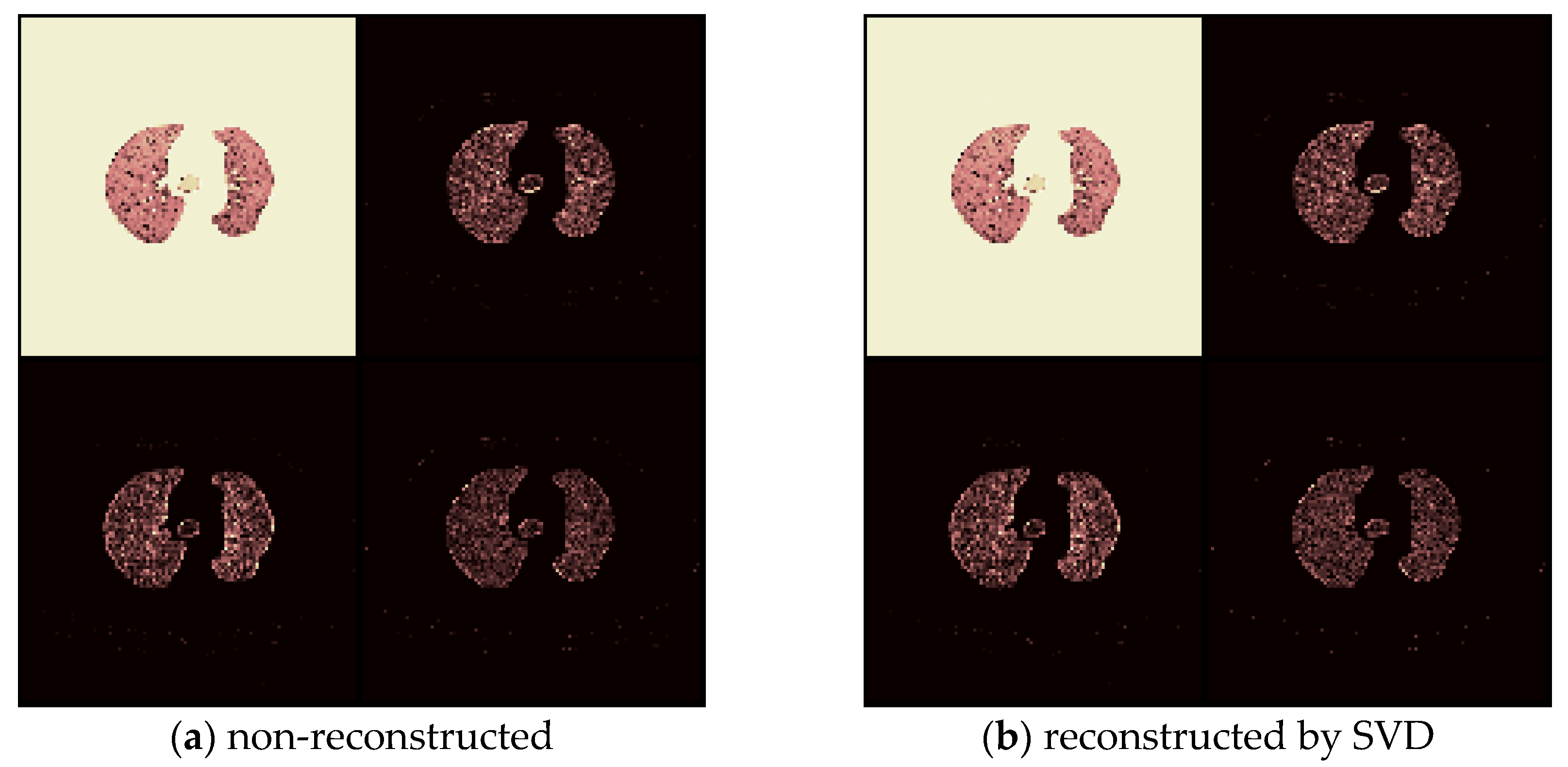
In this step, we use the DWPT algorithm to process the lung images and a multi-resolution pyramidal structure is applied with a depth m = 1 and 2. The four coefficients of DWPT (one approximate and three detailed coefficients) are produced for each image when m = 1 (Figure 15 illustrates lung images with four various DWPT coefficients for two types of images: non-reconstructed and reconstructed by SVD). There are 16 coefficients of DWPT (one approximate and 15 detailed coefficients) produced for each of the image regions when m = 2 (Figure 16 illustrates the lung images with 16 various DWPT coefficients for two types of images: non-reconstructed and reconstructed by SVD). Therefore, the amount of the DWPT coefficients is 16.

3.3.5. Wavelet Packet Entropy

“Entropy” is a popular approach that is applied to many research areas, such as image processing and signal processing. In DWPT coefficients, the wavelet packet norm entropy value can be generated by the following equation
Norm   entropy = 1 N i , j = 1 N | t ( i , j ) | p
where p is the power, whose numeric range is 1 ≤ p < 2, N is the size of the lung images, and t(i, j) is a transformed value in (i, j) for any sub-band (one of L-Li, L-Hi, H-Li, or H-Hi) of size N × N [28]. In this paper, we assign ‘1’ to p to produce wavelet packet norm entropy values.
Step 5: Computing the Feature Values and Reducing Attributes
This step computes the feature values of the wavelet packet for image datasets. Using Avei’s (2008) method, statistical values are used as inputs for the adaptive-network-based fuzzy inference system (ANFIS) [18]. This paper also applies these statistical feature values of wavelet packets to generate the following features: mean, median, mode, maximum, minimum, range, standard deviation, and the absolute values of the median and mean. In this step, we employ “reduct sets” to select the features of the wavelet packet. Reduct sets denote a subset of features that preserves the completely discernible information from its original information system [14].
Take Table 1 as an example. There are six reducts, size = 1 (size of reduct), Pos.Reg. = 1 (reduct depends totally on the set and 0 Pos.Reg. 1), and SC = 1 (the stability coefficient for the reduct and 0 stability 1). Based on Table 1, there are six features that can be employed as the inputs for the classification method: the range value, mean value, minimum value, maximum value, standard deviation, and mean absolute value.
Step 6: Classifying the Lung Image Dataset
In this step, we apply the intelligent classifier, the rough sets theory (LEM2 algorithm [22]), to classify eight lung image datasets (see Figure 2). The decision attributes of the LIDC image dataset include three classes: nodule, non-nodule and inflammation, while the RTH dataset contains two classes: nodule and non-nodule. The feature values of the DWPT coefficient are employed as conditional attributes. Using the rough sets algorithm, understandable rules for classifying lung images are generated, and system accuracy is improved for model verification.

4. Experimental Results and Discussions

In this paper, we employed the chest CT image of LIDC and RTH datasets to implement experiments for model evaluation. The image datasets both contained 100 chest CT images (with picture resolutions of 512 × 512). To evaluate the proposed system carefully, we conducted 10 sampling experiments with each image dataset to determine the method’s performance. Every experiment employed 40 images as an input dataset, randomly selected from the CT image dataset, and the ratio of training: testing was 3:1 (30 images were used for training, and 10 images were used for testing). The average and standard deviation of the classification accuracy for the 10 experiments are used as the performance indicators.
To verify the proposed system, we adopted many comparison methods in different processes. In image processing, the region-growing method (RGM) [25] (the processes of the RGM are illustrated in Figure A1 of the Appendix A) was used as the comparison method within the proposed method (the three-stage automated segmentation method, TSASM). In feature extraction, the DWPT method was used as a comparison method with the DWPT-SVD method. In the classification process, we employed four advanced methods, applied recently to analyze medical CT images, as comparison models: Trees.J48 [29], Naïve Bayes [30], Multilayer Perception [31], and Sequential Minimal Optimization (SMO) [32].
After the experiments were completed, many parameters were produced. For the processes of SVD reconstruction, the r values of each image are different, ranging from 255 to 478 for the two image datasets and, for the decomposition process, the number of the DWPT coefficients is 16. The experimental results (classification accuracy) for the proposed system and different comparison methods are shown from Table 2, Table 3, Table 4 and Table 5. Based on the performance data, we have discovered four findings as follows.
Firstly, from the performance data (Table 2 and Table 3), it is clear that the proposed system performs best in classification accuracy among the five listed methods (the proposed system: 99.41% for LIDC and 99.80% for RTH; Trees.J48: 87.42% for LIDC and 87.00% for RTH; Naïve Bayes: 83.18% for LIDC and 62.90% for RTH; Multilayer Perception: 84.48% for LIDC and 89.50% for RTH; SMO: 81.13% for LIDC and 71.40% for RTH). The standard deviation of classification accuracy for the proposed system (proposed system: 0.018 for LIDC and 0.037 for RTH) is much smaller than that of the comparison methods (Trees.J48: 9.68 for LIDC and 10.78 for RTH; Naïve Bayes: 10.51 for LIDC and 13.73 for RTH; Multilayer Perception: 11.16 for LIDC and 9.36 for RTH; SMO: 10.91 for LIDC and 13.41 for RTH). The proposed system performs perfectly and robustly in classification accuracy.
Secondly, the performance data (Table 2 and Table 3) also shows that the proposed image segmentation method (TSASM) improved the classification accuracy of the five listed classification methods. The accuracy for all methods is slightly better using TSASM than using RGM. For the LIDC dataset, the improvement of accuracy ranges from 1.61% to 8.02% (Rough set theory: 1.61%; Trees.J48: 8.02%; Naïve Bayes: 3.08%; Multilayer Perception: 4.68%; SMO: 3.73%). However, for the RTH dataset, the improvement is not as significant as that of the LIDC dataset, ranging from −4.5% to 5.5% (Rough set theory: 1.29%; Trees.J48:5.5%; Naïve Bayes: −4.5%; Multilayer Perception: 0.5.0 %; SMO: 0.40%). Based on the evidence, we argue that medical images’ quality and classification method both influence classification accuracy.
Thirdly, based on Table 4 and Table 5, the different signal transformation methods (DWPT and DWPT-SVD) lead to no significant improvements in classification accuracy (from 0.22% to 1.08% for the LIDC; from −0.20% to 2.20% for the RTH). Although the improvement is not high, this method contributed slightly to the improvement of diagnostic accuracy. For diseases with a high mortality rate, this level of improvement is also of importance.
Lastly, as seen in Table 2, Table 3, Table 4 and Table 5, the difference in the classification accuracy between the RTH and the RIDC for the proposed system is very small (The difference is “−0.61 %”) and insignificant statistically. The reason why the accuracy for the RTH is smaller than that of the LIDC is the difference in image quality between them (e.g., the radiologist’s experience in judging nodules, patient’s cooperation during CT image scanning, and equipment status issues for the CT scanner).
Although the proposed system has excellent classification accuracy in analyzing the chest CT images, more performance comparisons with similarly advanced methods in the related literature are required. Messay et al.’s computer-aided detection (CAD) system is able to correctly identify 80.4% of nodules (115/143) using 40 selected features of the LIDC datasets [24]. Li et al.’s computer-aided diagnosis (CAD) system can achieve an average pancreatic cancer identification accuracy of 96.47% from PET/CT data (from General Hospital of Shenyang Military Area Command) [31]. The sensitivity of nodule candidate detection in the advanced system developed by Xie et al. (2019), based on a 2D convolutional neural network (CNN), was 86.42% [33]. We can see that the identification accuracy for disease diagnosis with CT images has improved rapidly. Compared with Messay et al.’s (2010) system [24], our proposed system performs (99.41% for the LIDC and 98.80% for the RTH) outstandingly. Our system is more reasonable compared to Li et al.’s system (96.47%) [31]. We argue that the great improvement in identification accuracy for computer-aided system of disease diagnosis can be explained in three ways: (1) the knowledge progress of medical image specialists, (2) the improvement of image quality by next-generation scanners, and (3) the advances in image analysis algorithms by researchers.

5. Conclusions

According to the results reported in Table 2 to Table 5, the proposed system clearly performs best in classification accuracy among the five listed classifiers. Moreover, the standard deviation in classification accuracy for the proposed system is smaller than the comparison methods. This shows that the proposed system performs perfectly and robustly in term of classification accuracy. In segmentation, we see that the proposed image segmentation method (TSASM) improved the classification accuracy of the listed five classification methods (shown in Table 2 and Table 3). Based on the results, we argue that the medical image quality and classification method both influence classification accuracy. In signal transformation methods (DWPT and DWPT-SVD), there were no significant improvements in classification accuracy (as shown in Table 4 and Table 5). However, this method has contributed slightly to the improvement in diagnostic accuracy. Due to this disease’s high mortality rate, this level of improvement is also of importance.
Although the proposed system can efficiently improve classification accuracy and be qualified as a clinical decision-support system for diagnosing lung disease to increase clinical quality and efficiency, the accuracy of the classification results from the proposed system was still verified by medical specialists. From the experimental data, it is concluded that the classification algorithm plays a key role in accuracy, and medical image quality also plays a supporting role.
We offer two suggestions for future work: (1) other human organ CT imaging databases can be used to test the proposed system and examine its classification accuracy, and (2) other classification methods (e.g., k-nearest neighbors, random forest) can be applied to the classification process of the proposed system to examine its performance improvement.

Author Contributions

Conceptualization, C.-H.C.; methodology, C.-H.C.; validation, T.-L.C.; formal analysis: H.-H.C.; resources, H.-H.C.; data curation, H.-H.C.; writing—original, draft preparation, T.-L.C.; writing—review and editing, C.-H.C. All authors have read and agreed to the published version of the manuscript.

Funding

This research received no external funding

Acknowledgments

We would like to thank the editors and the two anonymous reviewers for their suggestions and help in improving this manuscript. We are also immensely grateful to the master’s student, Chaun-Yi Lin, for helping with the experiments in the earlier version of this manuscript.

Conflicts of Interest

The authors state that there are no conflicts of interest associated with this publication and there has been no significant financial support for this work that could have influenced its outcome.

Appendix A

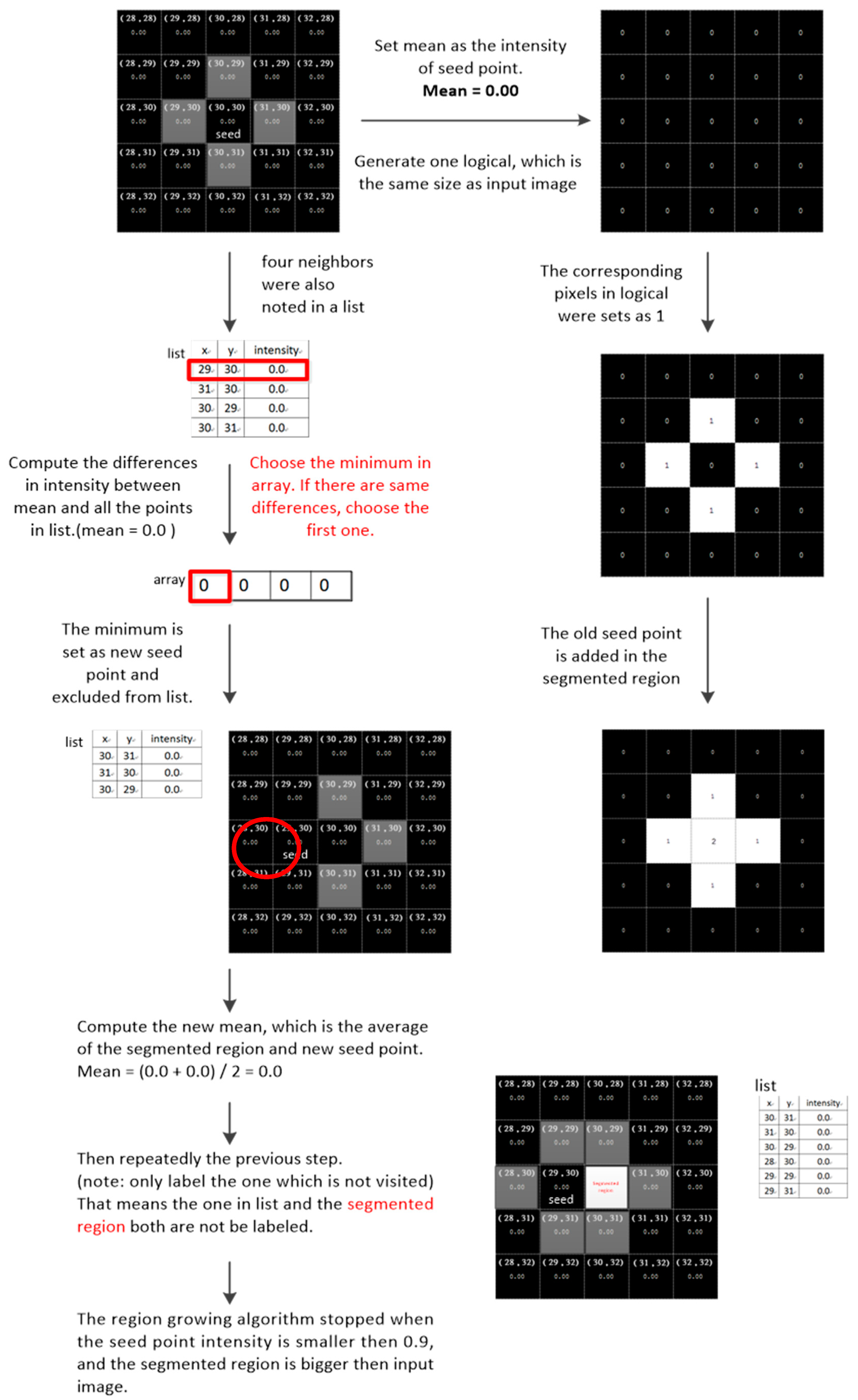
Figure A1. Region growing method.
Symmetry 12 00386 g0a1

References

  1. Sousa, J.R.; Silva, A.C.; De Paiva, A.C.; Nunes, R.A. Methodology for automatic detection of lung nodules in computerized tomography images. Comput. Methods Programs Biomed. 2010, 98, 1–14. [Google Scholar] [CrossRef] [PubMed]
  2. Souto, M.; Correa, J.; Tahoces, P.G.; Tucker, D.; Malagari, K.S.; Vidal, J.J.; Fraser, R.G. Enhancement of Chest Images by Automatic Adaptive Spatial Filtering. J. Digit. Imaging 1992, 4, 1–7. [Google Scholar] [CrossRef]
  3. Correa, J.; Souto, M.; Tahoces, P.G.; Malagari, K.; Tucker, D.; Larkin, J.; Kuhlman, J.; Barnes, G.T.; Zerhouni, E.; Fraser, R.G.; et al. Digital chest radiography: A comparison between unprocessed and processed images in the detection of solitary pulmonary nodules. Radiology 1995, 195, 253–258. [Google Scholar] [CrossRef] [PubMed]
  4. Helen, H.; Jeongjin, L.; Yeny, Y. Automatic lung nodule matching on sequential CT images. Comput. Biol. Med. 2008, 38, 623–634. [Google Scholar]
  5. Armato, S.G.; McLennan, G.; McNitt-Gray, M.F.; Meyer, C.R.; Yankelevitz, D.; Aberle, D.R.; Clarke, L.P. Lung image database consortium developing a resource for the medical imaging research community. Radiology 2004, 232, 739–748. [Google Scholar] [CrossRef] [PubMed]
  6. Lee, S.L.A.; Kouzani, A.Z.; Hu, E.J. Random forest based lung nodule classification aided by clustering. Comput. Med. Imaging Graph. 2010, 34, 535–542. [Google Scholar] [CrossRef]
  7. Mullaly, W.; Betke, M.; Hong, H.; Wang, J.; Mann, K.; Ko, J.P. Multi-criterion 3D segmentation and registration of pulmonary nodules on CT: A preliminary investigation. In Proceedings of the International Conference on Diagnostic Imaging and Analysis (ICDIA 2002), Shanghai, China, 18–20 August 2002; pp. 176–181. [Google Scholar]
  8. Dehmeshki, J.; Ye, X.; Lin, X.Y.; Valdivieso, M.; Amin, H. Automated detection of lung nodules in CT images using shape-based genetic algorithm. Comput. Med. Imaging Graph. 2007, 31, 408–417. [Google Scholar] [CrossRef]
  9. Yeny, Y.; Helen, H. Correction of segmented lung boundary for inclusion of pleural nodules and pulmonary vessels in chest CT images. Comput. Biol. Med. 2008, 38, 845–857. [Google Scholar]
  10. Mallat, S. A Wavelet Tour of Signal Processing; Academic Press: New York, NY, USA, 1999. [Google Scholar]
  11. Avci, E. An expert system based on Wavelet Neural Network-Adaptive Norm Entropy for scale invariant texture classification. Expert Syst. Appl. 2007, 32, 919–926. [Google Scholar] [CrossRef]
  12. Vozalis, M.G.; Margaritis, K.G. Using SVD and demographic data for the enhancement of generalized Collaborative Filtering. Inf. Sci. 2007, 177, 3017–3037. [Google Scholar] [CrossRef]
  13. Pawlak, Z. Rough sets. Int. J. Comput. Inf. Sci. 1982, 11, 341–356. [Google Scholar] [CrossRef]
  14. Pawlak, Z. Rough Sets: Theoretical Aspects of Reasoning about Data; Kluwer Academic Publisher: Boston, MA, USA, 1991. [Google Scholar]
  15. Pawlak, Z.; Skowron, A. Rudiments of rough sets. Inf. Sci. 2007, 177, 3–27. [Google Scholar] [CrossRef]
  16. Jothi, G.; Hannah Inbarani, H. Hybrid Tolerance Rough Set–Firefly based supervised feature selection for MRI brain tumor image classification. Appl. Soft Comput. 2016, 46, 639–651. [Google Scholar]
  17. Chung, K.L.; Yang, W.N.; Huang, Y.H.; Wu, S.T.; Hsu, Y.C. On SVD-based watermarking algorithm. Appl. Math. Comput. 2007, 188, 54–57. [Google Scholar] [CrossRef]
  18. Avci, E. Comparison of wavelet families for texture classification by using wavelet packet entropy adaptive network based fuzzy inference system. Appl. Soft Comput. 2008, 8, 225–231. [Google Scholar] [CrossRef]
  19. Avci, E.; Turkoglu, I.; Poyraz, M. A new approach based on scalogram for automatic target recognition with X-band Doppler radar. Asian J. Inf. Technol. 2005, 4, 133–140. [Google Scholar]
  20. Avci, E.; Turkoglu, I.; Poyraz, M. Intelligent target recognition based on wavelet packet neural network. Expert Syst. Appl. 2005, 29, 175–182. [Google Scholar] [CrossRef]
  21. Mallat, S.; Zhong, S. Characterization of signals from multiscale edges. IEEE Trans. Pattern Anal. Mach. Intell. 1992, 14, 710–732. [Google Scholar] [CrossRef] [Green Version]
  22. Huang, K.; Aviyente, S. Information-theoretic wavelet packet subband selection for texture classification. Signal Process. 2006, 86, 1410–1420. [Google Scholar] [CrossRef]
  23. Muneeswaran, K.; Ganesan, L.; Arumugam, S.; Soundar, K.R. Texture classification with combined rotation and scale invariant wavelet features. Pattern Recognit. 2005, 38, 1495–1506. [Google Scholar] [CrossRef]
  24. Messay, T.; Hardie, R.C.; Rogers, S.K. A new computationally efficient CAD system for pulmonary nodule detection in CT imagery. Med. Image Anal. 2010, 14, 390–406. [Google Scholar] [CrossRef] [PubMed]
  25. Gonzalez, R.C.; Woods, R.E. Digital Image Processing, 2nd ed.; Prentice-Hall: Englewood Cliffs, NJ, USA, 2002. [Google Scholar]
  26. Kroon, D.-J. Region Growing, MATLAB Central File Exchange. Available online: https://www.mathworks.com/matlabcentral/fileexchange/19084-region-growing (accessed on 25 February 2020).
  27. Grzymala-Busse, J.W. A new version of the rule induction system LERS. Fundam. Inform. 1997, 31, 27–39. [Google Scholar] [CrossRef]
  28. Arivazhagan, S.; Ganesan, L. Texture classification using wavelet transform. Pattern Recognit. Lett. 2003, 24, 1513–1521. [Google Scholar] [CrossRef]
  29. Witten, I.H.; Frank, E.; Hall, M.A.; Christopher, J.P. Data Mining: Practical Machine Learning Tools and Techniques, 4th ed.; Elsevier: Amsterdam, The Netherlands, 2017; pp. 67–89. [Google Scholar]
  30. Klement, W.; Wilk, S.; Michalowski, W.; Farion, K.J.; Osmond, M.H.; Verter, V. Predicting the need for CT imaging in children with minor head injury using an ensemble of Naive Bayes classifiers. Artif. Intell. Med. 2012, 54, 163–170. [Google Scholar] [CrossRef]
  31. Mohan, G.; Subashini, M.M. MRI based medical image analysis: Survey on brain tumor grade classification. Biomed. Signal Process. Control 2018, 39, 139–161. [Google Scholar] [CrossRef]
  32. Li, S.; Jiang, H.; Wang, Z.; Zhang, G.; Yao, Y.D. An effective computer aided diagnosis model for pancreas cancer on PET/CT images. Comput. Methods Programs Biomed. 2018, 165, 205–214. [Google Scholar] [CrossRef]
  33. Xie, H.T.; Yang, D.B.; Sun, N.N.; Chen, Z.N.; Zhang, Y.D. Automated pulmonary nodule detection in CT images using deep convolutional neural networks. Pattern Recognit. 2019, 85, 109–119. [Google Scholar] [CrossRef]
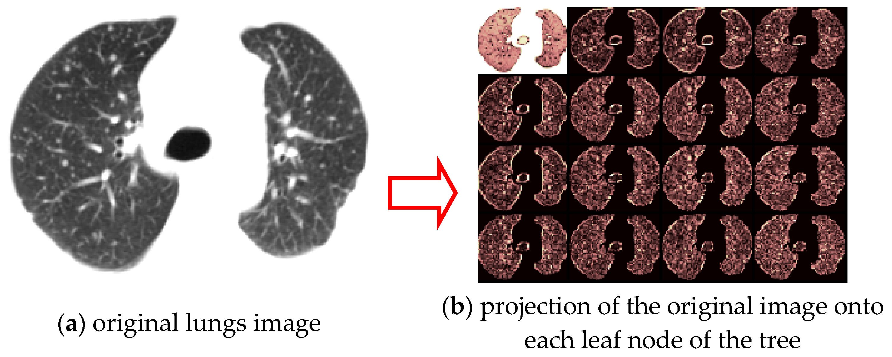
Figure 1. Decomposition of the 2-level DWPT.
Symmetry 12 00386 g001
Figure 2. The framework of the proposed system.
Symmetry 12 00386 g002
Figure 3. The original chest image.
Symmetry 12 00386 g003
Figure 4. The image adjusted by the contrast adjusting tool.
Symmetry 12 00386 g004
Figure 5. The histogram of Hounsfield units for the adjusted image.
Symmetry 12 00386 g005
Figure 6. The tuning process for expanding the display range.
Symmetry 12 00386 g006
Figure 7. The image after adjustment.
Symmetry 12 00386 g007
Figure 8. The image processing process using the proposed segmentation algorithms.
Symmetry 12 00386 g008
Figure 9. Process of segmenting a chest CT image.
Symmetry 12 00386 g009
Figure 10. Process for removing the irrelevant background areas.
Symmetry 12 00386 g010
Figure 11. Process of outlining the lung areas with a box field.
Symmetry 12 00386 g011
Figure 12. The image (IMG-A) for the singular value decomposition (SVD) image reconstruction process.
Symmetry 12 00386 g012
Figure 13. The singular values for the image (IMG-A).
Symmetry 12 00386 g013
Figure 14. The reconstructed images with 10, 20, 30, and all singular values for IMG-A.
Symmetry 12 00386 g014
Figure 15. Lung images with various discrete wavelet packets transform (DWPT) coefficients (m = 1, the amount of DWPT coefficient = 4).
Symmetry 12 00386 g015
Figure 16. Lung images based on various DWPT coefficients (m = 1, the amount of DWPT coefficient = 16).
Symmetry 12 00386 g016
Table 1. Reduct features of one dataset without SVD.
(1–6)SizePos.Reg.SCReducts
1111{range}
2111{mean}
3111{min}
4111{max}
5111{standard-deviation}
6111{mean-absolute-deviation }
Table 2. Classification accuracy for the proposed and comparison methods (LIDC dataset).
MethodProposedTreesNaïve BayesMultilayer PerceptionSMO
Region growing97.80% (0.038)79.40% (11.53)80.10% (12.35)79.80% (9.95)77.40% (10.21)
Proposed algorithm* 99.41% (0.018)87.42% (9.68)83.18% (10.51)84.48% (11.16)81.13% (10.91)
Note: * denoted the best accuracy among all combined methods, and each cell represents the average accuracy of 10 experiments with the standard deviation in parentheses.
Table 3. Classification accuracy for the proposed and comparison methods (RTH dataset).
MethodProposed TreesNaïve BayesMultilayer PerceptionSMO
Region growing97.51% (0.043)81.50% (12.58)67.40% (14.33)89.00% (10.68)71.00% (13.82)
Proposed algorithm* 98.80% (0.037)87.00%(10.78)62.90% (13.73)89.50% (9.36)71.40% (13.41)
Note: * denoted the best accuracy among all combined methods, and each cell represents the average accuracy of 10 experiments with the standard deviation in parentheses.
Table 4. Classification accuracy for DWPT-SVD and DWPT (LIDC dataset).
MethodRough SetsTrees.J48Naïve BayesMultilayer PerceptionSMO
Proposed system DWPT99.17% (0.026)86.90% (9.40)82.10% (11.83)84.70% (11.59)80.90% (10.55)
DWPT-SVD* 99.41% (0.018)87.42% (9.68)83.18% (10.51)84.48% (11.16)81.13% (10.91)
Note: * denoted the best accuracy among all combined methods, and each cell represents the average accuracy of 10 experiments with the standard deviation in parentheses.
Table 5. Classification accuracy for DWPT-SVD and DWPT (RTH dataset).
MethodRough SetsTrees.J48Naïve BayesMultilayer PerceptionSMO
Proposed systemDWPT98.66% (0.030)84.80% (11.05)62.90% (13.43)89.50% (9.47)71.60% (13.61)
DWPT-SVD* 98.80% (0.037)87.00% (10.78)62.90% (13.73)89.50% (9.36)71.40% (13.41)
Note: * denoted the best accuracy among all combined methods, and each cell represents the average accuracy of 10 experiments with the standard deviation in parentheses.