T-Spherical Fuzzy Einstein Hybrid Aggregation Operators and Their Applications in Multi-Attribute Decision Making Problems

Abstract

T-spherical fuzzy set is a recently developed model that copes with imprecise and uncertain events of real-life with the help of four functions having no restrictions. This article’s aim is to define some improved algebraic operations for T-SFSs known as Einstein sum, Einstein product and Einstein scalar multiplication based on Einstein t-norms and t-conorms. Then some geometric and averaging aggregation operators have been established based on defined Einstein operations. The validity of the defined aggregation operators has been investigated thoroughly. The multi-attribute decision-making method is described in the environment of T-SFSs and is supported by a comprehensive numerical example using the proposed Einstein aggregation tools. As consequences of the defined aggregation operators, the same concept of Einstein aggregation operators has been proposed for q-rung orthopair fuzzy sets, spherical fuzzy sets, Pythagorean fuzzy sets, picture fuzzy sets, and intuitionistic fuzzy sets. To signify the importance of proposed operators, a comparative analysis of proposed and existing studies is developed, and the results are analyzed numerically. The advantages of the proposed study are demonstrated numerically over the existing literature with the help of examples.

1. Introduction

To deal with imprecise and uncertain events has always been a challenging task as imprecision and vagueness lie in almost every field of science. To serve the goal, Zadeh [1] proposed the notion of a fuzzy set (FS) where he described the uncertainty of an object/event by a membership grade $m$ that has a value from the interval $\left[0,1\right]$. Atanassov [2] proposed the notion of the intuitionistic fuzzy set (IFS) based on two grades $m$ and $n$ representing the membership and non-membership degree of an object. Yager [3] proposed the idea of Pythagorean fuzzy set (PyFS) based on two grades $m$ and $n$ with the condition that the sum of squares of $m$ and $n$ must be less than or equal to 1. PyFS provides a considerably larger range for the values of $m$ and $n$ to be chosen but still, it has limited space. To obtain a space of membership and non-membership grades with no limitation, Yager [4] proposed the framework of q-rung orthopair fuzzy set (q-ROPFS) with the condition that the sum of the qth power of $m$ and $n$ must be less than or equal to 1, for a positive integer q. The constraints of these mentioned fuzzy frameworks are discussed in

Table 1. Fuzzy frameworks with their limitations).

Fuzzy Structures	Functions	Limitations on Functions
FS	$m$	$0\le m\le 1$
IFS	$\left(m, n\right)$	$0\le m+n\le 1$
PyFS	$\left(m, n\right)$	$0\le m^2+n^2\le 1$
q-ROPFS	$\left(m, n\right)$	$0\le m^q+n^q\le 1$, $q\in {\mathbb{Z}}^{+}$

.

All fuzzy models described in [1,2,3,4] either use one or two membership grades to model an event, but not all real-life events can always be modeled using these types of fuzzy frameworks. In 2013, Cuong [5] considered the situation of voting in which one may have four types of opinions including membership, abstinence, non-membership, and refusal degree. Cuong [5] used the four grades to model such events and developed the concept of the picture fuzzy set (PFS) with a restriction. The restriction on Cuong’s structure of PFS left no choice for decision makers to choose values of their consent for three functions $m, i$ and $n$ denoting membership, abstinence, and non-membership degree respectively. Realizing this problem, Mahmood et al. [6] developed the important concept of the spherical fuzzy set (SFS) and consequently the T-spherical fuzzy set (T-SFS). A T-SFS allows the decision makers to choose any value from closed unit interval regardless of any restriction. A description of the constraints of PFS, SFS and T-SFS is provided in

Table 2. Comparison of the restrictions of PFS, SFS and TSFS).

Fuzzy Structures	Functions	Limitations on Functions
PFS	$\left(m, i, n\right)$	$0\le m+i+n\le 1$
SFS	$\left(m,i, n\right)$	$0\le m^2+i^2+n^2\le 1$
T-SFS	$\left(m,i, n\right)$	$0\le m^t+i^t+n^t\le 1$, $t\in {\mathbb{Z}}^{+}$

.

A geometrical comparison among the ranges of PFSs, SFSs and T-SFSs is depicted in Figure 1 which is based on the constraints discussed in Table 2. All the numbers within and on the space of PFSs represent picture fuzzy numbers; all the numbers on and within the space of SFSs represent spherical fuzzy numbers; and all the numbers on and within space of T-SFSs represent T-spherical fuzzy numbers for $t=20$.

From Figure 1, it is easy to observe that T-SFS is much more generalized and diverse than PFS and SFS. The space for T-SFS increases with any increment in the value of $t$. This enables the experts to have much more values to assign to each membership, abstinence and non-membership grades.

Multi-attribute decision making (MADM) is one of the most discussed problems in FS theory due to its influence in engineering, economics and management sciences. The study of MADM started in 1970 [7] to use the concept of FS in a decision-making problem. Later, the concept of IFS and its aggregation tools have been greatly used in decision making problems. Xu [8] developed some aggregation operators (AOs) for IFSs and studied their applications in MADM. Klement and Mesiar [9] proposed some triangular norms. PyFSs also have been greatly utilized in MADM problems through some averaging and geometric aggregation tools developed by [10,11]. Cuong’s Structure of PFS has been utilized in MADM problems using the weighted geometric and averaging AOs of PFSs which have been developed by [12,13]. Mahmood at al. [6] developed some T-spherical fuzzy weighted geometric AOs and investigated their applications in MADM. Ullah et al. [14] solved a financial policy evaluation problem using interval-valued T-spherical fuzzy AOs. Ullah et al. [15] proposed some averaging AOs for T-SFSs and applied those operators to MADM problems. Liu et al. [16] introduced T-SF power Muirhead mean operators and utilized those operators in MADM problems. Garg et al. [17] dealt with MADM problems by introducing some T-spherical fuzzy interactive geometric AOs. For other notable work on the AOs of these fuzzy structures and their applications in MADM, one is referred to [18,19,20,21,22,23].

In the theory of aggregation, weighted geometric and averaging operators are the widely used operators and these are based on some t-norms and t-conorms. Literature survey witnessed some other types of t-norms and t-conorms, respectively—among them Einstein t-norm and t-conorms have got some serious attention. Based on Einstein t-conorms and t-norms, several aggregation tools have been proposed for various fuzzy algebraic structures. The Einstein weighted averaging (EWA) and Einstein weighted geometric (EWG) operators of IFSs and interval valued IFSs have been investigated in [24,25]. For PyFSs, EWA and Einstein interactive aggregation operators are developed by [26,27], respectively. For further interesting work on Einstein aggregation operators and their applications in MADM, one is referred to [28,29,30].

The continuous growth of interest has occurred in order to meet the requirements in needs of fertile applications of these inequalities. Such inequalities had been studied by many researchers who in turn used various techniques for the sake of exploring and offering these inequalities [31,32,33,34,35,36,37,38,39,40,41,42] and the references cited therein.

By analyzing the literature, no significant work can be found on EWA and EWG operators in the environment of PFSs, q-ROPFS, SFSs and T-SFSs. Keeping in mind the developments of Einstein aggregation operators, in this manuscript, some averaging, as well as geometric AOs, are produced based on Einstein operations for T-SFSs. Using the Einstein operations of T-SFSs, the same concepts are also defined for q-ROPFSs, PFSs, and SFSs as consequences of new proposed work. Furthermore, the generalization of new proposed work has also been discussed.

The remaining article is organized as section one provides a brief history of the fuzzy structure and theory of aggregation operators. Section 2 provides some initial concepts related to T-SFSs, SFSs, PFSs, q-ROPFSs, PyFSs and IFSs. In Section 3, we proposed the Einstein sum and Einstein product for T-SFSs. We also defined the Einstein sum and product for SFSs, q-ROPFS, and PFSs in a remark. Section 4 is based on the weighted averaging, ordered weighted averaging and hybrid averaging operators for T-SFSs based on Einstein sum; while Section 5 is based on the weighted geometric, ordered weighted geometric and hybrid geometric operators for T-SFSs based on Einstein product. In Section 6, the defined aggregation tools have used MADM. Section 7 provides the advantages of the proposed work. Further, with the help of some useful conditions, EWA and EWG operators are also defined for q-ROPFSs, SFSs and PFSs. A comparative analysis is also discussed with the help of examples. In Section 8, we summarized the article by pointing out some future study. The list of abbreviations adopted hereafter is given in

Table 3. Abbreviation Values.

Definition	Abbreviation
Fuzzy set	FS
Intuitionistic fuzzy set	IFS
Pythagorean fuzzy set	PyFS
q-rung orthopair fuzzy set	q-ROPFS
Picture fuzzy set	PFS
Spherical fuzzy set	SFS
T-spherical fuzzy set	T-SFS
Aggregation operator	AO
Einstein weighted averaging	EWA
Einstein weighted geometric	EWG
T-spherical fuzzy Einstein weighted averaging	T-SFEWA
T-spherical fuzzy Einstein ordered weighted averaging	T-SFEOWA
T-spherical fuzzy Einstein hybrid averaging	T-SFEHA
T-spherical fuzzy Einstein weighted geometric	T-SFEWG
T-spherical fuzzy Einstein ordered weighted geometric	T-SFEOWG
T-spherical fuzzy Einstein hybrid geometric	T-SFEHG
multi-attribute decision making	MADM

:

2. Preliminaries

Some basic notions of T-SFSs, q-ROPFSs, SFSs, PyFSs, PFSs and IFSs are provided in this section. Furthermore, the concepts of Einstein t-norm and t-conorm are also studied in the existing fuzzy environments.

Definition 1.

[6] A T-SFS on $X\ne \varphi$ is defined as

$$P=\left\{\left(x,m\left(x\right),i\left(x\right),n\left(x\right)\right)x\in X\right\}$$

where $m,i,n:X\to \left[0,1\right]$, a membership, abstinence and non-membership function respectively, with the condition $0\le m^t\left(x\right)+i^t\left(x\right)+n^t\left(x\right)\le 1 \forall x\in X \& t\in {\mathbb{Z}}^{+}$. Further, $\mathrm{r}\left(\mathrm{x}\right)=\sqrt[\mathrm{t}]{1-\left({\mathrm{m}}^{\mathrm{t}}\left(\mathrm{x}\right)+{\mathrm{i}}^{\mathrm{t}}\left(\mathrm{x}\right)+{\mathrm{n}}^{\mathrm{t}}\left(\mathrm{x}\right)\right)}$ is called the refusal degree of $\mathrm{x}$ in $\mathrm{P}$ and the triplet $\left(\mathrm{m},\mathrm{i},\mathrm{n}\right)$ is known as T-spherical fuzzy number (T-SFN).

Remark 1.

i. 

The above definition becomes valid to SFS for$t=2$

ii. 

The above definition becomes valid to PFS for$t=1$

iii. 

The above definition becomes valid to q-ROPFS for$i=0$

iv. 

The above definition becomes valid to PyFS for $t=2$ and $i=0$

v. 

The above definition becomes valid to IFS for $t=1$ and $i=0$

vi. 

The above definition becomes valid to FS for $t=1$, $i=0$ and $n=0$

Definition 2.

[6] Let $P=\left(m,i,n\right)$ be a T-SFN. Then, the score value is defined as $\mathrm{SC}\left(\mathrm{P}\right)={\mathrm{m}}^{\mathrm{t}}\left(\mathrm{x}\right)-{\mathrm{n}}^{\mathrm{t}}\left(\mathrm{x}\right)$ and accuracy is defined as $AC\left(P\right)=m^t\left(x\right)+i^t\left(x\right)+n^t\left(x\right)$.

For $P_1=\left(m_1,i_1,n_1\right)$ and $P_2=\left(m_2,i_2,n_2\right)$ be any two T-SFNs then $P_1$ is superior than $P_2$ if $SC\left(P_1\right)>SC\left(P_2\right)$. If $SC\left(P_1\right)=SC\left(P_2\right)$ then superiority is checked by accuracy. If $AC\left(P_1\right)>AC\left(P_2\right)$ then $P_1$ is superior than $P_2$. If again $AC\left(P_1\right)=AC\left(P_2\right)$ then $P_1$ and $P_2$ are considered as similar.

Definition 3.

[9] Einstein operations consist of Einstein product which is example of t-norm and Einstein sum which is an example of t-conorm. Einstein Product and Einstein sum are defined as:

i. 

$m_1\otimes m_2=\frac{m_1{m}_2}{1+\left(1-m_1\right)\left(1-m_2\right)}$

ii. 

$m_1\oplus m_2=\frac{m_1+m_2}{1+m_1{m}_2}$

3. Einstein Operations for T-SFS

In this section, some Einstein operators for T-SFS are proposed with the help of Einstein sum and Einstein product. Some special cases of proposed operators are also discussed in the remark.

Definition 4.

Let $P_1=\left(m_1, i_1, n_1\right)$ and $P_2=\left(m_2, i_2, n_2\right)$ be two T-SFNs. Then their Einstein operations are defined as follows:

i. 

$P_1\le P_2 \Rightarrow m_1\le m_2, i_1\le i_2, n_1\ge n_2$

ii. 

$P_1\otimes P_2=\left(\sqrt[t]{\frac{m_1^t{m}_2^t}{1+\left(1-m_1^t\right)\left(1-m_2^t\right)}}, \sqrt[t]{\frac{i_1^t{i}_2^t}{1+\left(1-i_1^t\right)\left(1-i_2^t\right)}}, \sqrt[t]{\frac{n_1^t+n_2^t}{1+n_1^t{n}_2^t}}\right)$

iii. 

$P_1\oplus P_2=\left(\sqrt[t]{\frac{m_1^t+m_2^t}{1+\left(m_1^t+i_1^t\right)\left(m_2^t+i_2^t\right)-i_1^t{i}_2^t}}, \sqrt[t]{\frac{i_1^t{i}_2^t}{1+\left(1-i_1^t\right)\left(1-i_2^t\right)}}, \sqrt[t]{\frac{n_1^t{n}_2^t}{1+\left(1-n_1^t\right)\left(1-n_2^t\right)}} \right)$

iv. 

$\lambda P_1=\left(\sqrt[t]{\frac{{\left(1+m_1^t\right)}^{\lambda }-{\left(1-m_1^t\right)}^{\lambda }}{{\left(1+m_1^t\right)}^{\lambda }+{\left(1-m_1^t\right)}^{\lambda }}}, \sqrt[t]{\frac{{\left(2i_1^t\right)}^{\lambda }}{{\left(2-i_1^t\right)}^{\lambda }+{\left(i_1^t\right)}^{\lambda }}}, \sqrt[t]{\frac{{\left(2n_1^t\right)}^{\lambda }}{{\left(2-n_1^t\right)}^{\lambda }+{\left(n_1^t\right)}^{\lambda }}}\right), \lambda >0$

v. 

$P_1^{\lambda }=\left(\sqrt[t]{\frac{2{\left(m_1^t\right)}^{\lambda }}{{\left(2+m_1^t\right)}^{\lambda }+{\left(m_1^t\right)}^{\lambda }}}, \sqrt[t]{\frac{{\left(2i_1^t\right)}^{\lambda }}{{\left(2-i_1^t\right)}^{\lambda }+{\left(i_1^t\right)}^{\lambda }}},\sqrt[t]{\frac{{\left(1+n_1^t\right)}^{\lambda }-{\left(1-n_1^t\right)}^{\lambda }}{{\left(1+n_1^t\right)}^{\lambda }+{\left(1-n_1^t\right)}^{\lambda }}}\right), \lambda >0$

Remark 2.

i. 

For $t=2$, above operations become valid for SFSs

ii. 

For $t=1$, above operations become valid for PFSs

iii. 

For $i=0$, above operations become valid for q-ROPFSs

iv. 

For $t=2$ and $i=0$, above operations become valid for PyFSs

v. 

For $t=1$ and $i=0$, above operations become valid for IFSs

4. T-Spherical Fuzzy Einstein Hybrid Averaging Operators

In this section, by using Einstein operations, T-SF Einstein weighted averaging (T-SFEWA) operators, T-SF Einstein ordered weighted averaging (T-SFEOWA) operators, T-SF Einstein hybrid averaging (T-SFEHA) operators are defined and some of their properties are also discussed.

Definition 5.

For any collection, $P_j=\left(m_j,i_j,n_j\right)$ for all $j=1,2,3,\dots ,k$ of T-SFS,

$T-SFEW{A}_w\left(P_1,P_2,\dots ,P_k\right)={\oplus }_{j=1}^k{w}_j{P}_j$

$$=\left(\begin{array}{c}\sqrt[t]{\frac{{\prod }_{j=1}^k{\left(1+m_j^t\right)}^{w_j}-{\prod }_{j=1}^k{\left(1-m_j^t\right)}^{w_j}}{{\prod }_{j=1}^k{\left(1+m_j^t\right)}^{w_j}+{\prod }_{j=1}^k{\left(1-m_j^t\right)}^{w_j}}}, \sqrt[t]{\frac{2{\prod }_{j=1}^k{(i_j^t)}^{w_j}}{{\prod }_{j=1}^k{\left(2-i_j^t\right)}^{w_j}+{\prod }_{j=1}^k{\left(i_j^t\right)}^{w_j}}},\\ \sqrt[t]{\frac{2{\prod }_{j=1}^k{(n_j^t)}^{w_j}}{{\prod }_{j=1}^k{\left(2-n_j^t\right)}^{w_j}+{\prod }_{j=1}^k{\left(n_j^t\right)}^{w_j}}}\end{array}\right)$$

(1)

is called $\mathrm{T}-\mathrm{SFEWA}$ operator with weighting vector $\mathrm{w}={\left({\mathrm{w}}_1,{ \mathrm{w}}_2,\dots ,{\mathrm{w}}_{\mathrm{k}}\right)}^{\mathrm{T}}$ of ${\mathrm{P}}_{\mathrm{j}}$, where ${\mathrm{w}}_{\mathrm{j}}\in \left(0,1\right]$ and ${\sum }_{\mathrm{j}=1}^{\mathrm{k}}{\mathrm{w}}_{\mathrm{j}}=1$.

Theorem 1.

(Idempotency) If $P_j=P_0$ for all $j$, then $T-SFEW{A}_w\left(P_1,P_2,\dots ,P_k\right)=P_0$.

Proof. 

Since $P_j=P_0=\left(m_0,i_0,n_0\right)$ for all $j=1,2,3,\dots ,k$ and ${\sum }_{j=1}^k{w}_j=1$. Then

$$T-SFEW{A}_w\left(P_1,P_2,\dots ,P_k\right)=$$

$$\begin{array}{c}\left(\sqrt[t]{\frac{{\prod }_{j=1}^k{\left(1+m_0^t\right)}^{w_j}-{\prod }_{j=1}^k{\left(1-m_0^t\right)}^{w_j}}{{\prod }_{j=1}^k{\left(1+m_0^t\right)}^{w_j}+{\prod }_{j=1}^k{\left(1-m_0^t\right)}^{w_j}}}, \sqrt[t]{\frac{2{\prod }_{j=1}^k{(i_0^t)}^{w_j}}{{\prod }_{j=1}^k{\left(2-i_0^t\right)}^{w_j}+{\prod }_{j=1}^k{\left(i_0^t\right)}^{w_j}}}, \sqrt[t]{\frac{2{\prod }_{j=1}^k{(n_0^t)}^{w_j}}{{\prod }_{j=1}^k{\left(2-n_0^t\right)}^{w_j}+{\prod }_{j=1}^k{\left(n_0^t\right)}^{w_j}}}\right)\hfill \\ =\left(\sqrt[t]{\frac{{\left(1+m_0^t\right)}^{{\sum }_{j=1}^k{w}_j}-{\left(1-m_0^t\right)}^{{\sum }_{j=1}^k{w}_j}}{{\left(1+m_0^t\right)}^{{\sum }_{j=1}^k{w}_j}+{\left(1-m_0^t\right)}^{{\sum }_{j=1}^k{w}_j}}}, \sqrt[t]{\frac{2{(i_0^t)}^{{\sum }_{j=1}^k{w}_j}}{{\left(2-i_0^t\right)}^{{\sum }_{j=1}^k{w}_j}+{\left(i_0^t\right)}^{{\sum }_{j=1}^k{w}_j}}}, \sqrt[t]{\frac{2{(n_0^t)}^{{\sum }_{j=1}^k{w}_j}}{{\left(2-n_0^t\right)}^{{\sum }_{j=1}^k{w}_j}+{\left(n_0^t\right)}^{{\sum }_{j=1}^k{w}_j}}}\right)\hfill \\ =\left(m_0,i_0,n_0\right)=P_0.\hfill \end{array}$$

 □

Theorem 2.

(Boundedness) For a collection of T-SFNs $P_j \mathrm{for} \mathrm{all} j=1,2,3,\dots ,k$ and $P^L=\underset{j}{\min }{P}_j$, and $P^U=\underset{j}{\max }{P}_j$. Then

$$P^L\le T-SFEW{A}_w\left(P_1,P_2,\dots ,P_k\right)\le P^U$$

Proof. 

As $P^L=\underset{j}{\min }{P}_j=\left(\min m_j, \min i_j, \max n_j\right)$ and $P^U=\underset{j}{\max }{P}_j=\left(\max m_j, \max i_j, \min n_j\right)$. Then

$$\min m_j\le m_j\le \max m_j$$

$$\min m_j^t\le m_j^t\le \max m_j^t$$

$$1+\min m_j^t\le 1+m_j^t\le 1+\max m_j^t$$

$${\left(1+\min m_j^t\right)}^{w_j}\le {\displaystyle \prod }_{j=1}^k{\left(1+m_j^t\right)}^{w_j}\le {\left(1+\max m_j^t\right)}^{w_j}$$

$$\begin{gathered} \Rightarrow \sqrt[t]{\frac{{\left(1+\min m_j^t\right)}^{w_j}-{\left(1-\min m_j^t\right)}^{w_j}}{{\left(1+\min m_j^t\right)}^{w_j}+{\left(1-\min m_j^t\right)}^{w_j}}}\le \sqrt[t]{\frac{{\prod }_{j=1}^k{\left(1+m_j^t\right)}^{w_j}-{\prod }_{j=1}^k{\left(1-m_j^t\right)}^{w_j}}{{\prod }_{j=1}^k{\left(1+m_j^t\right)}^{w_j}+{\prod }_{j=1}^k{\left(1-m_j^t\right)}^{w_j}}} \\ \le \sqrt[t]{\frac{{\left(1+\max m_j^t\right)}^{w_j}-{\left(1-\max m_j^t\right)}^{w_j}}{{\left(1+\max m_j^t\right)}^{w_j}+{\left(1-\max m_j^t\right)}^{w_j}}} \end{gathered}$$

Now, $\min i_j\le i_j\le \max i_j$

$$\begin{gathered} \min i_j^t\le i_j^t\le \max i_j^t \\ 2\min {\left(i_j^t\right)}^{w_j}\le 2{\displaystyle \prod }_{j=1}^k{\left(i_j^t\right)}^{w_j}\le 2\max {\left(i_j^t\right)}^{w_j} \end{gathered}$$

$$(1)\Rightarrow \sqrt[t]{\frac{2\min {\left(i_j^t\right)}^{w_j}}{{\left(2-\min i_j^t\right)}^{w_j}+\min {\left(i_j^t\right)}^{w_j}}}\le \sqrt[t]{\frac{2{\prod }_{j=1}^k{(i_j^t)}^{w_j}}{{\prod }_{j=1}^k{\left(2-i_j^t\right)}^{w_j}+{\prod }_{j=1}^k{\left(i_j^t\right)}^{w_j}}}\le \sqrt[t]{\frac{2\max {\left(i_j^t\right)}^{w_j}}{{\left(2-\max i_j^t\right)}^{w_j}+\max {\left(i_j^t\right)}^{w_j}}}$$

Similarly, $\max n_j\ge n_j\ge \min n_j$

$$\begin{gathered} \max n_j^t\ge n_j^t\ge \min n_j^t \\ 2\max {\left(n_j^t\right)}^{w_j}\ge 2{\displaystyle \prod }_{j=1}^k{\left(n_j^t\right)}^{w_j}\ge 2\min {\left(n_j^t\right)}^{w_j} \\ \Rightarrow \sqrt[t]{\frac{2\max {\left(n_j^t\right)}^{w_j}}{{\left(2-\max n_j^t\right)}^{w_j}+\max {\left(n_j^t\right)}^{w_j}}}\ge \sqrt[t]{\frac{2{\prod }_{j=1}^k{(n_j^t)}^{w_j}}{{\prod }_{j=1}^k{\left(2-n_j^t\right)}^{w_j}+{\prod }_{j=1}^k{\left(n_j^t\right)}^{w_j}}} \\ \ge \sqrt[t]{\frac{2\min {\left(n_j^t\right)}^{w_j}}{{\left(2-\min n_j^t\right)}^{w_j}+\min {\left(n_j^t\right)}^{w_j}}} \\ \Rightarrow P^L\le T-SFEW{A}_w\left(P_1,P_2,\dots ,P_k\right)\le P^U \end{gathered}$$

 □

Theorem 3.

(Monotonicity) For any two T-SFNs $P_j=\left(m_j, i_j, n_j\right)$ and $P_j^{\prime }=\left(m_j^{\prime }, i_j^{\prime }, n_j^{\prime }\right)$ such that $P_j\le P_j^{\prime }$ for all $j=1,2,3,\dots ,k$. Then

$$T-SFEW{A}_w\left(P_1,P_2,\dots ,P_k\right)\le T-SFEW{A}_w\left(P_1,P_2,\dots ,P_k\right)$$

As,$m_j\le m_j^{\prime } \Rightarrow m_j^t\le {\left(m_j^{\prime }\right)}^t$

$$\begin{gathered} \Rightarrow 1+m_j^t\le 1+{\left(m_j^{\prime }\right)}^t \\ {\displaystyle \prod }_{j=1}^k{\left(1+m_j^t\right)}^{w_j}\le {\displaystyle \prod }_{j=1}^k{\left(1+{\left(m_j^{\prime }\right)}^t\right)}^{w_j} \\ \sqrt[t]{\frac{{\prod }_{j=1}^k{\left(1+m_j^t\right)}^{w_j}-{\prod }_{j=1}^k{\left(1-m_j^t\right)}^{w_j}}{{\prod }_{j=1}^k{\left(1+m_j^t\right)}^{w_j}+{\prod }_{j=1}^k{\left(1-m_j^t\right)}^{w_j}}}\le \sqrt[t]{\frac{{\prod }_{j=1}^k{\left(1+{\left(m_j^{\prime }\right)}^t\right)}^{w_j}-{\prod }_{j=1}^k{\left(1-{\left(m_j^{\prime }\right)}^t\right)}^{w_j}}{{\prod }_{j=1}^k{\left(1+{\left(m_j^{\prime }\right)}^t\right)}^{w_j}+{\prod }_{j=1}^k{\left(1-{\left(m_j^{\prime }\right)}^t\right)}^{w_j}}} \end{gathered}$$

As,$i_j\le i_j^{\prime } \Rightarrow i_j^t\le {\left(i_j^{\prime }\right)}^t$

$$\Rightarrow 2{\displaystyle \prod }_{j=1}^k{\left(i_j^t\right)}^{w_j}\le 2{\displaystyle \prod }_{j=1}^k{\left({\left(i_j^{\prime }\right)}^t\right)}^{w_j}$$

$$\sqrt[t]{\frac{2{\prod }_{j=1}^k{(i_j^t)}^{w_j}}{{\prod }_{j=1}^k{\left(2-i_j^t\right)}^{w_j}+{\prod }_{j=1}^k{\left(i_j^t\right)}^{w_j}}}\le \sqrt[t]{\frac{2{\prod }_{j=1}^k{\left({\left(i_j^{\prime }\right)}^t\right)}^{w_j}}{{\prod }_{j=1}^k{\left(2-{\left(i_j^{\prime }\right)}^t\right)}^{w_j}+{\prod }_{j=1}^k{\left({\left(i_j^{\prime }\right)}^t\right)}^{w_j}}}$$

Similarly,$n_j\ge n_j^{\prime } \Rightarrow n_j^t\ge {\left(n_j^{\prime }\right)}^t$

$$\begin{gathered} \Rightarrow 2{\displaystyle \prod }_{j=1}^k{\left(n_j^t\right)}^{w_j}\ge 2{\displaystyle \prod }_{j=1}^k{\left({\left(n_j^{\prime }\right)}^t\right)}^{w_j} \\ \sqrt[t]{\frac{2{\prod }_{j=1}^k{(n_j^t)}^{w_j}}{{\prod }_{j=1}^k{\left(2-n_j^t\right)}^{w_j}+{\prod }_{j=1}^k{\left(n_j^t\right)}^{w_j}}}\ge \sqrt[t]{\frac{2{\prod }_{j=1}^k{\left({\left(n_j^{\prime }\right)}^t\right)}^{w_j}}{{\prod }_{j=1}^k{\left(2-{\left(n_j^{\prime }\right)}^t\right)}^{w_j}+{\prod }_{j=1}^k{\left({\left(n_j^{\prime }\right)}^t\right)}^{w_j}}} \\ \Rightarrow T-SFEW{A}_w\left(P_1,P_2,\dots ,P_k\right)\le T-SFEW{A}_w\left(P_1,P_2,\dots ,P_k\right) \end{gathered}$$

Definition 6.

For any collection $P_j=\left(m_j,i_j,n_j\right) \mathrm{for} \mathrm{all} j=1,2,3,\dots ,k$ of T-SFS. Then

$$T-SFEOW{A}_{\omega }\left(P_1,P_2,\dots ,P_k\right)={\oplus }_{j=1}^k{\omega }_j{P}_{\sigma \left(j\right)}$$

$$=\left(\begin{array}{c}\sqrt[t]{\frac{{\prod }_{j=1}^k{\left(1+m_{\sigma \left(j\right)}^t\right)}^{{\omega }_j}-{\prod }_{j=1}^k{\left(1-m_{\sigma \left(j\right)}^t\right)}^{{\omega }_j}}{{\prod }_{j=1}^k{\left(1+m_{\sigma \left(j\right)}^t\right)}^{{\omega }_j}+{\prod }_{j=1}^k{\left(1-m_{\sigma \left(j\right)}^t\right)}^{{\omega }_j}}}, \sqrt[t]{\frac{2{\prod }_{j=1}^k{(i_{\sigma \left(j\right)}^t)}^{{\omega }_j}}{{\prod }_{j=1}^k{\left(2-i_{\sigma \left(j\right)}^t\right)}^{{\omega }_j}+{\prod }_{j=1}^k{\left(i_{\sigma \left(j\right)}^t\right)}^{{\omega }_j}}},\\ \sqrt[t]{\frac{2{\prod }_{j=1}^k{(n_{\sigma \left(j\right)}^t)}^{{\omega }_j}}{{\prod }_{j=1}^k{\left(2-n_{\sigma \left(j\right)}^t\right)}^{{\omega }_j}+{\prod }_{j=1}^k{\left(n_{\sigma \left(j\right)}^t\right)}^{{\omega }_j}}}\end{array}\right)$$

(2)

then $T-SFEOW{A}_{\omega }$ is called $T-SFEOWA$ operator with associated weight vector $\omega ={\left({\omega }_1, {\omega }_2,\dots ,{\omega }_k\right)}^T$ of $P_j$, where ${\omega }_j\in \left(0,1\right]$ and ${\sum }_{j=1}^k{\omega }_j=1$. $\sigma \left(j\right)$ is the permutation with respect to score value such that $SC\left(P_{\sigma \left(j-1\right)}\right)\ge SC\left(P_{\sigma \left(j\right)}\right)$.

In next theorems, idempotency, boundedness, and monotonicity properties are proved for the above operator.

Theorem 4.

If $P_j=P_0$ for all $j=1,2,3,\dots ,k$, then $T-SFEOW{A}_{\omega }\left(P_1,P_2,\dots ,P_k\right)=P_0$.

Proof. 

Since $P_j=P_0=\left(m_0,i_0,n_0\right)$ for all $j=1,2,3,\dots ,k$ and ${\sum }_{j=1}^k{\omega }_j=1$. Then

$$T-SFEOW{A}_{\omega }\left(P_1,P_2,\dots ,P_k\right)=$$

$$\begin{array}{c}\left(\sqrt[t]{\frac{{\prod }_{j=1}^k{\left(1+m_0^t\right)}^{{\omega }_j}-{\prod }_{j=1}^k{\left(1-m_0^t\right)}^{{\omega }_j}}{{\prod }_{j=1}^k{\left(1+m_0^t\right)}^{{\omega }_j}+{\prod }_{j=1}^k{\left(1-m_0^t\right)}^{{\omega }_j}}}, \sqrt[t]{\frac{2{\prod }_{j=1}^k{(i_0^t)}^{{\omega }_j}}{{\prod }_{j=1}^k{\left(2-i_0^t\right)}^{{\omega }_j}+{\prod }_{j=1}^k{\left(i_0^t\right)}^{{\omega }_j}}}, \sqrt[t]{\frac{2{\prod }_{j=1}^k{(n_0^t)}^{{\omega }_j}}{{\prod }_{j=1}^k{\left(2-n_0^t\right)}^{{\omega }_j}+{\prod }_{j=1}^k{\left(n_0^t\right)}^{{\omega }_j}}}\right)\hfill \\ =\left(\sqrt[t]{\frac{{\left(1+m_0^t\right)}^{{\sum }_{j=1}^k{\omega }_j}-{\left(1-m_0^t\right)}^{{\sum }_{j=1}^k{\omega }_j}}{{\left(1+m_0^t\right)}^{{\sum }_{j=1}^k{\omega }_j}+{\left(1-m_0^t\right)}^{{\sum }_{j=1}^k{\omega }_j}}}, \sqrt[t]{\frac{2{(i_0^t)}^{{\sum }_{j=1}^k{\omega }_j}}{{\left(2-i_0^t\right)}^{{\sum }_{j=1}^k{\omega }_j}+{\left(i_0^t\right)}^{{\sum }_{j=1}^k{\omega }_j}}}, \sqrt[t]{\frac{2{(n_0^t)}^{{\sum }_{j=1}^k{\omega }_j}}{{\left(2-n_0^t\right)}^{{\sum }_{j=1}^k{\omega }_j}+{\left(n_0^t\right)}^{{\sum }_{j=1}^k{\omega }_j}}}\right)\hfill \\ =\left(m_0,i_0,n_0\right)=P_0.\hfill \end{array}$$

 □

Theorem 5.

For a collection of T-SFNs $P_j$ for all $j=1,2,3,\dots ,k$ and $P^L=\underset{j}{\min }{P}_j$, and $P^U=\underset{j}{\max }{P}_j$. Then

$$P^L\le T-SFEOW{A}_{\omega }\left(P_1,P_2,\dots ,P_k\right)\le P^U$$

Proof. 

As $P^L=\underset{j}{\min }{P}_{\sigma \left(j\right)}=\left(\min m_{\sigma \left(j\right)}, \min i_{\sigma \left(j\right)}, \max n_{\sigma \left(j\right)}\right)$ and $P^U=\underset{j}{\max }{P}_{\sigma \left(j\right)}=\left(\max m_{\sigma \left(j\right)}, \max i_{\sigma \left(j\right)}, \min n_{\sigma \left(j\right)}\right)$. Then

$$\begin{gathered} \min m_{\sigma \left(j\right)}\le m_{\sigma \left(j\right)}\le \max m_{\sigma \left(j\right)} \\ \min m_{\sigma \left(j\right)}^t\le m_{\sigma \left(j\right)}^t\le \max m_{\sigma \left(j\right)}^t \\ 1+\min m_{\sigma \left(j\right)}^t\le 1+m_{\sigma \left(j\right)}^t\le 1+\max m_{\sigma \left(j\right)}^t \\ {\left(1+\min m_{\sigma \left(j\right)}^t\right)}^{{\omega }_j}\le {\displaystyle \prod }_{j=1}^k{\left(1+m_{\sigma \left(j\right)}^t\right)}^{{\omega }_j}\le {\left(1+\max m_{\sigma \left(j\right)}^t\right)}^{{\omega }_j} \\ \Rightarrow \sqrt[t]{\frac{{(1+\min m_{\sigma \left(j\right)}^t)}^{{\omega }_j}-{(1-\min m_{\sigma \left(j\right)}^t)}^{{\omega }_j}}{{(1+\min m_{\sigma \left(j\right)}^t)}^{{\omega }_j}+{(1-\min m_{\sigma \left(j\right)}^t)}^{{\omega }_j}}}\le \sqrt[t]{\frac{{\prod }_{j=1}^k{\left(1+m_{\sigma \left(j\right)}^t\right)}^{{\omega }_j}-{\prod }_{j=1}^k{\left(1-m_{\sigma \left(j\right)}^t\right)}^{{\omega }_j}}{{\prod }_{j=1}^k{\left(1+m_{\sigma \left(j\right)}^t\right)}^{{\omega }_j}+{\prod }_{j=1}^k{\left(1-m_{\sigma \left(j\right)}^t\right)}^{{\omega }_j}}} \\ \le \sqrt[t]{\frac{{(1+\max m_{\sigma \left(j\right)}^t)}^{{\omega }_j}-{(1-\max m_{\sigma \left(j\right)}^t)}^{{\omega }_j}}{{(1+\max m_{\sigma \left(j\right)}^t)}^{{\omega }_j}+{(1-\max m_{\sigma \left(j\right)}^t)}^{{\omega }_j}}} \end{gathered}$$

Now, $\min i_{\sigma \left(j\right)}\le i_{\sigma \left(j\right)}\le \max i_{\sigma \left(j\right)}$

$$\begin{gathered} \min i_{\sigma \left(j\right)}^t\le i_{\sigma \left(j\right)}^t\le \max i_{\sigma \left(j\right)}^t \\ 2\min {\left(i_{\sigma \left(j\right)}^t\right)}^{{\omega }_j}\le 2{\displaystyle \prod }_{j=1}^k{\left(i_{\sigma \left(j\right)}^t\right)}^{{\omega }_j}\le 2\max {\left(i_{\sigma \left(j\right)}^t\right)}^{{\omega }_j} \\ \Rightarrow \sqrt[t]{\frac{2\min {\left(i_{\sigma \left(j\right)}^t\right)}^{{\omega }_j}}{{\left(2-\min i_{\sigma \left(j\right)}^t\right)}^{{\omega }_j}+\min {\left(i_{\sigma \left(j\right)}^t\right)}^{{\omega }_j}}}\le \sqrt[t]{\frac{2{\prod }_{j=1}^k{(i_{\sigma \left(j\right)}^t)}^{{\omega }_j}}{{\prod }_{j=1}^k{\left(2-i_{\sigma \left(j\right)}^t\right)}^{{\omega }_j}+{\prod }_{j=1}^k{\left(i_{\sigma \left(j\right)}^t\right)}^{{\omega }_j}}} \\ \le \sqrt[t]{\frac{2\max {\left(i_{\sigma \left(j\right)}^t\right)}^{{\omega }_j}}{{\left(2-\max i_{\sigma \left(j\right)}^t\right)}^{{\omega }_j}+\max {\left(i_{\sigma \left(j\right)}^t\right)}^{{\omega }_j}}} \end{gathered}$$

Similarly, $\max n_{\sigma \left(j\right)}\ge n_{\sigma \left(j\right)}\ge \min n_{\sigma \left(j\right)}$

$$\begin{gathered} \max n_{\sigma \left(j\right)}^t\ge n_{\sigma \left(j\right)}^t\ge \min n_{\sigma \left(j\right)}^t \\ 2\max {\left(n_{\sigma \left(j\right)}^t\right)}^{{\omega }_j}\ge 2{\displaystyle \prod }_{j=1}^k{\left(n_{\sigma \left(j\right)}^t\right)}^{{\omega }_j}\ge 2\min {\left(n_{\sigma \left(j\right)}^t\right)}^{{\omega }_j} \\ \Rightarrow \sqrt[t]{\frac{2\max {\left(n_{\sigma \left(j\right)}^t\right)}^{{\omega }_j}}{{\left(2-\max n_{\sigma \left(j\right)}^t\right)}^{{\omega }_j}+\max {\left(n_{\sigma \left(j\right)}^t\right)}^{{\omega }_j}}}\ge \sqrt[t]{\frac{2{\prod }_{j=1}^k{(n_{\sigma \left(j\right)}^t)}^{{\omega }_j}}{{\prod }_{j=1}^k{\left(2-n_{\sigma \left(j\right)}^t\right)}^{{\omega }_j}+{\prod }_{j=1}^k{\left(n_{\sigma \left(j\right)}^t\right)}^{{\omega }_j}}} \\ \ge \sqrt[t]{\frac{2\min {\left(n_{\sigma \left(j\right)}^t\right)}^{{\omega }_j}}{{\left(2-\min n_{\sigma \left(j\right)}^t\right)}^{{\omega }_j}+\min {\left(n_{\sigma \left(j\right)}^t\right)}^{{\omega }_j}}} \\ \Rightarrow P^L\le T-SFEOW{A}_{\omega }\left(P_1,P_2,\dots ,P_k\right)\le P^U \end{gathered}$$

 □

Theorem 6.

For any two T-SFNs $P_j=\left(m_j, i_j, n_j\right)$ and $P_j^{\prime }=\left(m_j^{\prime }, i_j^{\prime }, n_j^{\prime }\right)$ such that $P_j\le P_j^{\prime }$ for all $j=1,2,3,\dots ,k$. Then

$$T-SFEOW{A}_{\omega }\left(P_1,P_2,\dots ,P_k\right)\le T-SFEOW{A}_{\omega }\left(P_1,P_2,\dots ,P_k\right)$$

Proof. 

As $P_{\sigma \left(j\right)}\le P_{\sigma \left(j\right)}^{\prime },$ which means $m_{\sigma \left(j\right)}\le m_{\sigma \left(j\right)}^{\prime }$, $i_{\sigma \left(j\right)}\le i_{\sigma \left(j\right)}^{\prime }$ and $n_{\sigma \left(j\right)}\ge n_{\sigma \left(j\right)}^{\prime }$.

As, $m_{\sigma \left(j\right)}\le m_{\sigma \left(j\right)}^{\prime } \Rightarrow m_{\sigma \left(j\right)}^t\le {\left(m_{\sigma \left(j\right)}^{\prime }\right)}^t$

$$\begin{gathered} \Rightarrow 1+m_{\sigma \left(j\right)}^t\le 1+{\left(m_{\sigma \left(j\right)}^{\prime }\right)}^t \\ {\displaystyle \prod }_{j=1}^k{\left(1+m_{\sigma \left(j\right)}^t\right)}^{{\omega }_j}\le {\displaystyle \prod }_{j=1}^k{\left(1+{\left(m_{\sigma \left(j\right)}^{\prime }\right)}^t\right)}^{{\omega }_j} \\ \sqrt[t]{\frac{{\prod }_{j=1}^k{\left(1+m_{\sigma \left(j\right)}^t\right)}^{{\omega }_j}-{\prod }_{j=1}^k{\left(1-m_{\sigma \left(j\right)}^t\right)}^{{\omega }_j}}{{\prod }_{j=1}^k{\left(1+m_{\sigma \left(j\right)}^t\right)}^{{\omega }_j}+{\prod }_{j=1}^k{\left(1-m_{\sigma \left(j\right)}^t\right)}^{{\omega }_j}}}\le \sqrt[t]{\frac{{\prod }_{j=1}^k{\left(1+{\left(m_{\sigma \left(j\right)}^{\prime }\right)}^t\right)}^{{\omega }_j}-{\prod }_{j=1}^k{\left(1-{\left(m_{\sigma \left(j\right)}^{\prime }\right)}^t\right)}^{{\omega }_j}}{{\prod }_{j=1}^k{\left(1+{\left(m_{\sigma \left(j\right)}^{\prime }\right)}^t\right)}^{{\omega }_j}+{\prod }_{j=1}^k{\left(1-{\left(m_{\sigma \left(j\right)}^{\prime }\right)}^t\right)}^{{\omega }_j}}} \end{gathered}$$

As, $i_{\sigma \left(j\right)}\le i_{\sigma \left(j\right)}^{\prime } \Rightarrow i_{\sigma \left(j\right)}^t\le {\left(i_{\sigma \left(j\right)}^{\prime }\right)}^t$

$$\begin{gathered} \Rightarrow 2{\displaystyle \prod }_{j=1}^k{\left(i_{\sigma \left(j\right)}^t\right)}^{{\omega }_j}\le 2{\displaystyle \prod }_{j=1}^k{\left({\left(i_{\sigma \left(j\right)}^{\prime }\right)}^t\right)}^{{\omega }_j} \\ \sqrt[t]{\frac{2{\prod }_{j=1}^k{(i_{\sigma \left(j\right)}^t)}^{{\omega }_j}}{{\prod }_{j=1}^k{\left(2-i_{\sigma \left(j\right)}^t\right)}^{{\omega }_j}+{\prod }_{j=1}^k{\left(i_{\sigma \left(j\right)}^t\right)}^{{\omega }_j}}}\le \sqrt[t]{\frac{2{\prod }_{j=1}^k{\left({\left(i_{\sigma \left(j\right)}^{\prime }\right)}^t\right)}^{{\omega }_j}}{{\prod }_{j=1}^k{\left(2-{\left(i_{\sigma \left(j\right)}^{\prime }\right)}^t\right)}^{{\omega }_j}+{\prod }_{j=1}^k{\left({\left(i_{\sigma \left(j\right)}^{\prime }\right)}^t\right)}^{{\omega }_j}}} \end{gathered}$$

Similarly, $n_{\sigma \left(j\right)}\ge n_{\sigma \left(j\right)}^{\prime } \Rightarrow n_{\sigma \left(j\right)}^t\ge {\left(n_{\sigma \left(j\right)}^{\prime }\right)}^t$

$$\begin{gathered} \Rightarrow 2{\displaystyle \prod }_{j=1}^k{\left(n_{\sigma \left(j\right)}^t\right)}^{{\omega }_j}\ge 2{\displaystyle \prod }_{j=1}^k{\left({\left(n_{\sigma \left(j\right)}^{\prime }\right)}^t\right)}^{{\omega }_j} \\ \sqrt[t]{\frac{2{\prod }_{j=1}^k{(n_{\sigma \left(j\right)}^t)}^{{\omega }_j}}{{\prod }_{j=1}^k{\left(2-n_{\sigma \left(j\right)}^t\right)}^{{\omega }_j}+{\prod }_{j=1}^k{\left(n_{\sigma \left(j\right)}^t\right)}^{{\omega }_j}}}\ge \sqrt[t]{\frac{2{\prod }_{j=1}^k{\left({\left(n_{\sigma \left(j\right)}^{\prime }\right)}^t\right)}^{{\omega }_j}}{{\prod }_{j=1}^k{\left(2-{\left(n_{\sigma \left(j\right)}^{\prime }\right)}^t\right)}^{{\omega }_j}+{\prod }_{j=1}^k{\left({\left(n_{\sigma \left(j\right)}^{\prime }\right)}^t\right)}^{{\omega }_j}}} \\ \Rightarrow T-SFEOW{A}_{\omega }\left(P_1,P_2,\dots ,P_k\right)\le T-SFEOW{A}_{\omega }\left(P_1,P_2,\dots ,P_k\right) \end{gathered}$$

 □

Definition 7.

For any collection $P_j=\left(m_j,i_j,n_j\right)$ for all $j=1,2,3,\dots ,k$ of T-SFNs. The mapping

$$T-SFEH{A}_{w, \omega }\left({\tilde{P}}_1,{\tilde{P}}_2,\dots ,{\tilde{P}}_k\right)={\oplus }_{j=1}^k{\omega }_j{\tilde{P}}_{\sigma \left(j\right)}$$

$$=\left(\begin{array}{c}\sqrt[t]{\frac{{\prod }_{j=1}^k{\left(1+{\tilde{m}}_{\sigma \left(j\right)}^t\right)}^{{\omega }_j}-{\prod }_{j=1}^k{\left(1-{\tilde{m}}_{\sigma \left(j\right)}^t\right)}^{{\omega }_j}}{{\prod }_{j=1}^k{\left(1+{\tilde{m}}_{\sigma \left(j\right)}^t\right)}^{{\omega }_j}+{\prod }_{j=1}^k{\left(1-{\tilde{m}}_{\sigma \left(j\right)}^t\right)}^{{\omega }_j}}},\sqrt[t]{\frac{2{\prod }_{j=1}^k{({\tilde{i}}_{\sigma \left(j\right)}^t)}^{{\omega }_j}}{{\prod }_{j=1}^k{\left(2-{\tilde{i}}_{\sigma \left(j\right)}^t\right)}^{{\omega }_j}+{\prod }_{j=1}^k{\left({\tilde{i}}_{\sigma \left(j\right)}^t\right)}^{{\omega }_j}}},\\ \sqrt[t]{\frac{2{\prod }_{j=1}^k{({\tilde{n}}_{\sigma \left(j\right)}^t)}^{{\omega }_j}}{{\prod }_{j=1}^k{\left(2-{\tilde{n}}_{\sigma \left(j\right)}^t\right)}^{{\omega }_j}+{\prod }_{j=1}^k{\left({\tilde{n}}_{\sigma \left(j\right)}^t\right)}^{{\omega }_j}}}\end{array}\right)$$

(3)

is called T-SFEHA operator, where ${\tilde{P}}_j=k{w}_j{P}_j$. Let $w={\left(w_1,w_2,\dots ,w_k\right)}^T$ is the weight vector and $\omega ={\left({\omega }_1,{\omega }_2,\dots ,{\omega }_k\right)}^T$ is the associated weight vector of ${\tilde{P}}_j$ with $w_j, {\omega }_j\in \left(0,1\right]$ and ${\sum }_{j=1}^k{\omega }_j=1$, ${\sum }_{j=1}^k{w}_j=1$.

The T-SFEHA operator first weights the T-spherical fuzzy values, then rearranges them and measures the ordered T-spherical fuzzy values, so the T-SFEHA operator is a generalization of the T-SFEWA and T-SFEOWA operators. For this reason, the T-SFEHA operator will also be idempotent, monotone, and bounded.

5. T-Spherical Fuzzy Einstein Hybrid Geometric Operators

In this section, using Einstein operations, T-SF Einstein weighted geometric (T-SFEWG) operators, T-SF Einstein ordered weighted geometric (T-SFEOWG) operators, and T-SF Einstein hybrid geometric (T-SFEHG) operators are defined and some of their properties are also discussed.

Definition 8.

For any collection $P_j=\left(m_j,i_j,n_j\right)$ for all $j=1,2,3,\dots ,k$ of T-SFNs. The mapping

$$T-SFEW{G}_w\left(P_1,P_2,\dots ,P_k\right)={\otimes }_{j=1}^k{P}_j^{w_j}$$

$$=\left(\begin{array}{c}\sqrt[t]{\frac{2{\prod }_{j=1}^k{\left(m_j^t\right)}^{w_j}}{{\prod }_{j=1}^k{(2-m_j^t)}^{w_j}+{\prod }_{j=1}^k{(m_j^t)}^{w_j}}}, \sqrt[t]{\frac{2{\prod }_{j=1}^k{(i_j^t)}^{w_j}}{{\prod }_{j=1}^k{\left(2-i_j^t\right)}^{w_j}+{\prod }_{j=1}^k{\left(i_j^t\right)}^{w_j}}},\\ \sqrt[t]{\frac{{\prod }_{j=1}^k{(1+n_j^t)}^{w_j}-{\prod }_{j=1}^k{(1-n_j^t)}^{w_j}}{{\prod }_{j=1}^k{(1+n_j^t)}^{w_j}+{\prod }_{j=1}^k{(1-n_j^t)}^{w_j}}}\end{array}\right)$$

(4)

where $w={\left(w_1,w_2,\dots ,w_k\right)}^T$ is the weight vector of $P_j$ for all $j=1,2,3,\dots ,k$ such that $w_j\in \left(0,1\right]$ and ${\sum }_{j=1}^k{w}_j=1$.

In next theorems, idempotency, boundedness, and monotonicity properties are proved for the above operator.

Theorem 7.

If $P_j=P_0$ for all $j=1,2,3,\dots ,k$, then $T-SFEW{G}_w\left(P_1,P_2,\dots ,P_k\right)=P_0$.

Proof. 

Since $P_j=P_0=\left(m_0,i_0,n_0\right)$ for all $j=1,2,3,\dots ,k$ and $\sum _{j=1}^k{w}_j=1$. Then

$$\begin{gathered} T-SFEW{G}_w\left(P_1,P_2,\dots ,P_k\right)= \\ \left(\sqrt[t]{\frac{2{\prod }_{j=1}^k{(m_0^t)}^{w_j}}{{\prod }_{j=1}^k{\left(2-m_0^t\right)}^{w_j}+{\prod }_{j=1}^k{\left(m_0^t\right)}^{w_j}}}, \sqrt[t]{\frac{2{\prod }_{j=1}^k{(i_0^t)}^{w_j}}{{\prod }_{j=1}^k{\left(2-i_0^t\right)}^{w_j}+{\prod }_{j=1}^k{\left(i_0^t\right)}^{w_j}}}, \sqrt[t]{\frac{{\prod }_{j=1}^k{\left(1+n_0^t\right)}^{w_j}-{\prod }_{j=1}^k{\left(1-n_0^t\right)}^{w_j}}{{\prod }_{j=1}^k{\left(1+n_0^t\right)}^{w_j}+{\prod }_{j=1}^k{\left(1-n_0^t\right)}^{w_j}}}\right) \\ =\left(\sqrt[t]{\frac{2{(m_0^t)}^{{\sum }_{j=1}^k{w}_j}}{{\left(2-m_0^t\right)}^{{\sum }_{j=1}^k{w}_j}+{\left(m_0^t\right)}^{{\sum }_{j=1}^k{w}_j}}}, \sqrt[t]{\frac{2{(i_0^t)}^{{\sum }_{j=1}^k{w}_j}}{{\left(2-i_0^t\right)}^{{\sum }_{j=1}^k{w}_j}+{\left(i_0^t\right)}^{{\sum }_{j=1}^k{w}_j}}}, \sqrt[t]{\frac{{\left(1+n_0^t\right)}^{{\sum }_{j=1}^k{w}_j}-{\left(1-n_0^t\right)}^{{\sum }_{j=1}^k{w}_j}}{{\left(1+n_0^t\right)}^{{\sum }_{j=1}^k{w}_j}+{\left(1-n_0^t\right)}^{{\sum }_{j=1}^k{w}_j}}}\right) \\ =\left(m_0,i_0,n_0\right)=P_0. \end{gathered}$$

 □

Theorem 8.

For a collection of T-SFNs $P_j$ for all $j=1,2,3,\dots ,k$ and $P^L=\underset{j}{\min }{P}_j$, and $P^U=\underset{j}{\max }{P}_j$. Then

$$P^L\le T-SFEW{G}_w\left(P_1,P_2,\dots ,P_k\right)\le P^U$$

Proof. 

As $P^L=\underset{j}{\min }{P}_j=\left(\min m_j, \min i_j, \max n_j\right)$ and $P^U=\underset{j}{\max }{P}_j=\left(\max m_j, \max i_j, \min n_j\right)$. Then

$$\begin{gathered} \min m_j\le m_j\le \max m_j \\ \min m_j^t\le m_j^t\le \max m_j^t \\ 2\min {\left(m_j^t\right)}^{w_j}\le 2{\displaystyle \prod }_{j=1}^k{\left(m_j^t\right)}^{w_j}\le 2\max {\left(m_j^t\right)}^{w_j} \\ \Rightarrow \sqrt[t]{\frac{2\min {\left(m_j^t\right)}^{w_j}}{{\left(2-\min m_j^t\right)}^{w_j}+\min {\left(m_j^t\right)}^{w_j}}}\le \sqrt[t]{\frac{2{\prod }_{j=1}^k{(m_j^t)}^{w_j}}{{\prod }_{j=1}^k{\left(2-m_j^t\right)}^{w_j}+{\prod }_{j=1}^k{\left(m_j^t\right)}^{w_j}}} \\ \le \sqrt[t]{\frac{2\max {\left(m_j^t\right)}^{w_j}}{{\left(2-\max m_j^t\right)}^{w_j}+\max {\left(m_j^t\right)}^{w_j}}} \end{gathered}$$

Now, $\min i_j\le i_j\le \max i_j$

$$\begin{gathered} \min i_j^t\le i_j^t\le \max i_j^t \\ 2\min {\left(i_j^t\right)}^{w_j}\le 2{\displaystyle \prod }_{j=1}^k{\left(i_j^t\right)}^{w_j}\le 2\max {\left(i_j^t\right)}^{w_j} \\ \Rightarrow \sqrt[t]{\frac{2\min {\left(i_j^t\right)}^{w_j}}{{\left(2-\min i_j^t\right)}^{w_j}+\min {\left(i_j^t\right)}^{w_j}}}\le \sqrt[t]{\frac{2{\prod }_{j=1}^k{(i_j^t)}^{w_j}}{{\prod }_{j=1}^k{\left(2-i_j^t\right)}^{w_j}+{\prod }_{j=1}^k{\left(i_j^t\right)}^{w_j}}} \\ \le \sqrt[t]{\frac{2\max {\left(i_j^t\right)}^{w_j}}{{\left(2-\max i_j^t\right)}^{w_j}+\max {\left(i_j^t\right)}^{w_j}}} \end{gathered}$$

Similarly, $\max n_j\ge n_j\ge \max n_j$

$$\begin{gathered} \max n_j^t\ge n_j^t\ge \min n_j^t \\ 1+\max n_j^t\ge 1+n_j^t\ge 1+\min n_j^t \\ {\left(1+\max n_j^t\right)}^{w_j}\ge {\displaystyle \prod }_{j=1}^k{\left(1+n_j^t\right)}^{w_j}\ge {\left(1+\min n_j^t\right)}^{w_j} \\ \Rightarrow \sqrt[t]{\frac{{\left(1+\max n_j^t\right)}^{w_j}-{\left(1-\max n_j^t\right)}^{w_j}}{{\left(1+\max n_j^t\right)}^{w_j}+{\left(1-\max n_j^t\right)}^{w_j}}}\ge \sqrt[t]{\frac{{\prod }_{j=1}^k{\left(1+n_j^t\right)}^{w_j}-{\prod }_{j=1}^k{\left(1-n_j^t\right)}^{w_j}}{{\prod }_{j=1}^k{\left(1+n_j^t\right)}^{w_j}+{\prod }_{j=1}^k{\left(1-n_j^t\right)}^{w_j}}} \\ \ge \sqrt[t]{\frac{{\left(1+\min n_j^t\right)}^{w_j}-{\left(1-\min n_j^t\right)}^{w_j}}{{\left(1+\min n_j^t\right)}^{w_j}+{\left(1-\min n_j^t\right)}^{w_j}}} \\ \Rightarrow P^L\le T-SFEW{G}_w\left(P_1,P_2,\dots ,P_k\right)\le P^U \end{gathered}$$

 □

Theorem 9.

For any two T-SFNs $P_j=\left(m_j, i_j, n_j\right)$ and $P_j^{\prime }=\left(m_j^{\prime }, i_j^{\prime }, n_j^{\prime }\right)$ such that $P_j\le P_j^{\prime }$ for all $j=1,2,3,\dots ,k$. Then

$$T-SFEW{G}_w\left(P_1,P_2,\dots ,P_k\right)\le T-SFEW{G}_w\left(P_1,P_2,\dots ,P_k\right)$$

Proof. 

As $P_j\le P_j^{\prime }$, which means $m_j\le m_j^{\prime }$, $i_j\le i_j^{\prime }$ and $n_j\ge n_j^{\prime }$.

As, $m_j\le m_j^{\prime } \Rightarrow m_j^t\le {\left(m_j^{\prime }\right)}^t$

$$\begin{gathered} \Rightarrow 2{\displaystyle \prod }_{j=1}^k{\left(m_j^t\right)}^{w_j}\le 2{\displaystyle \prod }_{j=1}^k{\left({\left(m_j^{\prime }\right)}^t\right)}^{w_j} \\ \sqrt[t]{\frac{2{\prod }_{j=1}^k{(m_j^t)}^{w_j}}{{\prod }_{j=1}^k{\left(2-m_j^t\right)}^{w_j}+{\prod }_{j=1}^k{\left(m_j^t\right)}^{w_j}}}\le \sqrt[t]{\frac{2{\prod }_{j=1}^k{\left({\left(m_j^{\prime }\right)}^t\right)}^{w_j}}{{\prod }_{j=1}^k{\left(2-{\left(m_j^{\prime }\right)}^t\right)}^{w_j}+{\prod }_{j=1}^k{\left({\left(m_j^{\prime }\right)}^t\right)}^{w_j}}} \end{gathered}$$

As, $i_j\le i_j^{\prime } \Rightarrow i_j^t\le {\left(i_j^{\prime }\right)}^t$

$$\begin{gathered} \Rightarrow 2{\displaystyle \prod }_{j=1}^k{\left(i_j^t\right)}^{w_j}\le 2{\displaystyle \prod }_{j=1}^k{\left({\left(i_j^{\prime }\right)}^t\right)}^{w_j} \\ \sqrt[t]{\frac{2{\prod }_{j=1}^k{(i_j^t)}^{w_j}}{{\prod }_{j=1}^k{\left(2-i_j^t\right)}^{w_j}+{\prod }_{j=1}^k{\left(i_j^t\right)}^{w_j}}}\le \sqrt[t]{\frac{2{\prod }_{j=1}^k{\left({\left(i_j^{\prime }\right)}^t\right)}^{w_j}}{{\prod }_{j=1}^k{\left(2-{\left(i_j^{\prime }\right)}^t\right)}^{w_j}+{\prod }_{j=1}^k{\left({\left(i_j^{\prime }\right)}^t\right)}^{w_j}}} \end{gathered}$$

Similarly, $n_j\ge n_j^{\prime } \Rightarrow n_j^t\ge {\left(n_j^{\prime }\right)}^t$

$$\begin{gathered} \Rightarrow 1+n_j^t\ge 1+{\left(n_j^{\prime }\right)}^t \\ {\displaystyle \prod }_{j=1}^k{\left(1+n_j^t\right)}^{w_j}\ge {\displaystyle \prod }_{j=1}^k{\left(1+{\left(n_j^{\prime }\right)}^t\right)}^{w_j} \\ \sqrt[t]{\frac{{\prod }_{j=1}^k{\left(1+n_j^t\right)}^{w_j}-{\prod }_{j=1}^k{\left(1-n_j^t\right)}^{w_j}}{{\prod }_{j=1}^k{\left(1+n_j^t\right)}^{w_j}+{\prod }_{j=1}^k{\left(1-n_j^t\right)}^{w_j}}}\ge \sqrt[t]{\frac{{\prod }_{j=1}^k{\left(1+{\left(n_j^{\prime }\right)}^t\right)}^{w_j}-{\prod }_{j=1}^k{\left(1-{\left(n_j^{\prime }\right)}^t\right)}^{w_j}}{{\prod }_{j=1}^k{\left(1+{\left(n_j^{\prime }\right)}^t\right)}^{w_j}+{\prod }_{j=1}^k{\left(1-{\left(n_j^{\prime }\right)}^t\right)}^{w_j}}} \\ \Rightarrow T-SFEW{G}_w\left(P_1,P_2,\dots ,P_k\right)\le T-SFEW{G}_w\left(P_1,P_2,\dots ,P_k\right) \end{gathered}$$

 □

Definition 9.

For any collection $P_j=\left(m_j,i_j,n_j\right)$ for all $j=1,2,3,\dots ,k$ of T-SFNs. The mapping

$$T-SFEOW{G}_{\omega }\left(P_1,P_2,\dots ,P_k\right)={\otimes }_{j=1}^k{P}_{\sigma \left(j\right)}^{{\omega }_j}$$

$$=\left(\begin{array}{c}\sqrt[\mathrm{t}]{\frac{2{\prod }_{\mathrm{j}=1}^{\mathrm{k}}{\left({\mathrm{m}}_{\mathsf{\sigma }\left(\mathrm{j}\right)}^{\mathrm{t}}\right)}^{{\mathsf{\omega }}_{\mathrm{j}}}}{{\prod }_{\mathrm{j}=1}^{\mathrm{k}}{(2-{\mathrm{m}}_{\mathsf{\sigma }\left(\mathrm{j}\right)}^{\mathrm{t}})}^{{\mathsf{\omega }}_{\mathrm{j}}}+{\prod }_{\mathrm{j}=1}^{\mathrm{k}}{\left({\mathrm{m}}_{\mathsf{\sigma }\left(\mathrm{j}\right)}^{\mathrm{t}}\right)}^{{\mathsf{\omega }}_{\mathrm{j}}}}}, \sqrt[\mathrm{t}]{\frac{2{\prod }_{\mathrm{j}=1}^{\mathrm{k}}{({\mathrm{i}}_{\mathsf{\sigma }\left(\mathrm{j}\right)}^{\mathrm{t}})}^{{\mathsf{\omega }}_{\mathrm{j}}}}{{\prod }_{\mathrm{j}=1}^{\mathrm{k}}{\left(2-{\mathrm{i}}_{\mathsf{\sigma }\left(\mathrm{j}\right)}^{\mathrm{t}}\right)}^{{\mathsf{\omega }}_{\mathrm{j}}}+{\prod }_{\mathrm{j}=1}^{\mathrm{k}}{\left({\mathrm{i}}_{\mathsf{\sigma }\left(\mathrm{j}\right)}^{\mathrm{t}}\right)}^{{\mathsf{\omega }}_{\mathrm{j}}}}},\\ \sqrt[\mathrm{t}]{\frac{{\prod }_{\mathrm{j}=1}^{\mathrm{k}}{(1+{\mathrm{n}}_{\mathsf{\sigma }\left(\mathrm{j}\right)}^{\mathrm{t}})}^{{\mathsf{\omega }}_{\mathrm{j}}}-{\prod }_{\mathrm{j}=1}^{\mathrm{k}}{(1-{\mathrm{n}}_{\mathsf{\sigma }\left(\mathrm{j}\right)}^{\mathrm{t}})}^{{\mathsf{\omega }}_{\mathrm{j}}}}{{\prod }_{\mathrm{j}=1}^{\mathrm{k}}{(1+{\mathrm{n}}_{\mathsf{\sigma }\left(\mathrm{j}\right)}^{\mathrm{t}})}^{{\mathsf{\omega }}_{\mathrm{j}}}+{\prod }_{\mathrm{j}=1}^{\mathrm{k}}{(1-{\mathrm{n}}_{\mathsf{\sigma }\left(\mathrm{j}\right)}^{\mathrm{t}})}^{{\mathsf{\omega }}_{\mathrm{j}}}}}\end{array}\right)$$

(5)

where $\omega ={\left({\omega }_1,{\omega }_2,\dots ,{\omega }_k\right)}^T$ is the associated weight vector of $P_j$ for all $j=1,2,3,\dots ,k$ such that ${\omega }_j\in \left(0,1\right]$ and ${\sum }_{j=1}^k{\omega }_j=1$ and $\sigma \left(j\right)$ is permutation with respect to score value such that $SC\left(P_{\sigma \left(j-1\right)}\right)\ge SC\left(P_{\sigma \left(j\right)}\right)$.

In next theorems, idempotency, boundedness, and monotonicity properties are proved for the above operator.

Theorem 10.

If $P_j=P_0$ for all $j=1,2,3,\dots ,k$, then $T-SFEOW{G}_{\omega }\left(P_1,P_2,\dots ,P_k\right)=P_0$.

Proof. 

Can be follow using Theorems 4 and 7. □

Theorem 11.

For a collection of T-SFNs $P_j$ for all $j=1,2,3,\dots ,k$ and $P^L=\underset{j}{\min }{P}_j$, and $P^U=\underset{j}{\max }{P}_j$. Then

$$P^L\le T-SFEOW{G}_{\omega }\left(P_1,P_2,\dots ,P_k\right)\le P^U$$

Proof. 

Can be follow using Theorems 5 and 8. □

Theorem 12.

For any two T-SFNs $P_j=\left(m_j, i_j, n_j\right)$ and $P_j^{\prime }=\left(m_j^{\prime }, i_j^{\prime }, n_j^{\prime }\right)$ such that $P_j\le P_j^{\prime }$ for all $j=1,2,3,\dots ,k$. Then

$$T-SFEOW{G}_{\omega }\left(P_1,P_2,\dots ,P_k\right)\le T-SFEOW{G}_{\omega }\left(P_1,P_2,\dots ,P_k\right)$$

Definition 10.

For any collection $P_j=\left(m_j,i_j,n_j\right)$ for all $j=1,2,3,\dots ,k$ of T-SFNs. The mapping

$$T-SFEH{G}_{w,\omega }\left({\tilde{P}}_1,{\tilde{P}}_2,\dots ,{\tilde{P}}_k\right)={\otimes }_{j=1}^k{\tilde{P}}_{\sigma \left(j\right)}^{{\omega }_j}$$

$$=\left(\begin{array}{c}\sqrt[t]{\frac{2{\prod }_{j=1}^k{\left({\tilde{m}}_{\sigma \left(j\right)}^t\right)}^{{\omega }_j}}{{\prod }_{j=1}^k{(2-{\tilde{m}}_{\sigma \left(j\right)}^t)}^{{\omega }_j}+{\prod }_{j=1}^k{\left({\tilde{m}}_{\sigma \left(j\right)}^t\right)}^{{\omega }_j}}}, \sqrt[t]{\frac{2{\prod }_{j=1}^k{({\tilde{i}}_{\sigma \left(j\right)}^t)}^{{\omega }_j}}{{\prod }_{j=1}^k{\left(2-{\tilde{i}}_{\sigma \left(j\right)}^t\right)}^{{\omega }_j}+{\prod }_{j=1}^k{\left({\tilde{i}}_{\sigma \left(j\right)}^t\right)}^{{\omega }_j}}},\\ \sqrt[t]{\frac{{\prod }_{j=1}^k{(1+{\tilde{n}}_{\sigma \left(j\right)}^t)}^{{\omega }_j}-{\prod }_{j=1}^k{(1-{\tilde{n}}_{\sigma \left(j\right)}^t)}^{{\omega }_j}}{{\prod }_{j=1}^k{(1+{\tilde{n}}_{\sigma \left(j\right)}^t)}^{{\omega }_j}+{\prod }_{j=1}^k{(1-{\tilde{n}}_{\sigma \left(j\right)}^t)}^{{\omega }_j}}}\end{array}\right)$$

(6)

is called T-SFEHG operator, where ${\tilde{P}}_j=P_j^{k{w}_j}$. Let $w={\left(w_1,w_2,\dots ,w_k\right)}^T$ is the weight vector and $\omega ={\left({\omega }_1,{\omega }_2,\dots ,{\omega }_k\right)}^T$ is the associated weight vector of ${\tilde{P}}_j$ with $w_j,{\omega }_j\in \left(0,1\right]$ and ${\sum }_{j=1}^k{\omega }_j=1$, ${\sum }_{j=1}^k{w}_j=1$.

The T-SFEHG operator first weighs the T-spherical fuzzy values, then rearranges them and measures the ordered T-spherical fuzzy values, so the T-SFEHG operator is a generalization of the T-SFEWG and T-SFEOWG operators. For this reason, T-SFEHG operator will also be idempotent, monotone, and bounded.

6. An Approach to Multi-Attribute Decision Making with T-Spherical Fuzzy Information

Let $D=\left\{d_1,d_2,d_3,\dots d_l\right\}$ be a set of alternatives and $E=\left\{e_1,e_2,e_3,\dots e_k\right\}$ be a set of attributes. The selection of best alternative is carried out using the aggregation tools proposed under the weight vector $w=\left\{w_1,w_2,w_3,\dots w_l\right\}$, such that $w_j\in \left(0,1\right]$ and ${\sum }_{j=1}^l{w}_j=1$. The weight vector is chosen to weigh the arguments of decision makers. The detailed steps of the decision-making process are illustrated as follows.

• Step 1. Find a value of $t$ for which the values lie in T-SF information means that find the exponent $t$ (which is finite natural number), such that the sum of the $t^{th}$ power of all membership, abstinence and non-membership values belong to [0, 1].
• Step 2. Find ${\tilde{P}}_j=k{w}_j{P}_j$ (or ${\tilde{P}}_j=P_j^{k{w}_j}$).
• Step 3. Find scores values and by using these score values we reorder them in a descending order.
• Step 4. Aggregate these ordered values using T-SFEHA (or T-SFEHG) operators.
• Step 5. By finding scores we choose the best option.

These steps of MADM method are demonstrated in the following flow chart.

Example 1.

A company wants to extend his business and board of governors decided to invest their money in one of the best options from three business options:

• $b_1:$ Food company
• $b_2:$ Mobile phone company
• $b_3:$ Construction company

They assess the given companies on the basis of the following attributes.

• $G_1:$ Growth analysis
• $G_2:$ Risk analysis
• $G_3:$ Environmental impact analysis
• $G_4:$ Development of society
• $G_5:$ Social-political impact

The experts evaluate the given attributes under the consideration of given attributes as given in

Table 4. Decision Matrix.

	${\mathit{G}}_1$	${\mathit{G}}_2$	${\mathit{G}}_3$	${\mathit{G}}_4$	${\mathit{G}}_5$
$b_1$	$\left(0.5, 0.3,0.4\right)$	$\left(0.9, 0.4,0.5\right)$	$\left(0.7, 0.5,0.2\right)$	$\left(0.8, 0.5,0.5\right)$	$\left(0.2, 0.2,0.8\right)$
$b_2$	$\left(0.2, 0.4,0.7\right)$	$\left(0.4, 0.1,0.2\right)$	$\left(0.9, 0.2,0.5\right)$	$\left(0.3, 0.2,0.6\right)$	$\left(0.5, 0.3,0.7\right)$
$b_3$	$\left(0.6, 0.2,0.4\right)$	$\left(0.3, 0.5,0.7\right)$	$\left(0.7, 0.2,0.4\right)$	$\left(0.5, 0.1,0.2\right)$	$\left(0.4, 0.3,0.5\right)$

:

Step 1: As, $0.9+0.4+0.5=1.8\notin \left[0,1\right], 0.9²+0.4²+0.5²=1.22\notin \left[0,1\right]$ but $0.9³+0.4³+0.5³=0.918\in \left[0,1\right]$. Similarly, the sum of the cube of all other values lies in [0, 1]. Therefore, for $t=3$, all values in Table 1 are T-SFNs. This clearly indicates that the given information cannot be handled by the existing AOs of IFSs, PyFSs, PFSs as well as SFSs.

Step 2: By taking the weight vector w $={\left(0.25, 0.20, 0.15, 0.18,0.22\right)}^T$ and using Equation (1), we find

$$\left(\begin{array}{c}\sqrt[3]{\frac{{\left(1+{0.5}^3\right)}^{5\times 0.25}-{\left(1-{0.5}^3\right)}^{5\times 0.25}}{{\left(1+{0.5}^3\right)}^{5\times 0.25}+{\left(1-{0.5}^3\right)}^{5\times 0.25}}}=0.5381, \sqrt[3]{\frac{2\times {\left({0.3}^3\right)}^{5\times 0.25}}{{\left(2-{0.3}^3\right)}^{5\times 0.25}+{\left({0.3}^3\right)}^{5\times 0.25}}}=0.2104,\\ \sqrt[3]{\frac{2\times {\left({0.4}^3\right)}^{5\times 0.25}}{{\left(2-{0.4}^3\right)}^{5\times 0.25}+{\left({0.4}^3\right)}^{5\times 0.25}}}=0.3029\end{array}\right)$$

Similarly, we can find all other values as given in

Table 5. T-SFEWA values.

	${\mathit{G}}_1$	${\mathit{G}}_2$	${\mathit{G}}_3$	${\mathit{G}}_4$	${\mathit{G}}_5$
$b_1$	$\left(\begin{array}{c}0.5381,\\ 0.2104,\\ 0.3029\end{array}\right)$	$\left(\begin{array}{c}0.9,\\ 0.4,\\ 0.5\end{array}\right)$	$\left(\begin{array}{c}0.6398,\\ 0.6144,\\ 0.3155\end{array}\right)$	$\left(\begin{array}{c}0.7770,\\ 0.5437,\\ 0.5437\end{array}\right)$	$\left(\begin{array}{c}0.2064,\\ 0.1665,\\ 0.7788\end{array}\right)$
$b_2$	$\left(\begin{array}{c}0.2154,\\ 0.3029,\\ 0.6258\end{array}\right)$	$\left(\begin{array}{c}0.4,\\ 0.1,\\ 0.2\end{array}\right)$	$\left(\begin{array}{c}0.8440,\\ 0.3155,\\ 0.6144\end{array}\right)$	$\left(\begin{array}{c}0.2896,\\ 0.2401,\\ 0.6384\end{array}\right)$	$\left(\begin{array}{c}0.5160,\\ 0.2604,\\ 0.6698\end{array}\right)$
$b_3$	$\left(\begin{array}{c}0.6444,\\ 0.1264,\\ 0.3029\end{array}\right)$	$\left(\begin{array}{c}0.3,\\ 0.5,\\ 0.7\end{array}\right)$	$\left(\begin{array}{c}0.6398,\\ 0.3155,\\ 0.5240\end{array}\right)$	$\left(\begin{array}{c}0.4829,\\ 0.1288,\\ 0.2401\end{array}\right)$	$\left(\begin{array}{c}0.4129,\\ 0.2604,\\ 0.4591\end{array}\right)$

.

Step 3. Scores of each attribute of all alternatives using $SC\left(P\right)=m^3\left(x\right)-n^3\left(x\right)$ are given in

Table 6. Score values of Table 5.

	${\mathit{G}}_1$	${\mathit{G}}_2$	${\mathit{G}}_3$	${\mathit{G}}_4$	${\mathit{G}}_5$
$b_1$	$0.1280$	$0.6040$	$0.2305$	$0.3083$	$-0.4636$
$b_2$	$-0.2350$	$0.0560$	$0.3692$	$-0.2359$	$-0.1632$
$b_3$	$0.2398$	$-0.3160$	$0.1180$	$0.0988$	$-0.0264$

:

Based on above score analysis, we order the values of Table 5 as given in

Table 7. Ordered T-SFEWA values.

	${\mathit{G}}_1$	${\mathit{G}}_2$	${\mathit{G}}_3$	${\mathit{G}}_4$	${\mathit{G}}_5$
$b_{\sigma \left(1\right)}$	$\left(\begin{array}{c}0.9,\\ 0.4,\\ 0.5\end{array}\right)$	$\left(\begin{array}{c}0.7770,\\ 0.5437,\\ 0.5437\end{array}\right)$	$\left(\begin{array}{c}0.6398,\\ 0.6144,\\ 0.3155\end{array}\right)$	$\left(\begin{array}{c}0.5381,\\ 0.2104,\\ 0.3029\end{array}\right)$	$\left(\begin{array}{c}0.2064,\\ 0.1665,\\ 0.7788\end{array}\right)$
$b_{\sigma \left(2\right)}$	$\left(\begin{array}{c}0.8440,\\ 0.3155,\\ 0.6144\end{array}\right)$	$\left(\begin{array}{c}0.4,\\ 0.1,\\ 0.2\end{array}\right)$	$\left(\begin{array}{c}0.5160,\\ 0.2604,\\ 0.6698\end{array}\right)$	$\left(\begin{array}{c}0.2154,\\ 0.3029,\\ 0.6258\end{array}\right)$	$\left(\begin{array}{c}0.2896,\\ 0.2401,\\ 0.6384\end{array}\right)$
$b_{\sigma \left(3\right)}$	$\left(\begin{array}{c}0.6444,\\ 0.1264,\\ 0.3029\end{array}\right)$	$\left(\begin{array}{c}0.6398,\\ 0.3155,\\ 0.5240\end{array}\right)$	$\left(\begin{array}{c}0.4829,\\ 0.1288,\\ 0.2401\end{array}\right)$	$\left(\begin{array}{c}0.4129,\\ 0.2604,\\ 0.4591\end{array}\right)$	$\left(\begin{array}{c}0.3,\\ 0.5,\\ 0.7\end{array}\right)$

:

Step 4. With the help of normal distribution-based method, we get $={\left(0.112, 0.236, 0.304, 0.236,0.112\right)}^T$ and by using Equation (3), we have

$$\begin{array}{l}\left(\sqrt[3]{\frac{\begin{array}{c}\left({\left(1+{0.9}^3\right)}^{0.112}\times {\left(1+{0.7770}^3\right)}^{0.236}\times {\left(1+{0.6398}^3\right)}^{0.304}\times {\left(1+{0.5381}^3\right)}^{0.236}\times {\left(1+{0.2064}^3\right)}^{0.112}\right)-\\ \left({\left(1-{0.9}^3\right)}^{0.112}\times {\left(1-{0.7770}^3\right)}^{0.236}\times {\left(1-{0.6398}^3\right)}^{0.304}\times {\left(1-{0.5381}^3\right)}^{0.236}\times {\left(1-{0.2064}^3\right)}^{0.112}\right)\end{array}}{\begin{array}{c}\left({\left(1+{0.9}^3\right)}^{0.112}\times {\left(1+{0.7770}^3\right)}^{0.236}\times {\left(1+{0.6398}^3\right)}^{0.304}\times {\left(1+{0.5381}^3\right)}^{0.236}\times {\left(1+{0.2064}^3\right)}^{0.112}\right)+\\ \left({\left(1-{0.9}^3\right)}^{0.112}\times {\left(1-{0.7770}^3\right)}^{0.236}\times {\left(1-{0.6398}^3\right)}^{0.304}\times {\left(1-{0.5381}^3\right)}^{0.236}\times {\left(1-{0.2064}^3\right)}^{0.112}\right)\end{array}}}\right)\\ =0.6914\end{array}$$

Similarly, all other values can also be found as follows:

$$\begin{gathered} {\tilde{b}}_{\sigma \left(1\right)}=\left(0.6914, 0.3859,0.4178\right) \\ {\tilde{b}}_{\sigma \left(1\right)}=\left(0.6914, 0.3859,0.4178\right) \\ {\tilde{b}}_{\sigma \left(2\right)}=\left(0.5182, 0.2182,0.4960\right) \\ {\tilde{b}}_{\sigma \left(3\right)}=\left(0.5277, 0.2188,0.3922\right) \end{gathered}$$

Step 5. Now we have to find the score values

$SC\left({\tilde{b}}_{\sigma \left(1\right)}\right)=0.2576$, $SC\left({\tilde{b}}_{\sigma \left(2\right)}\right)=0.0172$, $SC\left({\tilde{b}}_{\sigma \left(3\right)}\right)=0.0866$

$$SC\left({\tilde{b}}_{\sigma \left(1\right)}\right)>SC\left({\tilde{b}}_{\sigma \left(3\right)}\right)>SC\left({\tilde{b}}_{\sigma \left(2\right)}\right)$$

Since the score value of $b_1$ is highest, Food Company is the best option for investment.

Now, we check their validity by using Einstein hybrid geometric operators.

By taking weight vector $w={\left(0.25, 0.20, 0.15, 0.18,0.22\right)}^T,$ and using Equation (4), we find T-SFEWG values as given in

Table 8. T-SFEWG values.

	${\mathit{G}}_1$	${\mathit{G}}_2$	${\mathit{G}}_3$	${\mathit{G}}_4$	${\mathit{G}}_5$
$b_1$	$\left(\begin{array}{c}0.4032,\\ 0.2104,\\ 0.4308\end{array}\right)$	$\left(\begin{array}{c}0.9,\\ 0.4,\\ 0.5\end{array}\right)$	$\left(\begin{array}{c}0.7773,\\ 0.6144,\\ 0.1817\end{array}\right)$	$\left(\begin{array}{c}0.8211,\\ 0.5437,\\ 0.4829\end{array}\right)$	$\left(\begin{array}{c}0.1665,\\ 0.1665,\\ 0.8206\end{array}\right)$
$b_2$	$\left(\begin{array}{c}0.1264,\\ 0.3029,\\ 0.7485\end{array}\right)$	$\left(\begin{array}{c}0.4,\\ 0.1,\\ 0.2\end{array}\right)$	$\left(\begin{array}{c}0.9262,\\ 0.3155,\\ 0.4546\end{array}\right)$	$\left(\begin{array}{c}0.3453,\\ 0.2401,\\ 0.5799\end{array}\right)$	$\left(\begin{array}{c}0.4591,\\ 0.2604,\\ 0.7206\end{array}\right)$
$b_3$	$\left(\begin{array}{c}0.5108,\\ 0.1264,\\ 0.4308\end{array}\right)$	$\left(\begin{array}{c}0.3,\\ 0.5,\\ 0.7\end{array}\right)$	$\left(\begin{array}{c}0.7773,\\ 0.3155,\\ 0.3635\end{array}\right)$	$\left(\begin{array}{c}0.5437,\\ 0.1288,\\ 0.1931\end{array}\right)$	$\left(\begin{array}{c}0.3581,\\ 0.2604,\\ 0.5160\end{array}\right)$

:

Scores of each attribute of all alternatives is listed in

Table 9. Score Values.

	${\mathit{G}}_1$	${\mathit{G}}_2$	${\mathit{G}}_3$	${\mathit{G}}_4$	${\mathit{G}}_5$
$b_1$	$-0.0144$	$0.6040$	$0.4636$	$0.4411$	$-0.5479$
$b_2$	$-0.4173$	$0.0560$	$0.7005$	$-0.1538$	$-0.2774$
$b_3$	$0.0534$	$-0.3160$	$0.4216$	$0.1536$	$-0.0914$

Based on above score analysis, we find the ordered values of Table 8 as in

Table 10. Ordered T-SFEWG values.

	${\mathit{G}}_1$	${\mathit{G}}_2$	${\mathit{G}}_3$	${\mathit{G}}_4$	${\mathit{G}}_5$
$b_{\sigma \left(1\right)}$	$\left(\begin{array}{c}0.9,\\ 0.4,\\ 0.5\end{array}\right)$	$\left(\begin{array}{c}0.7773,\\ 0.6144,\\ 0.1817\end{array}\right)$	$\left(\begin{array}{c}0.8211,\\ 0.5437,\\ 0.4829\end{array}\right)$	$\left(\begin{array}{c}0.4032,\\ 0.2104,\\ 0.4308\end{array}\right)$	$\left(\begin{array}{c}0.1665,\\ 0.1665,\\ 0.8206\end{array}\right)$
$b_{\sigma \left(2\right)}$	$\left(\begin{array}{c}0.9262,\\ 0.3155,\\ 0.4546\end{array}\right)$	$\left(\begin{array}{c}0.4,\\ 0.1,\\ 0.2\end{array}\right)$	$\left(\begin{array}{c}0.3453,\\ 0.2401,\\ 0.5799\end{array}\right)$	$\left(\begin{array}{c}0.4591,\\ 0.2604,\\ 0.7206\end{array}\right)$	$\left(\begin{array}{c}0.1264,\\ 0.3029,\\ 0.7485\end{array}\right)$
$b_{\sigma \left(3\right)}$	$\left(\begin{array}{c}0.7773,\\ 0.3155,\\ 0.3635\end{array}\right)$	$\left(\begin{array}{c}0.5437,\\ 0.1288,\\ 0.1931\end{array}\right)$	$\left(\begin{array}{c}0.5108,\\ 0.1264,\\ 0.4308\end{array}\right)$	$\left(\begin{array}{c}0.3581,\\ 0.2604,\\ 0.5160\end{array}\right)$	$\left(\begin{array}{c}0.3,\\ 0.5,\\ 0.7\end{array}\right)$

:

With the help of normal distribution-based method, we get $\omega ={\left(0.112,0.236,0.304,0.236,0.112\right)}^T$. and by using Equation (6), we have

$${\tilde{b}}_{\sigma \left(1\right)}=\left(0.6121, 0.8737,0.8837\right)$$

$${\tilde{b}}_{\sigma \left(2\right)}=\left(0.4325, 0.8056,0.9297\right)$$

$${\tilde{b}}_{\sigma \left(3\right)}=\left(0.5078, 0.8111,0.8663\right)$$

Step 5. Now we have to find the score values

$SC\left({\tilde{b}}_{\sigma \left(1\right)}\right)=-0.4608$, $SC\left({\tilde{b}}_{\sigma \left(2\right)}\right)=-0.7227$, $SC\left({\tilde{b}}_{\sigma \left(3\right)}\right)=-0.5192$

$$SC\left({\tilde{b}}_{\sigma \left(1\right)}\right)>SC\left({\tilde{b}}_{\sigma \left(3\right)}\right)>SC\left({\tilde{b}}_{\sigma \left(2\right)}\right)$$

Here again, the score value of alternative $b_1$ is high. Therefore, Food Company is the best option for investment. Here it is important to discuss that the information given in Table 3 is purely T-SFNs; therefore, it cannot be aggregated using the existing approaches of IFSs [24,25], PyFSs [26,27], q-ROPFSs [23] as well as PFSs [12,13]. On the other hand, the work proposed in this manuscript can deal with all the existing problems that lie in the environment of IFSs, PyFSs, q-ROPFSs and PFSs, which is clearly demonstrated in Section 7.

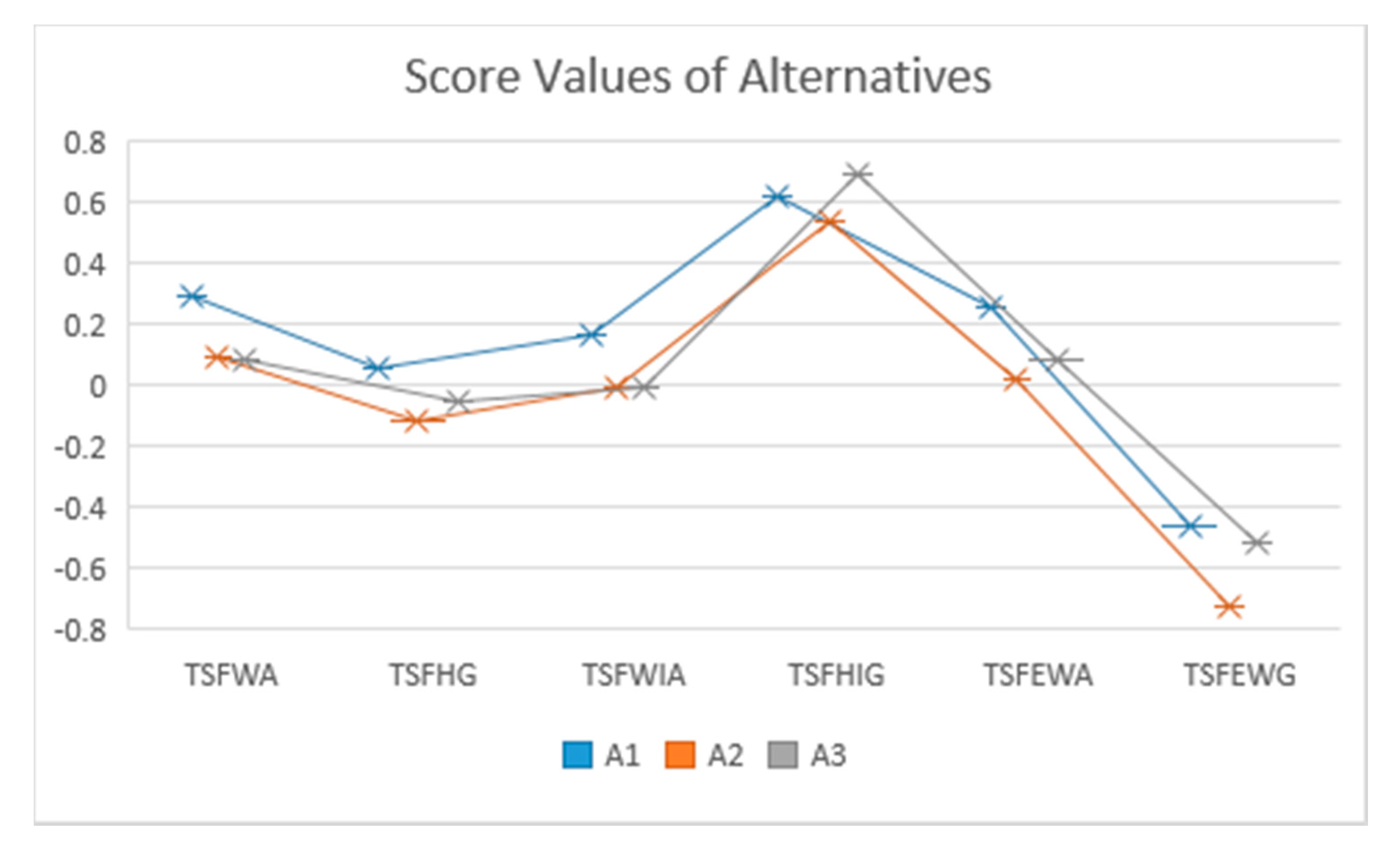
7. Comparative Analysis

In this section, a comparative study is conducted in which it is shown that the proposed operators can be reduced to existing operators under some condition which proves the superiority of the proposed operators. An example is taken from [28] and it is proven that the proposed operators provide the same result.

Consider the T-SFEHA defined as

$$\begin{array}{l}T-SFEH{A}_{\omega ,w}\left({\tilde{P}}_1,{\tilde{P}}_2,\dots ,{\tilde{P}}_k\right)\\ =\left(\begin{array}{c}\sqrt[t]{\frac{{\prod }_{j=1}^k{\left(1+{\tilde{m}}_{\sigma \left(j\right)}^t\right)}^{{\omega }_j}-{\prod }_{j=1}^k{\left(1-{\tilde{m}}_{\sigma \left(j\right)}^t\right)}^{{\omega }_j}}{{\prod }_{j=1}^k{\left(1+{\tilde{m}}_{\sigma \left(j\right)}^t\right)}^{{\omega }_j}+{\prod }_{j=1}^k{\left(1-{\tilde{m}}_{\sigma \left(j\right)}^t\right)}^{{\omega }_j}}}, \sqrt[t]{\frac{2{\prod }_{j=1}^k{({\tilde{i}}_{\sigma \left(j\right)}^t)}^{{\omega }_j}}{{\prod }_{j=1}^k{\left(2-{\tilde{i}}_{\sigma \left(j\right)}^t\right)}^{{\omega }_j}+{\prod }_{j=1}^k{\left({\tilde{i}}_{\sigma \left(j\right)}^t\right)}^{{\omega }_j}}},\\ \sqrt[t]{\frac{2{\prod }_{j=1}^k{({\tilde{n}}_{\sigma \left(j\right)}^t)}^{{\omega }_j}}{{\prod }_{j=1}^k{\left(2-{\tilde{n}}_{\sigma \left(j\right)}^t\right)}^{{\omega }_j}+{\prod }_{j=1}^k{\left({\tilde{n}}_{\sigma \left(j\right)}^t\right)}^{{\omega }_j}}}\end{array}\right)\end{array}$$

• For $t=2$ the above equation reduces to spherical fuzzy Einstein hybrid averaging operators (SFEHA operator), i.e.,

  $$\begin{array}{l}SFEH{A}_{\omega ,w}\left({\tilde{P}}_1,{\tilde{P}}_2,\dots ,{\tilde{P}}_k\right)=\\ \left(\begin{array}{c}\sqrt{\frac{{\prod }_{j=1}^k{\left(1+{\tilde{m}}_{\sigma \left(j\right)}^2\right)}^{{\omega }_j}-{\prod }_{j=1}^k{\left(1-{\tilde{m}}_{\sigma \left(j\right)}^2\right)}^{{\omega }_j}}{{\prod }_{j=1}^k{\left(1+{\tilde{m}}_{\sigma \left(j\right)}^2\right)}^{{\omega }_j}+{\prod }_{j=1}^k{\left(1-{\tilde{m}}_{\sigma \left(j\right)}^2\right)}^{{\omega }_j}}}, \sqrt{\frac{2{\prod }_{j=1}^k{({\tilde{i}}_{\sigma \left(j\right)}^2)}^{{\omega }_j}}{{\prod }_{j=1}^k{\left(2-{\tilde{i}}_{\sigma \left(j\right)}^2\right)}^{{\omega }_j}+{\prod }_{j=1}^k{\left({\tilde{i}}_{\sigma \left(j\right)}^2\right)}^{{\omega }_j}}},\\ \sqrt{\frac{2{\prod }_{j=1}^k{({\tilde{n}}_{\sigma \left(j\right)}^2)}^{{\omega }_j}}{{\prod }_{j=1}^k{\left(2-{\tilde{n}}_{\sigma \left(j\right)}^2\right)}^{{\omega }_j}+{\prod }_{j=1}^k{\left({\tilde{n}}_{\sigma \left(j\right)}^2\right)}^{{\omega }_j}}}\end{array}\right)\end{array}$$
• For $t=1$ the above equation reduces to picture fuzzy Einstein hybrid averaging operators (PFEHA operator), i.e.,

  $$\begin{array}{l}PFEH{A}_{\omega ,w}\left({\tilde{P}}_1,{\tilde{P}}_2,\dots ,{\tilde{P}}_k\right)\\ =\left(\begin{array}{c}\frac{{\prod }_{j=1}^k{\left(1+{\tilde{m}}_{\sigma \left(j\right)}\right)}^{{\omega }_j}-{\prod }_{j=1}^k{\left(1-{\tilde{m}}_{\sigma \left(j\right)}\right)}^{{\omega }_j}}{{\prod }_{j=1}^k{\left(1+{\tilde{m}}_{\sigma \left(j\right)}\right)}^{{\omega }_j}+{\prod }_{j=1}^k{\left(1-{\tilde{m}}_{\sigma \left(j\right)}\right)}^{{\omega }_j}}, \frac{2{\prod }_{j=1}^k{({\tilde{i}}_{\sigma \left(j\right)})}^{{\omega }_j}}{{\prod }_{j=1}^k{\left(2-{\tilde{i}}_{\sigma \left(j\right)}\right)}^{{\omega }_j}+{\prod }_{j=1}^k{\left({\tilde{i}}_{\sigma \left(j\right)}\right)}^{{\omega }_j}},\\ \frac{2{\prod }_{j=1}^k{({\tilde{n}}_{\sigma \left(j\right)})}^{{\omega }_j}}{{\prod }_{j=1}^k{\left(2-{\tilde{n}}_{\sigma \left(j\right)}\right)}^{{\omega }_j}+{\prod }_{j=1}^k{\left({\tilde{n}}_{\sigma \left(j\right)}\right)}^{{\omega }_j}}\end{array}\right)\end{array}$$
• For $i=0$ the above equation reduces to q-ROPF Einstein hybrid averaging operators (q-ROPFEHA operator), i.e.,

  $$\begin{array}{l}q-ROPFEH{A}_{\omega ,w}\left({\tilde{P}}_1,{\tilde{P}}_2,\dots ,{\tilde{P}}_k\right)\\ =\left(\begin{array}{c}\sqrt[t]{\frac{{\prod }_{j=1}^k{\left(1+{\tilde{m}}_{\sigma \left(j\right)}^t\right)}^{{\omega }_j}-{\prod }_{j=1}^k{\left(1-{\tilde{m}}_{\sigma \left(j\right)}^t\right)}^{{\omega }_j}}{{\prod }_{j=1}^k{\left(1+{\tilde{m}}_{\sigma \left(j\right)}^t\right)}^{{\omega }_j}+{\prod }_{j=1}^k{\left(1-{\tilde{m}}_{\sigma \left(j\right)}^t\right)}^{{\omega }_j}}}, \sqrt[t]{\frac{2{\prod }_{j=1}^k{({\tilde{n}}_{\sigma \left(j\right)}^t)}^{{\omega }_j}}{{\prod }_{j=1}^k{\left(2-{\tilde{n}}_{\sigma \left(j\right)}^t\right)}^{{\omega }_j}+{\prod }_{j=1}^k{\left({\tilde{n}}_{\sigma \left(j\right)}^t\right)}^{{\omega }_j}}}\end{array}\right)\end{array}$$
• For $t=2$ and $i=0$ the above equation reduces to PyF Einstein hybrid averaging operators (PyFEHA operator), i.e.,

  $$\begin{array}{l}PyFEH{A}_{\omega ,w}\left({\tilde{P}}_1,{\tilde{P}}_2,\dots ,{\tilde{P}}_k\right)\\ =\left(\begin{array}{c}\sqrt{\frac{{\prod }_{j=1}^k{\left(1+{\tilde{m}}_{\sigma \left(j\right)}^2\right)}^{{\omega }_j}-{\prod }_{j=1}^k{\left(1-{\tilde{m}}_{\sigma \left(j\right)}^2\right)}^{{\omega }_j}}{{\prod }_{j=1}^k{\left(1+{\tilde{m}}_{\sigma \left(j\right)}^2\right)}^{{\omega }_j}+{\prod }_{j=1}^k{\left(1-{\tilde{m}}_{\sigma \left(j\right)}^2\right)}^{{\omega }_j}}}, \sqrt{\frac{2{\prod }_{j=1}^k{({\tilde{n}}_{\sigma \left(j\right)}^2)}^{{\omega }_j}}{{\prod }_{j=1}^k{\left(2-{\tilde{n}}_{\sigma \left(j\right)}^2\right)}^{{\omega }_j}+{\prod }_{j=1}^k{\left({\tilde{n}}_{\sigma \left(j\right)}^2\right)}^{{\omega }_j}}}\end{array}\right)\end{array}$$
• For $t=1$ and $i=0$ the above equation reduces to IF Einstein hybrid averaging operators (IFEHA operator), i.e.,

  $$\begin{array}{l}IFEH{A}_{\omega ,w}\left({\tilde{P}}_1,{\tilde{P}}_2,\dots ,{\tilde{P}}_k\right)\\ =\left(\begin{array}{c}\frac{{\prod }_{j=1}^k{\left(1+{\tilde{m}}_{\sigma \left(j\right)}\right)}^{{\omega }_j}-{\prod }_{j=1}^k{\left(1-{\tilde{m}}_{\sigma \left(j\right)}\right)}^{{\omega }_j}}{{\prod }_{j=1}^k{\left(1+{\tilde{m}}_{\sigma \left(j\right)}\right)}^{{\omega }_j}+{\prod }_{j=1}^k{\left(1-{\tilde{m}}_{\sigma \left(j\right)}\right)}^{{\omega }_j}}, \frac{2{\prod }_{j=1}^k{({\tilde{n}}_{\sigma \left(j\right)})}^{{\omega }_j}}{{\prod }_{j=1}^k{\left(2-{\tilde{n}}_{\sigma \left(j\right)}\right)}^{{\omega }_j}+{\prod }_{j=1}^k{\left({\tilde{n}}_{\sigma \left(j\right)}\right)}^{{\omega }_j}}\end{array}\right)\end{array}$$

  (7)

Similarly, we can reduce the T-SFEWA, T-SFEOWA, T-SFEWG, T-SFEOWG and T-SFEHG operators.

Example 2.

Consider a decision matrix having five alternatives $\left\{{\mathcal{A}}_1, {\mathcal{A}}_2,{\mathcal{A}}_3,{\mathcal{A}}_4,{\mathcal{A}}_5\right\}$ and evaluate under four attributes $\left\{G_1,G_2,G_3,G_4\right\}$

The experts evaluate the alternatives on the basis of given attributes as in

Table 11. Decision Matrix.

	${\mathit{G}}_1$	${\mathit{G}}_2$	${\mathit{G}}_3$	${\mathit{G}}_4$
${\mathcal{A}}_1$	$\left(0.4,0.5\right)$	$\left(0.5,0.4\right)$	$\left(0.2,0.7\right)$	$\left(0.2,0.5\right)$
${\mathcal{A}}_2$	$\left(0.6,0.4\right)$	$\left(0.6,0.3\right)$	$\left(0.6,0.3\right)$	$\left(0.3,0.6\right)$
${\mathcal{A}}_3$	$\left(0.5,0.5\right)$	$\left(0.4,0.5\right)$	$\left(0.4,0.4\right)$	$\left(0.5,0.4\right)$
${\mathcal{A}}_4$	$\left(0.7,0.2\right)$	$\left(0.5,0.4\right)$	$\left(0.2,0.5\right)$	$\left(0.3,0.7\right)$
${\mathcal{A}}_5$	$\left(0.5,0.3\right)$	$\left(0.3,0.4\right)$	$\left(0.6,0.2\right)$	$\left(0.4,0.4\right)$

.

The above decision matrix can be written in the T-SFSs environment as in

Table 12. Decision Matrix in the form of T-SFNs.

	${\mathit{G}}_1$	${\mathit{G}}_2$	${\mathit{G}}_3$	${\mathit{G}}_4$
${\mathcal{A}}_1$	$\left(0.4,0,0.5\right)$	$\left(0.5,0,0.4\right)$	$\left(0.2,0,0.7\right)$	$\left(0.2,0,0.5\right)$
${\mathcal{A}}_2$	$\left(0.6,0,0.4\right)$	$\left(0.6,0,0.3\right)$	$\left(0.6,0,0.3\right)$	$\left(0.3,0,0.6\right)$
${\mathcal{A}}_3$	$\left(0.5,0,0.5\right)$	$\left(0.4,0,0.5\right)$	$\left(0.4,0,0.4\right)$	$\left(0.5,0,0.4\right)$
${\mathcal{A}}_4$	$\left(0.7,0,0.2\right)$	$\left(0.5,0,0.4\right)$	$\left(0.2,0,0.5\right)$	$\left(0.3,0,0.7\right)$
${\mathcal{A}}_5$	$\left(0.5,0,0.3\right)$	$\left(0.3,0,0.4\right)$	$\left(0.6,0,0.2\right)$	$\left(0.4,0,0.4\right)$

with a weighting vector $\omega ={\left(0.2,0.1, 0.3,0.4\right)}^T$. Then, by using Equation (1) we get T-SFEWA values as in

Table 13. T-SFEWA values.

	${\mathit{G}}_1$	${\mathit{G}}_2$	${\mathit{G}}_3$	${\mathit{G}}_4$
${\mathcal{A}}_1$	$\left(0.3265,0,0.5109\right)$	$\left(0.2163,0,0.4814\right)$	$\left(0.2386,0,0.7406\right)$	$\left(0.3135,0,0.4458\right)$
${\mathcal{A}}_2$	$\left(0.5039,0,0.4319\right)$	$\left(0.2704,0,0.4396\right)$	$\left(0.6814,0,0.2548\right)$	$\left(0.4584,0,0.6213\right)$
${\mathcal{A}}_3$	$\left(0.4132,0,0.5109\right)$	$\left(0.1679,0,0.5171\right)$	$\left(0.4687,0,0.3659\right)$	$\left(0.7059,0,0.2975\right)$
${\mathcal{A}}_4$	$\left(0.6004,0,0.2561\right)$	$\left(0.2163,0,0.4814\right)$	$\left(0.2386,0,0.4850\right)$	$\left(0.4584,0,0.8210\right)$
${\mathcal{A}}_5$	$\left(0.4132,0,0.3478\right)$	$\left(0.1232,0,0.4814\right)$	$\left(0.6814,0,0.1535\right)$	$\left(0.5901,0,0.2975\right)$

.

Then, by using score function we order them as listed in

Table 14. Ordered T-SFEWA values.

	${\mathit{G}}_1$	${\mathit{G}}_2$	${\mathit{G}}_3$	${\mathit{G}}_4$
${\mathcal{A}}_{\sigma \left(1\right)}$	$\left(0.3135,0,0.4458\right)$	$\left(0.3265,0,0.5109\right)$	$\left(0.2163,0,0.4814\right)$	$\left(0.2386,0,0.7406\right)$
${\mathcal{A}}_{\sigma \left(2\right)}$	$\left(0.6814,0,0.2548\right)$	$\left(0.5039,0,0.4319\right)$	$\left(0.4584,0,0.6213\right)$	$\left(0.2704,0,0.4396\right)$
${\mathcal{A}}_{\sigma \left(3\right)}$	$\left(0.7059,0,0.2975\right)$	$\left(0.4687,0,0.3659\right)$	$\left(0.4132,0,0.5109\right)$	$\left(0.1679,0,0.5171\right)$
${\mathcal{A}}_{\sigma \left(4\right)}$	$\left(0.6004,0,0.2561\right)$	$\left(0.2386,0,0.4850\right)$	$\left(0.2163,0,0.4814\right)$	$\left(0.4584,0,0.8210\right)$
${\mathcal{A}}_{\sigma \left(5\right)}$	$\left(0.6814,0,0.1535\right)$	$\left(0.5901,0,0.2975\right)$	$\left(0.4132,0,0.3478\right)$	$\left(0.1232,0,0.4814\right)$

:

By using Equation (3), we get

$$\begin{gathered} {\tilde{\mathcal{A}}}_{\sigma \left(1\right)}=\left(0.2434,0,0.5477\right) \\ {\tilde{\mathcal{A}}}_{\sigma \left(2\right)}=\left(0.4534,0,0.4360\right) \\ {\tilde{\mathcal{A}}}_{\sigma \left(3\right)}=\left(0.4273,0,0.4119\right) \\ {\tilde{\mathcal{A}}}_{\sigma \left(4\right)}=\left(0.3109,0,0.5072\right) \end{gathered}$$

The score values of aggregated values will be $SC\left({\tilde{\mathcal{A}}}_{\sigma \left(1\right)}\right)=-0.3043$, $SC\left({\tilde{\mathcal{A}}}_{\sigma \left(2\right)}\right)=-0.0174$, $SC\left({\tilde{\mathcal{A}}}_{\sigma \left(3\right)}\right)=-0.0154$, $SC\left({\tilde{\mathcal{A}}}_{\sigma \left(4\right)}\right)=-0.1964$, $SC\left({\tilde{\mathcal{A}}}_{\sigma \left(5\right)}\right)=-0.1499$.

This shows that is most desirable alternative. Similarly, the above example can be aggregated by using T-SFEHG operator.

Example 3.

Consider the information is given in T-spherical fuzzy environment for $t=3$ as given in

Table 15. Decision Matrix.

	${\mathit{G}}_1$	${\mathit{G}}_2$	${\mathit{G}}_3$	${\mathit{G}}_4$	${\mathit{G}}_5$
$A_1$	$\left(0.5, 0.3,0.4\right)$	$\left(0.9, 0.4,0.5\right)$	$\left(0.7, 0.5,0.2\right)$	$\left(0.8, 0.5,0.5\right)$	$\left(0.2, 0.2,0.8\right)$
$A_2$	$\left(0.2, 0.4,0.7\right)$	$\left(0.4, 0.1,0.2\right)$	$\left(0.9, 0.2,0.5\right)$	$\left(0.3, 0.2,0.6\right)$	$\left(0.5, 0.3,0.7\right)$
$A_3$	$\left(0.6, 0.2,0.4\right)$	$\left(0.3, 0.5,0.7\right)$	$\left(0.7, 0.2,0.4\right)$	$\left(0.5, 0.1,0.2\right)$	$\left(0.4, 0.3,0.5\right)$

:

Then some aggregation operators, e.g., T-spherical fuzzy weighted averaging (T-SFWA) operators, T-spherical fuzzy hybrid geometric (T-SFHG) operators, T-spherical fuzzy weighted interactive averaging (T-SFWIA), T-spherical fuzzy hybrid interactive geometric (T-SFHIG) operators, T-SFEWA operators, and T-SFEWG operators are used to solve given data. The aggregated values for these operators are given in

Table 16. Aggregated values of Table 15.

	T-SFWA Operators [28]	T-SFHG Operators [24]	T-SFWIA Operators [28]	T-SFHIG Operators [24]	T-SFEWA Operators	T-SFEWG Operators
${\mathrm{A}}_1$	$\left(\begin{array}{c}0.7284,\\ 0.3440,\\ 0.4570\end{array}\right)$	$\left(\begin{array}{c}0.5855,\\ 0.3824,\\ 0.5216\end{array}\right)$	$\left(\begin{array}{c}0.7284, \\ 0.3995,\\ 0.6010\end{array}\right)$	$\left(\begin{array}{c}0.9132,\\ 0.7872,\\ 0.5216\end{array}\right)$	$\left(\begin{array}{c}0.6914,\\ 0.3859,\\ 0.4178\end{array}\right)$	$\left(\begin{array}{c}0.6121,\\ 0.8737,\\ 0.8837\end{array}\right)$
${\mathrm{A}}_2$	$\left(\begin{array}{c}0.6015, \\ 0.2264,\\ 0.5039\end{array}\right)$	$\left(\begin{array}{c}0.4723,\\ 0.2102,\\ 0.6030\end{array}\right)$	$\left(\begin{array}{c}0.6015,\\ 0.2927,\\ 0.6121\end{array}\right)$	$\left(\begin{array}{c}0.9111,\\ 0.8905,\\ 0.6030\end{array}\right)$	$\left(\begin{array}{c}0.5182, \\ 0.2182,\\ 0.4960\end{array}\right)$	$\left(\begin{array}{c}0.4325, \\ 0.8056,\\ 0.9297\end{array}\right)$
${\mathrm{A}}_3$	$\left(\begin{array}{c}0.5367,\\ 0.2318,\\ 0.4148\end{array}\right)$	$\left(\begin{array}{c}0.6164,\\ 0.1959,\\ 0.5770\end{array}\right)$	$\left(\begin{array}{c}0.5367,\\ 0.3286,\\ 0.5440\end{array}\right)$	$\left(\begin{array}{c}0.9579,\\ 0.8506,\\ 0.5770\end{array}\right)$	$\left(\begin{array}{c}0.5277,\\ 0.2188,\\ 0.3922\end{array}\right)$	$\left(\begin{array}{c}0.5078, \\ 0.8111,\\ 0.8663\end{array}\right)$

:

The scores of the aggregated data obtained in Table 16 are given in

Table 17. Score Values.

	T-SFWA Operators [28]	T-SFHG Operators [24]	T-SFWIA Operators [28]	T-SFHIG Operators [24]	T-SFEWA Operators	T-SFEWG Operators
${\mathrm{A}}_1$	$0.2909$	$0.0588$	$0.1693$	$0.6196$	$0.2576$	$-0.4608$
${\mathrm{A}}_2$	$0.0897$	$-0.1140$	$-0.0118$	$0.5371$	$0.0172$	$-0.7227$
${\mathrm{A}}_3$	$0.0832$	$-0.0544$	$-0.0064$	$0.6868$	$0.0866$	$-0.5192$

as follows:

The geometrical comparison of the score values obtained using different aggregation techniques is depicted in Figure 2 where the blue stars denote the score values of the $A_1$ using different AOs while the orange and grey stars denote the score values of the alternatives $A_2$ and $A_3$, respectively.

The demonstration of the ranking results observed in Figure 2 are described in

Table 18. Rankings.

Aggregation Operators	Reference	Rankings
T-SFWA operators	Zeng et al. [28]	$A_1>A_2>A_3$
T-SFHG operators	Garg et al. [24]	$A_1>A_3>A_2$
T-SFWIA operators	Zeng et al. [28]	$A_1>A_3>A_2$
T-SFHIG operators	Garg et al. [24]	$A_3>A_1>A_2$
T-SFEWA operators	This Paper	$A_1>A_3>A_2$
T-SFEWG operators	This Paper	$A_1>A_3>A_2$

.

Advantages

The advantages of proposed work over existing work are discussed in this section. The advantages of our work are as follows:

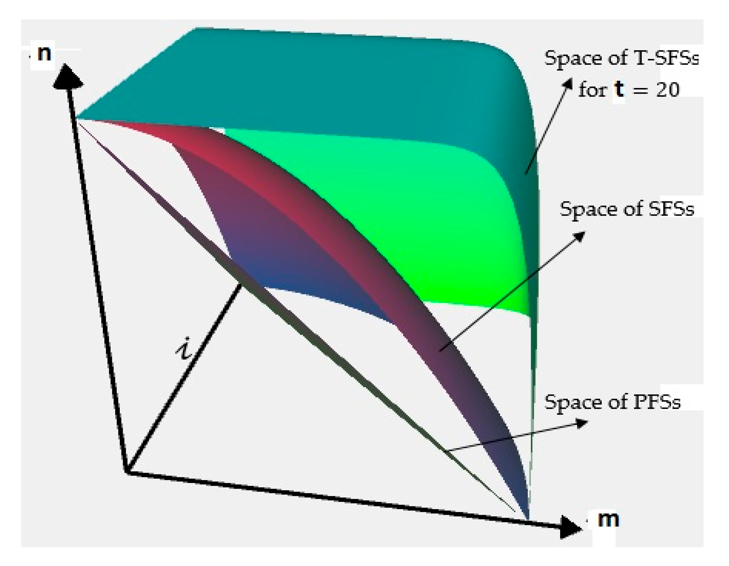
• T-SFS is superior to IFS, PyFS, q-ROPFS, PFS and SFS which is claimed and proved Example 1 and 2.
• T-spherical fuzzy Einstein AOs are more flexible than Einstein aggregation operators of IFSs, PyFSs and, PFS. This flexibility is shown in Section 7 where few restrictions on the proposed operator reduce them to Einstein operators of IFSs, PyFSs, q-ROPFSs, PFSs, and SFSs.
• Proposed operators can solve all the problems that are discussed in [15,17,18,24,25,26,29,40] but the existing operators cannot solve the problems when the information is given in T-SFNs.

8. Conclusions

In this paper, some new Einstein AOs are proposed by pointing out the shortcomings of the existing operators. T-SF Einstein AOs can deal with problems where human opinion is more than two types, i.e., it involves some abstinence and refusal degree as well. Some operations are defined for T-SFSs and based on these operations some improved Einstein averaging aggregation operators and Einstein geometric aggregation operators are defined. Some properties of these aggregation operators are also discussed. The validity of proposed operators is checked with the help of the MADM problem. The comparative analysis between existing and proposed work is also discussed, in which some conditions are studied under which the proposed operators can be reduced to other tools of uncertainty, such as IFSs, PyFSs, q-ROPFSs, PFSs, SFSs. Some examples are also discussed in which the superiority of proposed operators is proved. The advantages of proposed operators are also discussed. In the future, we aim to develop some power AOs, McLaurin symmetric mean operators, Heronian mean AOs and Dombi AOs in the environment of T-SFSs. We also aim to generalize these operators in the field of T-spherical fuzzy soft sets.

References

1. Zadeh, L.A. Fuzzy sets. Inf. Control. 1965, 8, 338–353. [Google Scholar] [CrossRef] [Green Version]
2. Atanassov, K.T. Intuitionistic fuzzy sets. Fuzzy Sets Syst. 1986, 20, 87–96. [Google Scholar] [CrossRef]
3. Yager, R.R. Pythagorean Fuzzy Subsets. In Proceedings of the IFSA World Congress and NAFIPS Annual Meeting (IFSA/NAFIPS), Edmonton, AB, Canada, 24–28 June 2013. [Google Scholar]
4. Yager, R.R. Generalized orthopair fuzzy sets. IEEE Trans. Fuzzy Syst. 2017, 25, 1222–1230. [Google Scholar] [CrossRef]
5. Cuong, B.C. Picture fuzzy sets. J. Comput. Sci. Cybern. 2014, 30, 409. [Google Scholar]
6. Mahmood, T.; Ullah, K.; Khan, Q.; Jan, N. An Approach towards Decision Making and Medical Diagnosis Problems Using the Concept of Spherical Fuzzy Sets. Neural Comput. Appl. 2018, 31, 7041–7053. [Google Scholar] [CrossRef]
7. Bellman, R.E.; Zadeh, L.A. Decision-making in a fuzzy environment. Manag. Sci. 1970, 17, B-141–B-164. [Google Scholar] [CrossRef]
8. Xu, Z. Intuitionistic fuzzy aggregation operators. IEEE Trans. Fuzzy Syst. 2007, 15, 1179–1187. [Google Scholar]
9. Klement, E.P.; Mesiar, E.P. Triangular norms. Position I: Basic analytic and algebraic properties. Fuzzy Sets Syst. 2004, 143, 5–26. [Google Scholar] [CrossRef]
10. Rahman, K.; Ali, A.; Shakeel, M.; Khan, M.; Ullah, M. Pythagorean fuzzy weighted averaging aggregation operator and its application to decision making theory. Nucleus 2017, 54, 190–196. [Google Scholar]
11. Yager, R.R.; Abbasov, A.M. Pythagorean membership grades, complex numbers, and decision making. Int. J. Intell. Syst. 2013, 28, 436–452. [Google Scholar] [CrossRef]
12. Wei, G. Picture fuzzy aggregation operators and their application to multiple attribute decision making. J. Intell. Fuzzy Syst. 2017, 33, 713–724. [Google Scholar] [CrossRef]
13. Garg, H. Some picture fuzzy aggregation operators and their applications to multicriteria decision-making. Arab. J. Sci. Eng. 2017, 42, 5275–5290. [Google Scholar] [CrossRef]
14. Ullah, K.; Hassan, N.; Mahmood, T.; Jan, N.; Hassan, M. Evaluation of investment policy based on multi-attribute decision making using interval-valued T-spherical fuzzy aggregation operators. Symmetry 2019, 11, 357. [Google Scholar] [CrossRef] [Green Version]
15. Ullah, K.; Mahmood, T.; Jan, N. Some Averaging Aggregation Operators for T-Spherical Fuzzy Sets and Their Applications in Multi-Attribute Decision Making. In Proceedings of the International Conference on Soft Computing and Machine Learning (ICSCML), Wuhan, China, 26–28 April 2019. [Google Scholar]
16. Liu, P.; Khan, Q.; Mahmood, T.; Hassan, N. T-spherical fuzzy power Muirhead mean operator based on novel operational laws and their applications in multi-attribute group decision making. IEEE Access 2019, 7, 22613–22632. [Google Scholar] [CrossRef]
17. Garg, H.; Munir, M.; Ullah, K.; Mahmood, T.; Jan, N. Algorithm for T-Spherical Fuzzy Multi-Attribute Decision Making Based on Improved Interactive Aggregation Operators. Symmetry 2018, 10, 670. [Google Scholar] [CrossRef] [Green Version]
18. Quek, S.G.; Selvachandran, G.; Munir, M.; Mahmood, T.; Ullah, K.; Son, L.H.; Thong, P.H.; Kumar, R.; Priyadarshini, I. Multi-Attribute Multi-Perception Decision-Making Based on Generalized T-Spherical Fuzzy Weighted Aggregation Operators on Neutrosophic Sets. Mathematics 2019, 7, 780. [Google Scholar] [CrossRef] [Green Version]
19. Liu, P.; Munir, M.; Mahmood, T.; Ullah, K. Some Similarity Measures for Interval-Valued Picture Fuzzy Sets and Their Applications in Decision Making. Information 2019, 10, 369. [Google Scholar] [CrossRef] [Green Version]
20. Zeng, S.; Hussain, A.; Mahmood, T.; Ali, M.A.; Ashraf, S.; Munir, M. Covering-Based Spherical Fuzzy Rough Set Model Hybrid with TOPSIS for Multi-Attribute Decision-Making. Symmetry 2019, 11, 547. [Google Scholar] [CrossRef] [Green Version]
21. Zeng, S.; Garg, H.; Munir, M.; Mahmood, T.; Hussain, A. A Multi-Attribute Decision Making Process with Immediate Probabilistic Interactive Averaging Aggregation Operators of T-Spherical Fuzzy Sets and Its Application in the Selection of Solar Cells. Energies 2019, 12, 4436. [Google Scholar] [CrossRef] [Green Version]
22. Hussain, A.; Ali, M.I.; Mahmood, T. Pythagorean fuzzy soft rough sets and their applications in decision-making. J. Taibah Univ. Sci. 2020, 14, 101–113. [Google Scholar] [CrossRef] [Green Version]
23. Hussain, A.; Ali, M.I.; Mahmood, T.; Munir, M. q-Rung orthopair fuzzy soft average aggregation operators and their application in multi-criteria decision making. Int. J. Intell. Syst. 2020, 35, 571–599. [Google Scholar] [CrossRef]
24. Zhao, X.; Wei, G. Some intuitionistic fuzzy Einstein hybrid aggregation operators and their application to multiple attribute decision making. Knowl.-Based Syst. 2013, 37, 472–479. [Google Scholar] [CrossRef]
25. Garg, H. Generalized intuitionistic fuzzy interactive geometric interaction operators using Einstein t-norm and t-conorm and their application to decision making. Comput. Ind. Eng. 2016, 101, 53–69. [Google Scholar] [CrossRef]
26. Garg, H. A new generalized pythagorean fuzzy information aggregation using einstein operations and its application to decision making. Int. J. Intell. Syst. 2016, 31, 886–920. [Google Scholar] [CrossRef]
27. Garg, H. Generalised Pythagorean fuzzy geometric interactive aggregation operators using Einstein operations and their application to decision making. J. Exp. Theor. Artif. Intell. 2018, 30, 763–794. [Google Scholar] [CrossRef]
28. Cai, X.; Han, L. Some induced Einstein aggregation operators based on the data mining with interval-valued intuitionistic fuzzy information and their application to multiple attribute decision making. J. Intell. Fuzzy Syst. 2014, 27, 331–338. [Google Scholar] [CrossRef]
29. Xu, Y.; Li, Y.; Wang, H. The induced intuitionistic fuzzy Einstein aggregation and its application in group decision-making. J. Ind. Prod. Eng. 2013, 30, 2–14. [Google Scholar] [CrossRef]
30. Wang, W.; Liu, X. Intuitionistic fuzzy geometric aggregation operators based on Einstein operations. Int. J. Intell. Syst. 2011, 26, 1049–1075. [Google Scholar] [CrossRef]
31. Rashid, S.; Hammouch, Z.; Kalsoom, H.; Ashraf, R.; Chu, Y.M. New Investigation on the Generalized K-Fractional Integral Operators. Front. Phys. 2020, 8, 25. [Google Scholar] [CrossRef]
32. Chu, H.H.; Kalsoom, H.; Rashid, S.; Idrees, M.; Safdar, F.; Chu, Y.M.; Baleanu, D. Quantum Analogs of Ostrowski-Type Inequalities for Raina’s Function correlated with Coordinated Generalized Phi-Convex Functions. Symmetry 2020, 12, 308. [Google Scholar] [CrossRef] [Green Version]
33. Rashid, S.; Kalsoom, H.; Hammouch, Z.; Ashraf, R.; Baleanu, D.; Chu, Y.M. New Multi-Parametrized Estimates Having pth-Order Differentiability in Fractional Calculus for Predominating h-Convex Functions in Hilbert Space. Symmetry 2020, 12, 222. [Google Scholar] [CrossRef] [Green Version]
34. Kalsoom, H.; Rashid, S.; Idrees, M.; Chu, Y.M.; Baleanu, D. Two-Variable Quantum Integral Inequalities of Simpson-Type Based on Higher-Order Generalized Strongly Preinvex and Quasi-Preinvex Functions. Symmetry 2020, 12, 51. [Google Scholar] [CrossRef] [Green Version]
35. Rafeeq, S.; Kalsoom, K.; Hussain, S.; Rashid, S.; Yu-Ming Chu, Y.M. Delay dynamic double integral inequalities on time scales with applications. Adv. Differ. Equ. 2020, 1, 1–32. [Google Scholar] [CrossRef] [Green Version]
36. Kalsoom, H.; Hussain, S.; Rashid, S. Hermite-Hadamard Type Integral Inequalities for Functions Whose Mixed Partial Derivatives Are Co-ordinated Preinvex. Punjab Univ. J. Math. 2020, 52, 63–76. [Google Scholar]
37. Rashid, S.; Jarad, F.; Noor, M.A.; Kalsoom, H.; Chu, Y.M. Inequalities by means of generalized proportional fractional integral operators with respect to another function. Mathematics 2019, 7, 1225. [Google Scholar] [CrossRef] [Green Version]
38. Deng, y.; Kalsoom, H.; Wu, S. Some New Quantum Hermite-Hadamard Type Estimates Within a Class of Generalized (s,m)-Preinvex Functions. Symmetry 2019, 11, 1283. [Google Scholar] [CrossRef] [Green Version]
39. Kalsoom, H.; Hussain, S. Some Hermite-Hadamard type integral inequalities whose $ n $-times differentiable functions are s-logarithmically convex functions. Punjab Univ. J. Math. 2019, 2019, 65–75. [Google Scholar]
40. Kalsoom, H.; Latif, M.A.; Junjua, M.-U.-D.; Hussain, S.; Shahzadi, G. Some (p, q)-Estimates of Hermite--Hadamard-Type Inequalities For Co-ordinated Convex and Quasi-Convex Functions. Mathematics 2019, 8, 683. [Google Scholar] [CrossRef] [Green Version]
41. Kalsoom, H.; Wu, J.; Hussain, S.; Latif, M.A. Simpson’s type inequalities for co-ordinated convex functions on quantum calculus. Symmetry 2019, 11, 768. [Google Scholar] [CrossRef] [Green Version]
42. Zafar, F.; Kalsoom, H.; Hussain, N. Some inequalities of Hermite-Hadamard type for n-times differentiable (ρ, m)-geometrically convex functions. J. Nonlinear Sci. Appl. 2015, 8, 201–217. [Google Scholar] [CrossRef] [Green Version]
Figure 1. Comparison between PFSs, SFSs and T-SFS.
Symmetry 12 00365 g001
Figure 2. Score values of alternatives using different aggregation operators discussed in [24,28].
Symmetry 12 00365 g002