Facial Expression Recognition by Regional Weighting with Approximated Q-Learning

Abstract

Several facial expression recognition methods cluster facial elements according to similarity and weight them considering the importance of each element in classification. However, these methods are limited by the pre-definitions of units restricting modification of the structure during optimization. This study proposes a modified support vector machine classifier called Grid Map, which is combined with reinforcement learning to improve the classification accuracy. To optimize training, the input image size is normalized according to the cascade rules of a pre-processing detector, and the regional weights are assigned by an adaptive cell size that divides each region of the image using bounding grids. Reducing the size of the bounding grid reduces the area used for feature extraction, allowing more detailed weighted features to be extracted. Error-correcting output codes with a histogram of gradient is selected as the classification method via an experiment to determine the optimal feature and classifier selection. The proposed method is formulated into a decision process and solved via Q-learning. To classify seven emotions, the proposed method exhibits accuracies of 96.36% and 98.47% for four databases and Extended Cohn-–Kanade Dataset (CK+), respectively. Compared to the basic method exhibiting a similar accuracy, the proposed method requires 68.81% fewer features and only 66.33% of the processing time.

1. Introduction

Emotion recognition is an important topic in the development of Internet on Things (IoT)-based smart home architecture and assistant services. In human-computer interaction (HCI), the user’s emotional information is an important factor in designing scenarios efficiently and can be obtained through voice or facial expression analysis. Since the publishing of real-time facial expression recognition in video using support vector machines by Michel et al. [1], several methods for Facial Expression Recognition (FER) based on support vector machine (SVM) [2] have been facilitated by additional studies. The significant differences among these methods are principally determined by feature, classifier, and preprocessing methods, and the performance of each is evaluated through classification accuracy using facial expression databases such as the Extended Cohn-–Kanade Dataset (CK+) or Japanese Female Facial Expression (JAFFE).

According to a recent survey [3], another branch of FER studies uses neural networks for the feature and classifier. For example, Action Unit-inspired deep network (AUDN) [4] is a deep neural network with 95.78% classification accuracy for six facial expression classes in the CK+ database. Another study [5] uses multiple binary classifiers comparing one class with six other classes by training the average of neutral-expression images as classification criteria. In a manner similar to that in this study, Yang et al. [6] modified the generative adversarial network (GAN) to estimate the neutral expression of an unknown actor instead of training based on the average image.

The overall flow of our research suggests and validates a Grid Map that replaces the regional weights of facial elements such as facial landmarks (FLs) [7] and facial action units (AUs) [8]. These methods of weighting facial elements have efficiently improved classification accuracy through consideration for importance. However, these studies have a limitation that a human forced definition of clustering rules for each element is required. To overcome these two limitations, our study proposes and adaptively defines the optimal feature extraction cluster according to reward maximization in reinforcement learning. Increasing classification accuracy with efficient feature extraction affects rewards during training. In addition, reinforcement learning has not been attempted for the improvement of facial element weighting efficiency. The application of dynamic programming is considered difficult in this context because the configurations of weighting models cannot be changed by conventional methods. Therefore, our study also includes a validation of whether classification accuracy is affected by the feature detail differences of facial element regions, and we propose a weighting model called Grid Map, which considers differences of details, and we update its values using reinforcement learning. This Grid Map contains a regional distribution of bounding grids and is optimized for maximum accuracy by combining a multiclass-SVM classifier using HOG (histogram of gradients [9])-ECOC (error-correcting output codes [10]) classification as a combining method for reinforcement learning.

2. Classifiers and Reinforcement Learning for Facial Expression Recognition

If more than one class is to be classified, the binary classifier SVM cannot be used by itself, and must instead be combined with a multiclass-SVM such as ECOC. This section introduces the structural differences between the k-Nearest Neighbor (kNN) and ECOC-SVM, the most representative of multi-class classifiers, and predicts their resulting differences in classification accuracy.

2.1. k-Nearest Neighbor (kNN)

kNN is a representative classifier that can classify a variety of elements in addition to vector feature points. In this algorithm, the parameter k is used to set the number of classes in pre-training, and modifying this parameter allows changes to be made to the distance mapping method, such as using Manhattan or Mahalanobis distances instead of Euclidean distances.

$$\mathrm{X}=\left({\mathrm{x}}_1,\dots ,{\mathrm{x}}_{\mathrm{n}}\right),\mathrm{Y}=\left({\mathrm{y}}_1,\dots ,{\mathrm{y}}_{\mathrm{n}}\right).$$

(1)

Assuming a case using a 2D data space with Equation (1) being a set of coordinates, the distance of each mapping method is calculated using one of the following equations.

• Euclidean distance

$${\mathrm{d}}_{\mathrm{eucledean}}=\sqrt{{{\displaystyle \sum }}_{\mathrm{i}=1}^{\mathrm{n}}{\left({\mathrm{x}}_{\mathrm{i}}-{\mathrm{y}}_{\mathrm{i}}\right)}^2}.$$

(2)

• Manhattan distance

$${\mathrm{d}}_{\mathrm{manhattan}}={{\displaystyle \sum }}_{\mathrm{i}=1}^{\mathrm{n}}\left|{\mathrm{x}}_{\mathrm{i}}-{\mathrm{y}}_{\mathrm{i}}\right|.$$

(3)

• Mahalanobis distance

$${\mathrm{d}}_{\mathrm{mahalanobis}}=\sqrt{{\left(\overrightarrow{\mathrm{x}}-\overrightarrow{\mathrm{y}}\right)}^{\mathrm{T}}{\mathrm{S}}^{-1}{\left(\overrightarrow{\mathrm{x}}-\overrightarrow{\mathrm{y}}\right)}^{}},\mathrm{where}\mathrm{S}\mathrm{is}\mathrm{the}\mathrm{covariance}.$$

(4)

Equation (2) calculates linear distance, whereas Equation (3) calculates the sum of the distances on each axis as the distance between two data sets. Equation (4) calculates the variance and covariance values in the data space as the distance between the data.

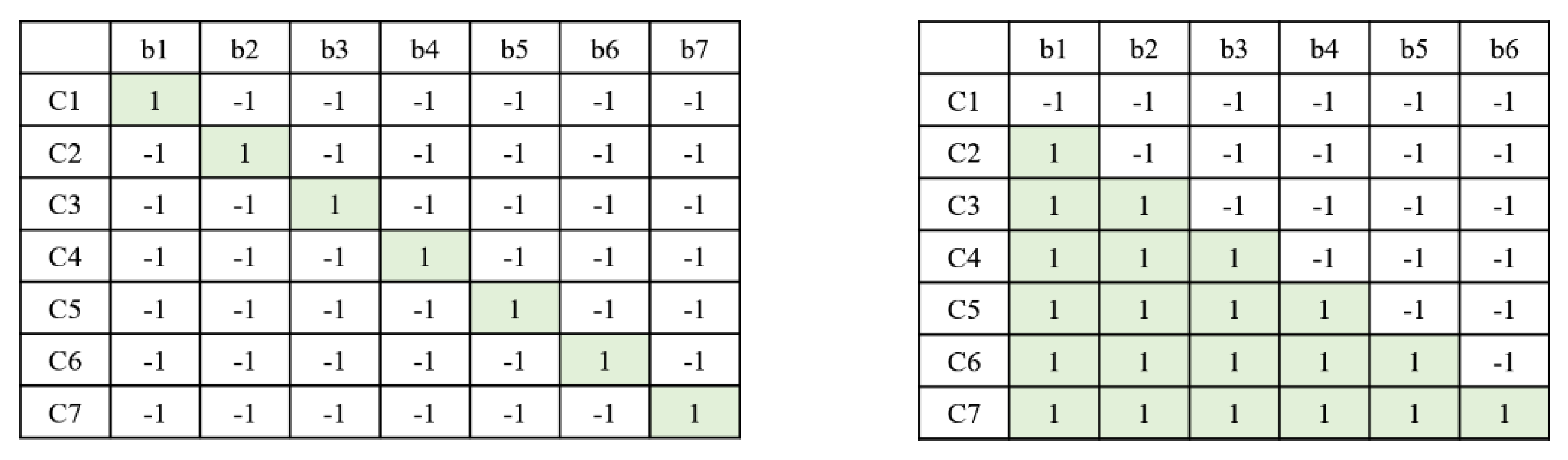
2.2. Error-Correcting Output Codes (ECOC) for Multi-Class SVM

For multi-class classification using a binary SVM classifier, Fei et al. [11] proposed the Binary Tree of Support vector machine (BTS), in which classifiers are connected to a tree as nodes. We selected ECOC [10] as a solution for combining with SVM. ECOC generally uses one of three methods that differ based on the number of nodes and the configuration of the tree, and include one vs. one (OVO), one vs. all (OVA), and ordinal methods. Übeyli et al. [12] compared the accuracy of each tree construction method as applied to SVM, and the experimental result showed the OVO ECOC method to have the highest accuracy among the three methods. The definitions of the three methods are as follows.

One vs. One: k(k-1)/2 nodes, True: 1, False: -1, do not classify: 0.

One vs. All: k nodes, True: 1, False: -1.

Ordinal: k-1 nodes, True: -1, False: 1.

Each SVM connects to subsequent nodes based on a true or false boolean operation. In the case of OVA and ordinal methods, nodes connected to each modified SVM classify a class and all other classes, whereas OVO consists of nodes classifying a class and one other class.

Figure 1 shows the bit composition of the OVA and ordinal methods for a seven-class problem. In the case of the OVA, each bin (b) corresponds to an SVM classifier, which returns a value of 1 for the target class (pertaining to true) and -1 for the other classes (pertaining to false). In the case of the ordinal method, a combination of returns pertaining to b1–b6 is used to make the decision to classify the classes. The OVA consists of k SVM classifiers, and the ordinal reduces the number of bins by 1 through a modified sorting order.

Figure 2 shows OVO consisting of k (k-1)/2 SVM classifiers of a class and another class. Because it is a one-to-one classifier, a value of 0 is returned when not classifying a bin, which is not necessary in the OVA and ordinal methods. Although OVO involves more SVM training stages than the other two methods, it has higher classification accuracy and fewer training images in a given stage.

2.3. Reinforcement Learning

2.3.1. Markov Decision Process (MDP)

MDP [13] is a discrete-time probabilistic control process that consists of a state ($\mathrm{s}$) and an action ($\mathrm{a}$) used to transition from the state ($\mathrm{s}$) to another state (${\mathrm{s}}^{\prime }$). Each reward (${\mathrm{R}}_{\mathrm{a}}\left(\mathrm{s},{\mathrm{s}}^{\prime }\right)$) of the processes is computed according to the purpose of the transition and is derived to maximize compensation. Therefore, the current state ($\mathrm{s}$) is determined by the expected reward for the next state (${\mathrm{s}}^{\prime }$) and its transition (a), giving MDP a probability-independent Markov property [14] that is independent of past processes because it is only affected by the current state (s) and behavior (a).

2.3.2. Reinforcement Learning for MDP Optimization

The purpose of reinforcement learning is to optimize the policy (π), which is the set of all transition stages of the MDP. In other words, it means that the derivation of policy π is intended to obtain the highest cumulative reward starting from the initial state $s_0$ under the assumption that the set of states (S) is finite. The observation of the total cumulative reward can be obtained from Equation (5).

$${\displaystyle \sum }_{\mathrm{t}=0}^{\mathrm{n}}{\mathsf{\gamma }}^{\mathrm{t}}{\mathrm{R}}_{\mathsf{\pi }\left({\mathrm{s}}_{\mathrm{t}}\right)}\left({\mathrm{s}}_{\mathrm{t}},{\mathrm{s}}_{\mathrm{t}+1}\right)=\mathrm{E}\left[\mathrm{R}\left({\mathrm{s}}_0,{\mathrm{s}}_1\right)+\dots +{\mathsf{\gamma }}^{\mathrm{n}}\mathrm{R}\left({\mathrm{s}}_{\mathrm{n}-1},{\mathrm{s}}_{\mathrm{n}}\right)\right].$$

(5)

where t is the policy level and increases by 1 whenever the state ${\mathrm{s}}_{\mathrm{t}}$ transitions to the next state ${\mathrm{s}}_{\mathrm{t}+1}$. γ is a discount factor between [0, 1] that decreases the reward as the step distance of transition (t) increases between the current stage and those in the future. Thus, longer step distances result in the reward being decreased by the exponent of γ, and this discounting can be used to derive a more concise policy. The algorithm consists of updating the policy (π) by recursively repeating this process.

$$\mathsf{\pi }\left(\mathrm{s}\right):=\arg \underset{\mathrm{a}}{\max }\left\{{\displaystyle \sum }_{{\mathrm{s}}^{\prime }}{\mathrm{P}}_{\mathrm{a}}\left(\mathrm{s},{\mathrm{s}}^{\prime }\right)\left({\mathrm{R}}_{\mathrm{a}}\left(\mathrm{s},{\mathrm{s}}^{\prime }\right)+\mathsf{\gamma }\mathrm{V}\left({\mathrm{s}}^{\prime }\right)\right)\right\}.$$

(6)

Equation (6) is the definition of an optimized policy according to a current state (s). The transition probability function ${\mathrm{P}}_{\mathrm{a}}\left(\mathrm{s},{\mathrm{s}}^{\prime }\right)$ represents the probability of transition for the following states and considers all ${\mathrm{s}}^{\prime }$ whose value is non-zero as the next transitionable state. ${\mathrm{R}}_{\mathrm{a}}\left(\mathrm{s},{\mathrm{s}}^{\prime }\right)$ is the reward for each action (a) from the current state (s) to all the possible next states ${\mathrm{s}}^{\prime }$. $\mathrm{V}\left({\mathrm{s}}^{\prime }\right)$ is the expectation of reward value in the future, which is the sum of the reward values when the optimal policy is defined in the current state, and can be written as

$$\mathrm{V}\left(\mathrm{s}\right):={\displaystyle \sum }_{{\mathrm{s}}^{\prime }}{\mathrm{P}}_{\mathsf{\pi }\left(\mathrm{s}\right)}\left(\mathrm{s},{\mathrm{s}}^{\prime }\right)\left({\mathrm{R}}_{\mathsf{\pi }\left(\mathrm{s}\right)}\left(\mathrm{s},{\mathrm{s}}^{\prime }\right)+\mathsf{\gamma }\mathrm{V}\left({\mathrm{s}}^{\prime }\right)\right).$$

(7)

Equation (7) is derived from Equation (6) by summing reward values up to the current state of the policy ($\mathsf{\pi }\left(\mathrm{s}\right)$) discounted by γ. The training iteration is repeated by two recursive equations until it is terminated by a discount factor of zero or a separate learning rate factor ∆L to optimize the policy.

2.3.3. Q-Learning

Q-learning is a method of reinforcement learning which modifies the decision process to optimize the policy. Q-value iteration is used for its recursive repetition. Value iteration and policy iteration are prior iteration methods that can be explained as follows.

• Value iteration

Value Iteration is a method that eliminates the term π(s) for a policy. The value function is given by substituting Equation (6) into Equation (7) and can be written as

$${\mathrm{V}}_{\mathrm{i}+1}\left(\mathrm{s}\right):=\underset{\mathrm{a}}{\max }\left\{{\displaystyle \sum }_{{\mathrm{s}}^{\prime }}{\mathrm{P}}_{\mathrm{a}}\left(\mathrm{s},{\mathrm{s}}^{\prime }\right)\left({\mathrm{R}}_{\mathrm{a}}\left(\mathrm{s},{\mathrm{s}}^{\prime }\right)+\mathsf{\gamma }\mathrm{V}\left({\mathrm{s}}^{\prime }\right)\right)\right\}.$$

(8)

Equation (8) was proposed by Shapley [15] as a stochastic game. Assuming the equation continues to be calculated, the difference between the left and right sides approaches zero, and the reward ${\mathrm{R}}_{\mathrm{a}}\left(\mathrm{s},{\mathrm{s}}^{\prime }\right)$ converges to zero after additional iterations. The initial ${\mathrm{V}}_0\left(\mathrm{s}\right)$ is set to zero or a random value, and i is the number of iterations. The definition of the optimal policy (${\mathsf{\pi }}^{*}\left(\mathrm{s}\right)$) is given by substituting the value function $\mathrm{V}\left(\mathrm{s}\right)$ into optimal value ${\mathrm{V}}^{*}\left(\mathrm{s}\right)$, and it can be written as

$$\begin{gathered} {\pi }^{*}\left(s\right)= \mathbf{arg}\underset{a}{\mathbf{max}}\left\{{{\displaystyle \sum }}_{s^{\prime }}{P}_a\left(s,s^{\prime }\right)\left(R_a\left(s,s^{\prime }\right)+ \gamma V^{*}\left(s^{\prime }\right)\right)\right\}\mathbf{,} \mathrm{where} R_a\left(s,s^{\prime }\right)\approx 0, \\ {\mathsf{\pi }}^{*}\left(\mathrm{s}\right)=\arg \underset{\mathrm{a}}{\max \mathsf{\gamma }}{\displaystyle \sum }_{{\mathrm{s}}^{\prime }}{\mathrm{P}}_{\mathrm{a}}\left(\mathrm{s},{\mathrm{s}}^{\prime }\right){\mathrm{V}}^{*}\left({\mathrm{s}}^{\prime }\right). \end{gathered}$$

(9)

• Policy iteration

Whereas value iteration optimizes V(s) and obtains an optimal policy through Equation (9), policy iteration recursively updates the policy itself. The recursive formula of policy iteration can be written as

$$\mathsf{\pi }\left(\mathrm{s}\right)=\arg \underset{\mathrm{a}}{\max \mathsf{\gamma }}{\displaystyle \sum }_{{\mathrm{s}}^{\prime }}{\mathrm{P}}_{\mathrm{a}}\left(\mathrm{s},{\mathrm{s}}^{\prime }\right)\mathrm{V}\left(\mathrm{s}\right).$$

(10)

where s is the current state, ${\mathrm{s}}^{\prime }$ is any state that can be selected by policy ${\mathrm{P}}_{\mathrm{a}}\left(\mathrm{s},{\mathrm{s}}^{\prime }\right)$, and a is all available actions according to the policy.

• Q-learning [16]

If the reward is different for each V(s) according to the policy, the value function V(s) can be replaced with Q (s, a) for state and behavior. The definition of the Q-function is given as

$$\mathrm{Q}\left(\mathrm{s},\mathrm{a}\right):={\mathrm{P}}_{\mathrm{a}}\left(\mathrm{s},{\mathrm{s}}^{\prime }\right)\left(\mathrm{R}\left(\mathrm{s},{\mathrm{s}}^{\prime }\right)+\mathsf{\gamma }\mathrm{V}\left({\mathrm{s}}^{\prime }\right)\right).$$

(11)

In Equation (11), basic value iteration is used, but the Q-function is recursively updated instead of V(s). The optimal policy of Q-learning can be written as

$${\mathsf{\pi }}^{*}\left(\mathrm{s}\right)=\arg \underset{\mathrm{a}}{\max }\left[\mathrm{r}\left(\mathrm{s},\mathrm{a}\right)+{\mathsf{\gamma }\mathrm{V}}^{*}\left(\mathrm{s},\mathrm{a}\right)\right]=\arg \underset{\mathrm{a}}{\max }\mathrm{Q}\left(\mathrm{s},\mathrm{a}\right).$$

(12)

Equation (12) indicates that Q-learning can be designed to be affected only by each state (s) and action (a). In other words, Q-learning can optimize the policy without a specific behavioral environment model. In its iteration, the optimal Q-function is updated by Equation (13), which is derived from Equation (11), and is given as

$$\mathrm{Q}\left({\mathrm{s}}_{\mathrm{t}},{\mathrm{a}}_{\mathrm{t}}\right)\leftarrow \left(1-\mathsf{\alpha }\right)\mathrm{Q}\left({\mathrm{s}}_{\mathrm{t}},{\mathrm{a}}_{\mathrm{t}}\right)+{\mathsf{\alpha }\mathrm{r}}_{\mathrm{t}}+\mathsf{\gamma }\underset{\mathrm{a}}{\max }\mathrm{Q}\left({\mathrm{s}}_{\mathrm{t}+1},\mathrm{a}\right).$$

(13)

In Equation (13), $\mathrm{s}\to {{\mathrm{t}}^{\prime }\mathrm{s}}_{\left(\mathrm{t}+1\right)}$ replaces $\mathrm{s}\to {\mathrm{s}}^{\prime }$ as the relationship between the current state and the next state. Alpha (α) is a learning rate factor, which decreases as learning progresses and increases the influence of the Q-function $\mathrm{Q}\left({\mathrm{s}}_{\mathrm{t}},{\mathrm{a}}_{\mathrm{t}}\right)$ on future decisions.

3. Facial Expression Recognition by Regional Weighting

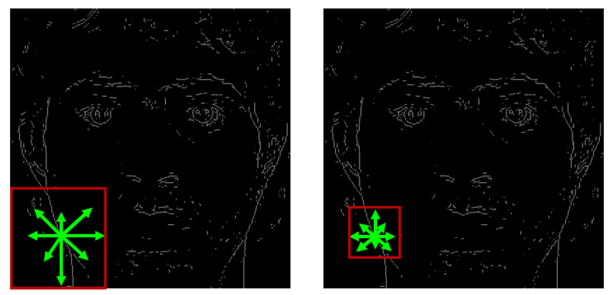
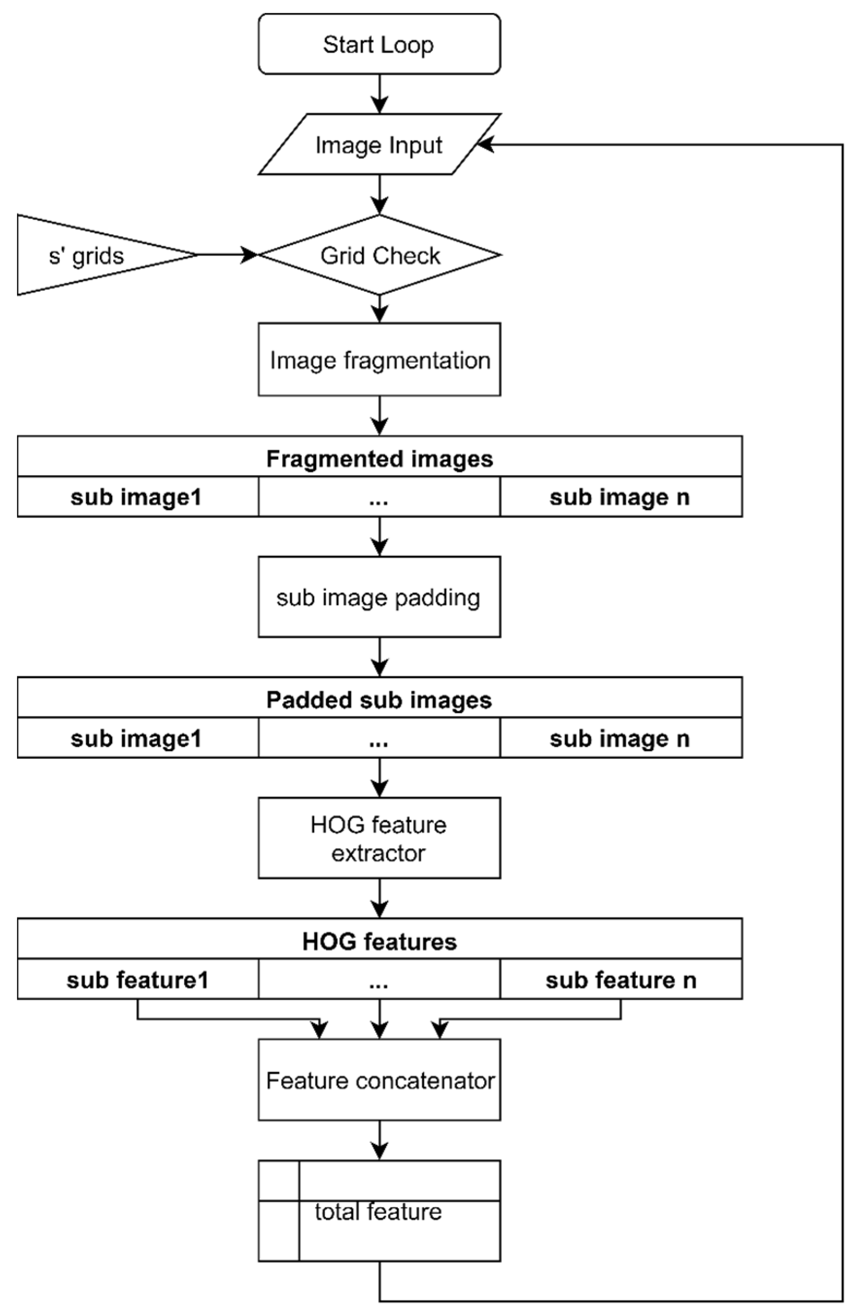
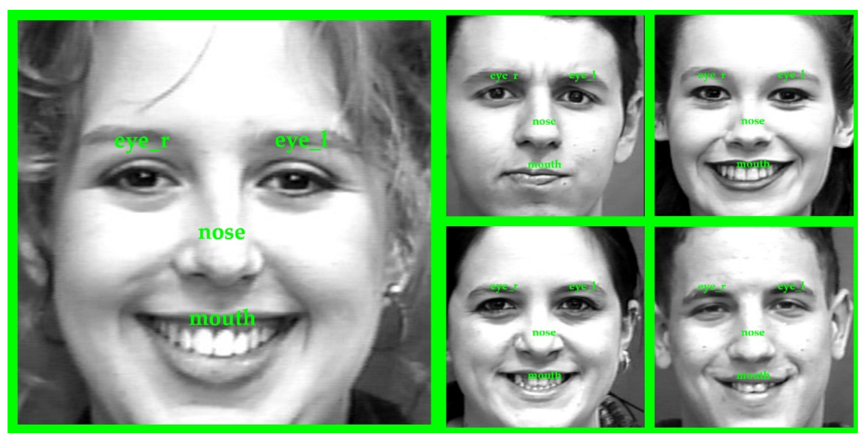
3.1. Feature Extraction by Regional Weighting

Regional weighting is proposed in this paper and gives weights using detail depth in the feature extraction step rather than applying numerical weights to the training stage of classifiers.

Figure 3 shows that even when using the same feature center point, the magnitude in each direction of the extracted feature can be different according to the cell size. This difference is caused by the size of the coverage area used, as the cell size determines the amount of surrounding information included in the computation of the feature. Therefore, a smaller cell size can emphasize a response to changes in detail, but at the cost of increasing the number of feature center points. Grid Map is proposed to modify the conventional feature extractor for optimization by changing the distribution of cells based on differences of classification accuracy.

Figure 4 (right) shows an example of HOG feature extraction using Grid Map. This configuration is an ideal shape for our approach, and the optimized configuration will be shown in the experimental results in Section 4. Basically, the HOG feature points extracted from the image are trained as a matrix after enumerating the features from each cell. When all cells have the same size as shown in the Figure 4 (left), the bins set extracted by each cell is defined as $\mathrm{H}\_\mathrm{k}$ where the total number of cells is k. The total HOG feature matrix in one image is defined as follows in Equation (14).

$${\displaystyle \sum }\mathrm{H}:={\left({\mathrm{H}}_1^{\mathrm{T}},{\mathrm{H}}_2^{\mathrm{T}},\dots ,{\mathrm{H}}_{\mathrm{k}}^{\mathrm{T}}\right)}^{\mathrm{T}},\mathrm{where}{\mathrm{H}}_{\mathrm{k}}\ni \left\{{\mathrm{b}}_1,\dots ,{\mathrm{b}}_{\mathrm{n}}\right\}.$$

(14)

${\mathrm{H}}_{\mathrm{k}}$ in Equation (14) is the set of all bins created in one cell. When learning more than one image, the conventional method is to train the SVM by generating a two-dimensional matrix by enumerating the sets.

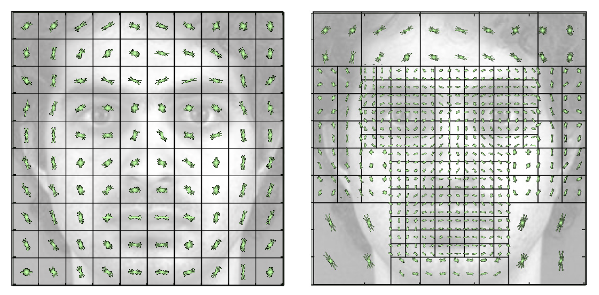
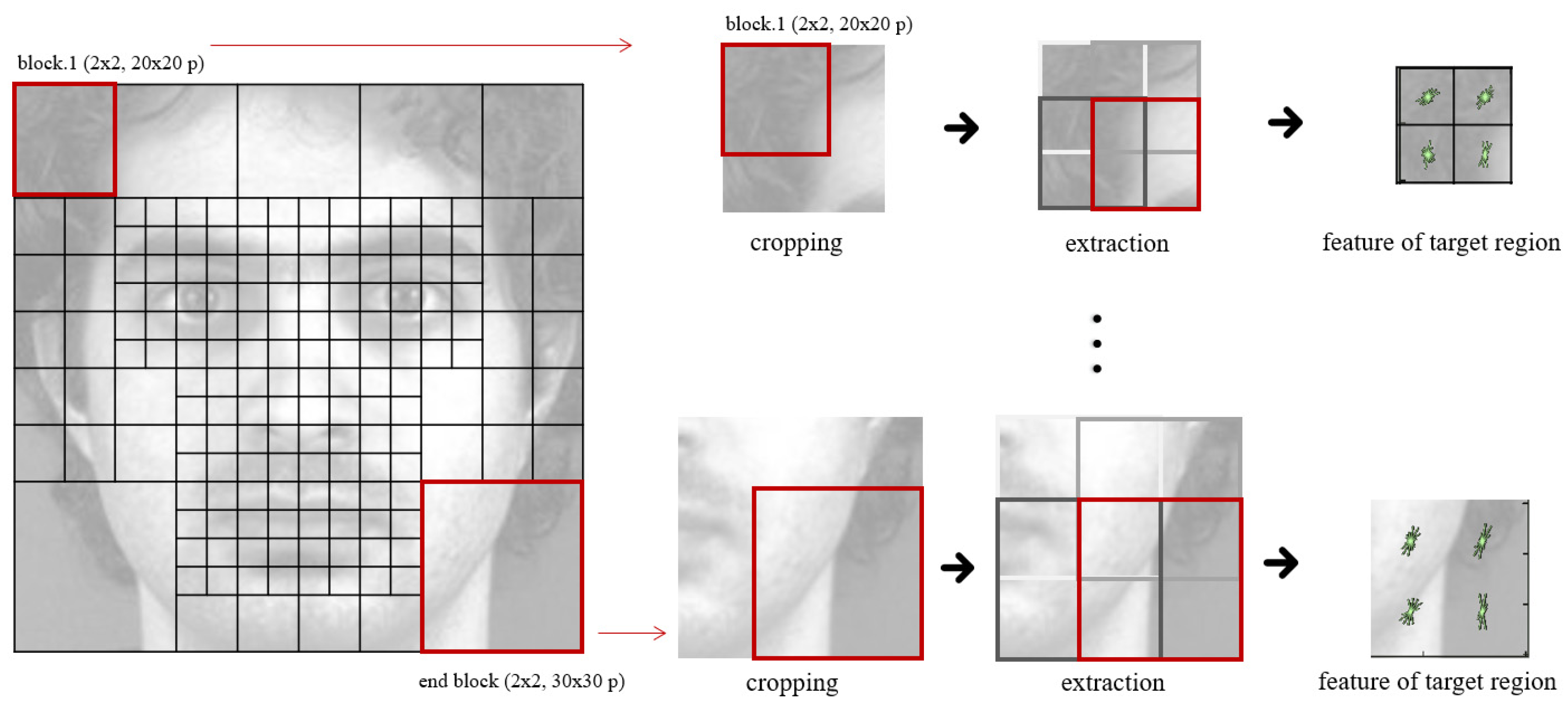
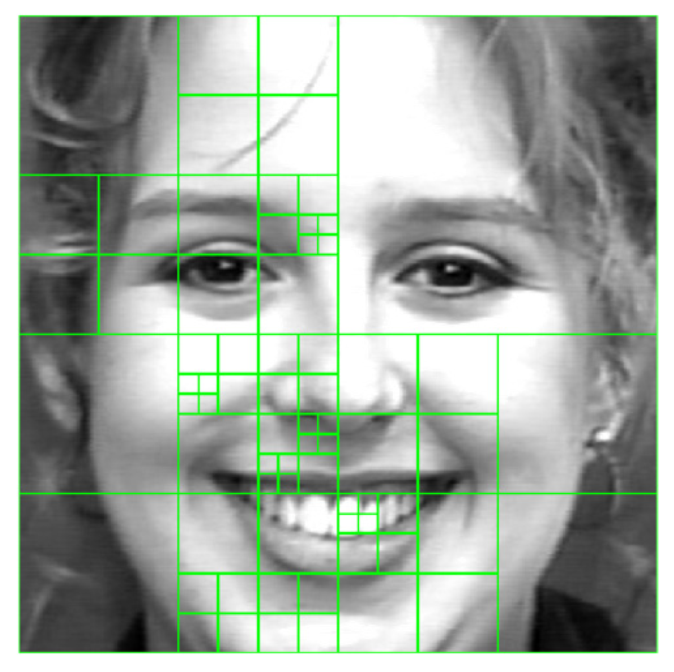
3.2. Vector Feature Extraction Method Using Grid Map

Grid maps have different cell size values for each region of an image. In other words, the size of the region is equal to the size of the cell. The HOG feature extraction parameters include cell size, block size, and overlap ratio, and overlap is a process added to compensate for the shortcomings of non-contiguous feature extractors by crossing neighboring blocks by a specified ratio after feature extraction for each block. In this example, the block size is 2 × 2 and the overlap ratio is fixed at 0.5. The cell size is then adaptively set to generate a square center matrix of size 2 for each area of the Grid Map. In this case, the number of bins (n) can be computed and written as

$${\mathrm{N}}_{\mathrm{b}}:={\mathrm{N}}_{\mathrm{center}}+4{\mathrm{N}}_{\mathrm{overlap}}.$$

(15)

${\mathrm{N}}_{\mathrm{b}}$ is the total number of bins created in one cell, ${\mathrm{N}}_{\mathrm{center}}$ is the number of bins generated from one feature center point,${\mathrm{N}}_{\mathrm{overlap}}$ is the number of bins generated due to overlap, and ${\mathrm{N}}_{\mathrm{gradient}}$ is the number of directions used by HOG. From this, the computation of the number of bins given in Equation (15) can be rewritten as

$${\mathrm{N}}_{\mathrm{center}}:={\mathrm{N}}_{\mathrm{gradient}}\times {\mathrm{c}}^2,$$

(16)

$${\mathrm{N}}_{\mathrm{overlap}}:={\mathrm{N}}_{\mathrm{gradient}}\times \left(0.5\mathrm{c}-1\right)\left(1.5\mathrm{c}-1\right).$$

(17)

${\mathrm{N}}_{\mathrm{gradient}}$ is the number of feature extractor directions, and c is the cell size. In other words, both Equation (16) and Equation (17) consist of only one variable c. Substituting this in the following Equation (18) is finally derived as

$${\mathrm{N}}_{\mathrm{b}}={\mathrm{N}}_{\mathrm{gradient}}\times \left({\mathrm{c}}^2+4\left(0.5\mathrm{c}-1\right)\left(1.5\mathrm{c}-1\right)\right).$$

(18)

In all Grid Map areas, Equation (18) is implemented as the constant c, because the size of the center matrix is fixed to 2. Assuming the number of feature center points to be extracted is the same, the number of feature points to be extracted is the same. Therefore, bin sets of HOGs extracted from regions having different sizes can be enumerated in a matrix ${\mathrm{H}}^{*}$.

$${\mathrm{H}}^{*}={\left({\mathrm{H}}_1^{\mathrm{T}},{\mathrm{H}}_2^{\mathrm{T}},\dots ,{\mathrm{H}}_{\mathrm{k}}^{\mathrm{T}}\right)}^{\mathrm{T}}.$$

(19)

Equation (19) yields all features of an image when the number of grids is k. Therefore, HOG features extracted from different sizes of ${\displaystyle \sum }{\mathrm{H}}^{*}$ are collected in the same form as ${\displaystyle \sum }\mathrm{H}$ of the conventional method, which means that can be trained by SVM.

3.3. Weighted Feature Extraction with Grid Map

The existing HOG feature extraction has an overlap stage to compensate for the skipping caused by the characteristics of discontinuous feature extractors. To prevent this problem, overlap is replaced with a padding stage to consider neighboring region by extending each cell size by half.

Figure 5 illustrates how the features were extracted as an order of Grid Map. After cropping the image of each region, set the cell size to 2 × 2 for feature point extraction. In the cropping phase, the area padding is shown by the crossing rate of 0.5. Every region has four feature points regardless of the resolution, and the merged feature matrix of each region is used in training as a single feature set of an image. The flow chart of this algorithm is shown in Figure 6 below.

Figure 6 shows the feature extraction and merging process of an image using the Grid Map corresponding to the current state (s’). The total features of a merged matrix can be computed via Equation (18) as $\mathrm{n}\left(32\mathrm{bins}+4\mathrm{centers}\right)$.

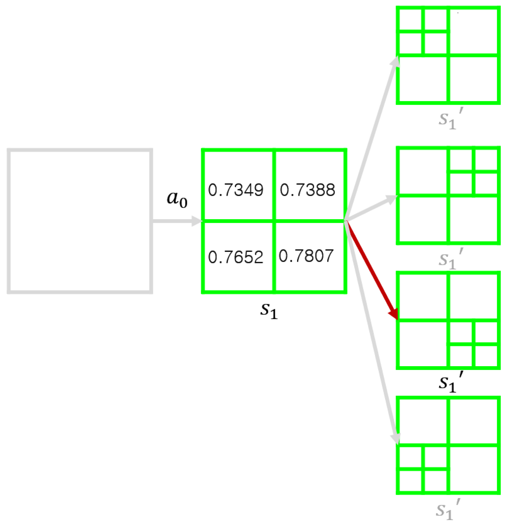
3.4. Combining with Reinforcement Learning

Grid Map G consists of grids with n boxes B that split the area for the specified learning image size.

$$\mathrm{G}\ni \{{\mathrm{B}}_1,{\mathrm{B}}_2,\dots ,{\mathrm{B}}_{\mathrm{n}}\}.$$

(20)

For the initial stage of Equation (20), there is only one grid, with n = 1, and it is illustrated as Figure 7.

3.4.1. One-Way Decision Process

In the state ${\mathrm{s}}_0$ of Figure 7, there are two valid actions, one of which is to maintain ${\mathrm{s}}_0$, and the other is to split its grid and transition to ${{\mathrm{s}}_0}^{\prime }$. In this situation, the reward that can be given is defined as an improvement in accuracy when the Grid Map is transitioned by action. Accordingly, the rewards for each state can be written as

$$\mathrm{V}\left({\mathrm{s}}_0\right)=\arg \underset{\mathrm{a}}{\max }\{\mathrm{R}\left({\mathrm{s}}_0,{\mathrm{s}}_0^{\prime }\right)\}=\underset{\mathrm{a}}{\max }\left\{\mathrm{A}\left({\mathrm{s}}_0^{\prime }\right)-\mathrm{A}\left({\mathrm{s}}_0\right),\mathrm{A}\left({\mathrm{s}}_0\right)-\mathrm{A}\left({\mathrm{s}}_0\right)\right\}.$$

(21)

Assuming the transition probabilities are the same, Equation (21) represents the value of $\mathrm{V}\left(\mathrm{s}\right)$. Because the accuracy of ${{\mathrm{s}}_0}^{\prime }$ was higher in later experiments, the reward by splitting is $\mathrm{R}\left({\mathrm{s}}_0,{\mathrm{s}}_0^{\prime }\right)>0$, and at splitting, $\mathrm{R}\left({\mathrm{s}}_0,{\mathrm{s}}_0\right)=\mathrm{A}\left({\mathrm{s}}_0\right)-\mathrm{A}\left({\mathrm{s}}_0\right)=0$. In this situation, the change to the Grid Map can written as

$$\mathrm{G}\left({\mathrm{s}}_0\right)\ni \left\{{\mathrm{B}}_1\right\}.$$

(22)

Equation (22) represents the Grid Map for ${\mathrm{s}}_0$. When ${\mathrm{s}}_0\to {\mathrm{s}}_1$ transition, ${\mathrm{B}}_1$ is replaced with a set ${\mathrm{B}}_1^{\prime }\ni \left\{{\mathrm{B}}_1,{\mathrm{B}}_2,{\mathrm{B}}_3,{\mathrm{B}}_4\right\}$ containing four split grids to update the Grid Map with the following equation.

$$\mathrm{G}\left({\mathrm{s}}_1\right)\ni \{{\mathrm{B}}_1,{\mathrm{B}}_2,{\mathrm{B}}_3,{\mathrm{B}}_4\}.$$

(23)

In Equation (23), the number of grids is increased by 3 through one transition, and then the number of grids is increased by 3 each time the split action is selected.

3.4.2. Multi-Way Decision Process

In the next iteration, ${\mathrm{s}}_0^{\prime }$ becomes s_1 and represents states that can be transitioned, as shown in Figure 8.

In Figure 8, there are five transitional states including four partitions and one hold. The values displayed in each grid represent the accuracy of classification in adaptive feature extraction using the Grid Map as it is updated by the selected behavior. Because the reward value of a maintained state is zero, this state will transition to a grid that returns the highest accuracy of the four splitting actions.

3.5. Q-Function Definition for Optimizing

The observed Q-function can be derived from a formula of A(s) and R(s) in Equation (21) that contributes to the reward from validation, and it can be written as

$$\mathrm{Q}\left(\mathrm{s},\mathrm{a}\right)=\mathrm{E}\left[\mathrm{R}\left({\mathrm{s}}_0,{\mathrm{a}}_0\right)+\mathsf{\gamma }\mathrm{R}\left({\mathrm{s}}_1,{\mathrm{a}}_1\right)+\dots +{\mathsf{\gamma }}^{\mathrm{n}}\mathrm{R}\left({\mathrm{s}}_{\mathrm{n}},{\mathrm{a}}_{\mathrm{n}}\right)\right].$$

(24)

Considering the relationship of $\mathrm{R}\left(\mathrm{s},\mathrm{a}\right)=\mathrm{A}\left({\mathrm{s}}^{\prime }\right)-\mathrm{A}\left(\mathrm{s}\right)$ described in Equation (24), the observation of the Q-function can be written as

$$\mathrm{Q}\left(\mathrm{s},\mathrm{a}\right)=\mathrm{E}\left[\mathrm{A}\left({\mathrm{s}}_1\right)-\mathrm{A}\left({\mathrm{s}}_0\right)+\mathsf{\gamma }\mathrm{A}\left({\mathrm{s}}_2\right)-\mathsf{\gamma }\mathrm{A}\left({\mathrm{s}}_1\right)+\dots +{\mathsf{\gamma }}^{\mathrm{n}}\mathrm{A}\left({\mathrm{s}}_{\mathrm{n}}\right)-{\mathsf{\gamma }}^{\mathrm{n}}\mathrm{A}\left({\mathrm{s}}_{\mathrm{n}-1}\right)\right]$$

$$=\mathrm{E}\left[{\mathsf{\gamma }}^{\mathrm{n}}\mathrm{A}\left({\mathrm{s}}_{\mathrm{n}}\right)-\mathrm{A}\left({\mathrm{s}}_0\right)+\left(1-\mathsf{\gamma }\right)\mathrm{A}\left({\mathrm{s}}_1\right)+\mathsf{\gamma }\left(1-\mathsf{\gamma }\right)\mathrm{A}\left({\mathrm{s}}_2\right)+\dots +{\mathsf{\gamma }}^{\mathrm{n}-1}\left(1-\mathsf{\gamma }\right)\mathrm{A}\left({\mathrm{s}}_{\mathrm{n}}\right)\right].$$

(25)

Equation (25) means that the Q-function depends only on accuracy $\mathrm{A}\left(\mathrm{s}\right)$ at time ($\mathrm{t}$). The discount factor γ has a value between 0 and 1, and all element values are positive because ${\mathsf{\gamma }}^{\mathrm{n}}\mathrm{A}\left({\mathrm{s}}_{\mathrm{n}}\right)-\mathrm{A}\left({\mathrm{s}}_0\right)>0$ in the optimized policy. Because the set of actions that maximize $\mathrm{A}\left(\mathrm{s}\right)$ maximizes ${\mathrm{Q}}^{\mathsf{\pi }}\left(\mathrm{s},\mathrm{a}\right)$ and vice versa, the optimal policy of regarding Q-learning can be derived from Equation (12) as Equation (26), and can be written as

$${\mathsf{\pi }}^{*}\left(\mathrm{s}\right)=\arg \underset{\mathrm{a}}{\max }\mathrm{Q}\left(\mathrm{s},\mathrm{a}\right)\leftrightarrow {\mathsf{\pi }}^{*}\left(\mathrm{s}\right)=\arg \underset{\mathrm{a}}{\max }\mathrm{A}\left(\mathrm{s}\right).$$

(26)

The optimal policy of the proposed training optimizes the accuracy $\mathrm{A}\left(\mathrm{s}\right)$ of the classifier and can be designed by considering the relationship between Equation (13) and Equation (26). This formula can be approximated and written

$$\mathrm{A}\left({\mathrm{s}}_{\mathrm{t}},{\mathrm{a}}_{\mathrm{t}}\right)\leftarrow \left(1-\mathsf{\alpha }\right)\mathrm{A}\left({\mathrm{s}}_{\mathrm{t}},{\mathrm{a}}_{\mathrm{t}}\right)+{\mathsf{\alpha }\mathrm{r}}_{\mathrm{t}}+\mathsf{\gamma }\underset{\mathrm{a}}{\max }\mathrm{A}\left({\mathrm{s}}_{\mathrm{t}+1},\mathrm{a}\right).$$

(27)

4. Experiments

In the experiments, we classify several databases of seven emotions including happy, sad, angry, surprised, disgust, fear, and neutral/contempt. Japanese Female Facial Expression (JAFFE) [17] is a database of changes in the facial expression of Japanese women. A total of 192 training images of 10 actors are provided. Karolinska Directed Emotional Faces (KDEF) [18] is a facial expression database for seven emotions with 967 training images provided consisting of photographs of 35 male and 35 female actors for a total of 70 actors. MUG is a seven facial expression database provided by the Multimedia Understanding Group [19]. It provides photographs of 51 male and 35 female actors, for a total of 86 actors, with ages distributed between 20 and 35 years old. The total number of images in this set is 1746. The Warsaw Set of Emotional Facial Expression Pictures (WSEFEP) [20] provides frontal face images of 14 male and 16 female actors. The Extended Cohn–Kanade Dataset (CK+) [21] includes the frame-by-frame changes of the actor expressions over 593 sequences, 123 actors were filmed for between 1 and 14 sub-sequences each. To optimize the Grid Map using reinforcement learning, the optimal classifier and the feature extraction method for assigning compensation values have to be selected by comparison using training databases.

Figure 9 shows an image from the CK+ database. Because the actual face size of the model for each sequence is different, the distribution of facial position in the images differs. Thus, the region of each image containing the actor’s face was isolated and separated for use in training without the background. This database normalization was accomplished by cropping the facial region using a face detector with the same cascade and then normalizing the size of output image to a predetermined size.

The database normalization shown in Figure 10 uses a face detector using the method of Jones [22] with a MATLAB default facial cascade. Through this process, it is possible to omit an otherwise required stage for detection of the face area for each learning execution count. Because the same cascade was used, the databases had a consistent form. This preprocessing also applied to JAFFE, KDEF, MUG, and WSEFEP.

4.1. Validation of Classifiers

To select the main classifier and features to be used in the experiment, we compared the accuracy and searched the optimal cell size using four feature extraction classification methods combining HOG, Local Binary Pattern (LBP), ECOC, and k-Nearest Neighbor (kNN).

Table 1. Experimental evaluation table for four feature extraction and classification methods, detection/s: number of processes per second.

Feature	Classifier	Max Accuracy (%)	Optimal Cell Size	Feature Extraction (ms)	Total Time (ms)	Detection/s
HOG	kNN	78.21	14 × 14	3.014	23.748	42.109
HOG	ECOC	97.44	10 × 10	3.366	16.565	60.368
LBP	kNN	73.08	12 × 12	3.290	48.101	20.790
LBP	ECOC	92.31	12 × 12	3.290	16.893	59.196

shows the optimal cell size, maximum classification accuracy, feature extraction time, and classification time for 78 test images, each sized 100 × 100 pixels, randomly selected from five databases. For training, we used a single thread of an Intel Core i7-8750H 2.3 GHz processor.

As shown in Table 1, the HOG-ECOC method exhibits the maximum accuracy and classification speed. The optimal cell size was found to be 10. Notably, smaller cell sizes result in a larger number extracted feature points. All four methods used a specific number of features to provide the highest possible accuracy, but higher numbers of features could be used. The influence of certain facial elements which are important in facial expression recognition can apparently be weakened by others. To evaluate and select the optimal method among the OVO, OVA, and ordinal BTS methods of the ECOC classifier, classification accuracy was measured using 3105 learning images from JAFFE, KDEF, MUG, and WSEFEP.

As shown in

Table 2. Classification accuracy and total time for OVA, ordinal, and OVO.

Binary Tree	Classification Accuracy (%)	Total Time (s)
one vs. all (OVA)	95.1047	122.90
ordinal	89.7907	166.31
one vs. one (OVO)	95.4911	62.35

, the OVO resulted in the highest accuracy and the lowest classification time.

For the use of Q-learning with Grid Map, learning rate (α) must be set as an additional parameter. Training should be intentionally stopped when the classification accuracy does not improve during transition. Accordingly, the learning rate parameter α is set to be determined by the variance of the classification accuracy according to the history of previous Grid Maps included in the policy. This can be written as

$$\mathsf{\alpha }:=\frac{\mathrm{c}}{\mathrm{n}}{\displaystyle \sum }_{\mathrm{k}=1}^{\mathrm{n}}\left({\displaystyle \sum }_{{\mathrm{B}}_{\mathrm{i}}\in \mathrm{G}\left({\mathrm{s}}_{\mathrm{k}}\right)}{\left\{\mathrm{A}\left({\mathrm{s}}_{{\mathrm{B}}_{\mathrm{i}}}^{\prime }\right)-\mathrm{A}\left({\mathrm{s}}_{\mathrm{k}-1}\right)\right\}}^2\right).$$

(28)

where c is a constant that adjusts the influence of the variance value and normalizes α to a range between 0 and 1 during the training process. Its optimal value was determined experimentally through repetition.

4.2. Classification Accuracy

Grid Map was trained using 10-fold cross-validation with two databases, one as a combination JAFFE, KDEF, MUG, and WSEFEP, with the other being CK+ by itself as a database for comparison with other methods. CK+ was separated because its emotion class composition differed from the other four. The optimized Grid Map obtained through CK+ is as shown in Figure 11.

In the case of Figure 11, a total of 23 grid splits occurred, and the classification accuracy was 98.4709% for the CK+ database. It can be seen that many small grids exist around the eyes, nose, and mouth. The following experiments include the results of setting the environmental factors needed to achieve the above results and explain how the form in Figure 11 is derived.

This is an experiment of how padding affects classification accuracy. Figure 12 is a chart comparing the effect of padding (w padding) and no padding (w/o padding) on the improvement of Grid Map classification accuracy for each transition during the learning process.

Figure 12 illustrates that w/o padding shows higher accuracy in early states, whereas w padding shows higher accuracy in later states. The pattern of chart changes with the 20th segment, which is interpreted as the difference in information loss between the original image and the normalized image during sub-image normalization with each size of grid. As the number of transitions increases, the rate of smaller grid distribution increases, and the aforementioned loss decreases. Therefore, the classification accuracy is reversed by branching at the 20th transition. Because the optimal Grid Map generally appeared after the 20th transition in the iterative verification process, it can be concluded that padding is advantageous for accuracy improvement.

In this experiment, 3105 images were trained using a merged database to optimize the Grid Map. The variables for the minimum grid size were set at 3 and 4.

The training image normalization resolution is 128 × 128, and the max depth is 4, because the minimum image size required for HOG feature extraction using 2 × 2 cells is 4 × 4. Figure 13 illustrates that the accuracy of the optimal Grid Map is improved when the max depth is high. To increase the max depth further, the normalization resolution of the training image would have to be increased.

Training using CK+ proceeded to the same optimal condition selected in previous experiments. Figure 14 shows the classification accuracy based on the number of transitions.

Figure 14 shows the measurement of the optimal Grid Map with lower classification accuracy. Based on this result, it was concluded that the size of max depth should be increased.

Training images were cropped during adaptive feature extraction and normalized to the same size before being delivered to the feature extractor, even if they had different depths. As a result of the database normalization, the information in low depth was degraded. To account for this potential problem, we compared the classification accuracy between the increased resolution and the normalization resolution.

Figure 15 shows that increasing the normalized resolution improves the classification accuracy. An additional experiment was performed with increased database resolution and showed that the optimal Grid Map with the highest classification accuracy resulted from the 512 × 512 normalization resolution.

Figure 15 shows the trend of classification accuracy improvement using the Grid Map with three normal resolutions. A normalizing resolution of 1024 × 1024 was also tested, but the classification accuracy decreased to 93.09% and was therefore not included in the chart. Figure 16 shows the optimal Grid Map for the results shown in Figure 15.

Figure 16 shows the optimal Grid Map for each resolution, and

Table 3. Distribution of grid depth by normalized resolution in the optimal Grid Map.

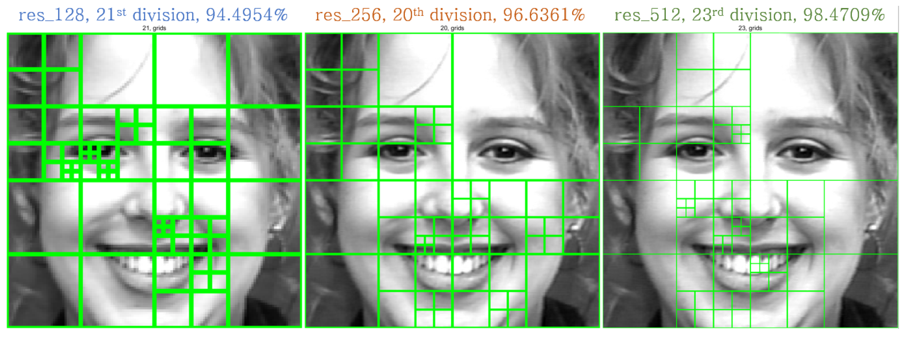
Depth	res_128	res_256	res_512
1	0	1	1
2	10	4	5
3	18	25	21
4	20	27	23
5	16	4	20

shows how the grids are distributed at each normalized resolution by depth. There are many high-depth grids distributed around the eyes, nose, and mouth, which clearly show facial expressions. Low-depth grids are distributed in the areas of the forehead, chin, and ear, which do not show facial expressions clearly.

As shown in Table 3, higher normalized resolutions result in a higher number of higher depth grids. This is interpreted as an improvement in overall classification accuracy caused by the improved resolution resulting in more information being obtained from higher depth grids.

4.3. Result of Feature Reduction

In addition to improving classification accuracy, FER using Grid Map also has the advantage of reducing the number of features required for the same accuracy. Figure 17 illustrates the cell distribution of two methods with similar classification accuracy. The left image shows the distribution of the HOG-ECOC classifier without adaptive feature extraction, and the right image shows the distribution of Grid Map.

In Figure 17, the Grid Map shows more efficient cell distribution and shows 0.39% higher classification accuracy even with fewer bins.

Table 4. Reduction rate of bin number and processing speed through Grid Map.

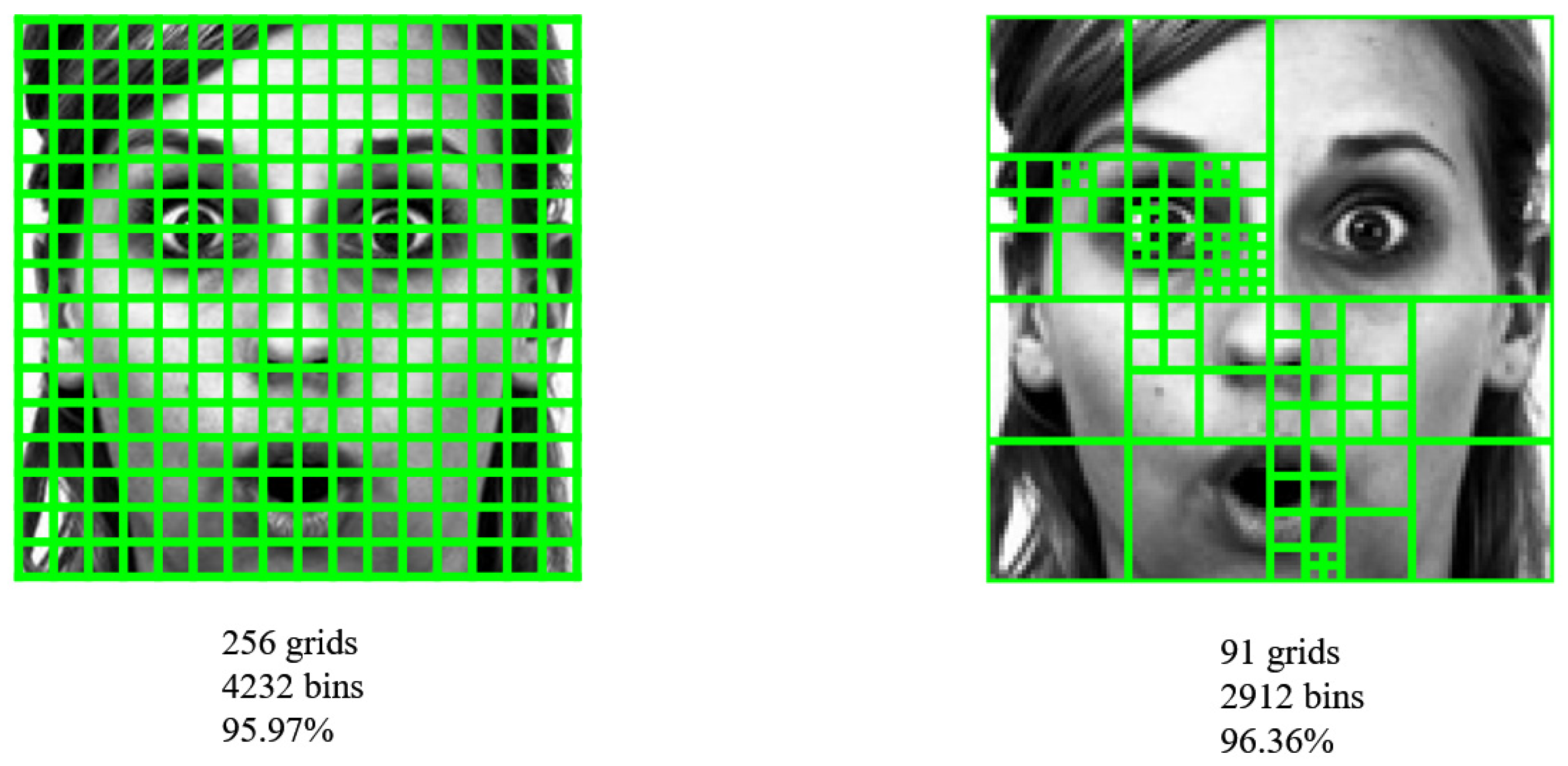
Method	Bins	Total Time (s)	Classifying an Image (ms)
Basic	4232	196.770	0.0602
Proposed	2912	130.520	0.0399
Ratio to basic (%)	68.81	66.33	66.28

shows the result of 1000 repeated experiments under the condition used to obtain Figure 17. classifying one image by random selection among 3105 images from the merged database.

Table 4 presents the computational costs for the basic and proposed methods. The total time (s) and time taken to classify an image (ms) correspond to all the computations for the classifications performed using a single thread of an Intel Core i7-8750H 2.3 GHz processor. Even though the proposed method involves more processes, it incurs a lower computational cost. This Grid Map is the optimal state of the merged database. The classification accuracy according to bin number is compared in

Table 5. Classification accuracy according to basic method and number of bins in Grid Map.

Basic Method			Proposed
Cell Size	Bins	Accuracy (%)	Bins	Accuracy (%)
32	145	78.20	128	57.91
30	174	79.36	128	57.91
28	212	81.26	224	76.04
26	259	80.23	224	77.04
24	321	88.05	320	82.87
22	402	86.38	416	87.09
20	512	91.95	512	91.34
18	664	93.27	704	93.11
16	882	94.81	896	94.33
14	1208	95.14	1184	95.10
12	1721	95.33	1760	95.72
10	2592	95.39	2624	96.14
8	4232	95.97	2816	96.04
6	7854	95.75	2912	96.36
4	18432	95.62	...	…
2	76832	94.98	3392	96.10

.

In Table 5, because the number of bins cannot be accurately compared with the basic method due to the algorithm, rows are arranged based on having a similar number of bins. If the cell size is smaller than 10 × 10, the number of bins in basic method increases exponentially and the accuracy improvement decreases after cell size 8 × 8. According to these results, Grid Map can classify facial expressions in 66.33% of the time required by the basic method under certain conditions.

The proposed method was able to classify the facial expressions more accurately with fewer features. In the adaptive feature extraction process, applying padding and increasing the database resolution to 512 × 512 improved classification accuracy by optimizing the Grid Map. For comparison, we collected experimental results using the CK+ database results from other papers discussing modified FER, as listed in

Table 6. Comparison of the proposed algorithm and other studies. SVM: support vector machine.

Method	Validation	Accuracy (%)
		Binary	Six Classes	Seven Classes
DCNN + SVM [23]	LOSO		97.08	96.02
HOG + SVM [24]	LOSO		96.40
BDBN [25]	8-fold	96.70
AUDN [4]	10-fold		95.78
Lopes et al. [5]	10-fold	98.92	96.76	95.75
LBP + SVM [26]	10-fold		95.10	91.40
Li et al. [27]	10-fold		98.18	97.38
Pu et al. [28]	10-fold			96.38
Zeng et al. [29]	10-fold			95.79
Proposed	10-fold			98.47

.

Table 6 shows that the proposed method has the highest classification accuracy when classifying seven classes. The classification accuracy of the proposed method for six classes was omitted but would be expected to be higher following the trend of existing results having higher accuracy for six classes than for seven. DCNN: Deep Convolutional Neural Network. BDBN: Boosted Deep Belief Network. AUDN: Action Unit-inspired Deep Network.

5. Discussion

The assumption of frontal face information being given with a few distortions is a limitation of this research. Because the images in the database used are not ideal fronts, the classification accuracy may have been diminished. In experimental results in Section 4, an optimal Grid Map that was quite close to assumption was derived as shown in the below figure. However, this Grid Map is not right and left symmetrical because it excludes the right and left symmetry of the actor’s expression. If this difference was not important, opposing girds would not been divided as in our assumption. However, in the optimal Grid Map, it can be inferred that the difference in left and right information may affect classification accuracy. Several other transformed images in the database have already been used for training. Figure 18 shows two examples of such images in the CK+ database.

The camera that captured the image on the left was rotated around the Z axis, and the camera that captured the image on the right was angled towards the actor from the bottom right. These images may affect the classification accuracy of the proposed method. Future study should include an additional pre-processing stage to consider changes in facial expression using the method proposed in this paper, with experimental results for comparison. Moreover, further validation is required in future research. Additional experimental results are also needed regarding the application of our proposed reinforcement learning to a study of classification accuracy improvement using a modified binary tree SVM by Lopes et al. [5] to classify neutral and other six expressions.

6. Conclusions

In this paper, we propose a modified ECOC-SVM classifier which is combined with reinforcement learning to improve its classification accuracy. To optimize training, the input image size is normalized according to the cascade rules of a pre-processing detector, and the regional weights are given by the adaptive cell size dividing each region of the image by bounding grids. HOG-ECOC was selected as the classification method through experiments for optimal feature and classifier selection, and it was then used as the reward value in Q-learning for optimizing Grid Map using 10-fold cross-validation. The proposed idea was formulated into a decision process and solved using Q-learning. Experimental results show 96.36% classification accuracy in the combined database and 98.47% in CK+. Comparing with the basic method at similar accuracy, the proposed method required only 68.81% of the features and 66.33% of the processing time.

References

- Michel, P.; El Kaliouby, R. Real time facial expression recognition in video using support vector machines. In Proceedings of the 5th International Conference on Multimodal interfaces, Vancouver, BC, Canada, 5–7 November 2003. [Google Scholar]
- Smola, A.J.; Schölkopf, B. A tutorial on support vector regression. Stat. Comput. 2004, 14, 199–222. [Google Scholar] [CrossRef]
- Huang, Y.; Chen, F.; Lv, S.; Wang, X. Facial Expression Recognition: A Survey. Symmetry 2019, 11, 1189. [Google Scholar] [CrossRef]
- Liu, M.; Li, S.; Shan, S.; Chen, X. Au-inspired deep networks for facial expression feature learning. Neurocomputing 2015, 159, 126–136. [Google Scholar] [CrossRef]
- Lopes, A.T.; de Aguiar, E.; De Souza, A.F.; Oliveira-Santos, T. Facial expression recognition with convolutional neural networks: Coping with few data and the training sample order. Pattern Recognit. 2015, 61, 610–628. [Google Scholar] [CrossRef]
- Yang, H.; Zhang, Z.; Yin, L. Identity-adaptive facial expression recognition through expression regeneration using conditional generative adversarial networks. In Proceedings of the 2018 13th IEEE International Conference on Automatic Face & Gesture Recognition, Xi’an, China, 15–19 May 2018; pp. 294–301. [Google Scholar]
- Zhang, Z.; Luo, P.; Loy, C.C.; Tang, X. Facial landmark detection by deep multi-task learning. In European Conference on Computer Vision, Proceedings of the ECCV 2014, Zurich, Switzerland, 6–12 September 2014; Springer: Cham, Switzerland, 2014. [Google Scholar]
- Tian, Y.-I.; Kanade, T.; Cohn, J.F. Recognizing action units for facial expression analysis. IEEE Trans. Panalysis Mach. Intell. 2001, 23, 97–115. [Google Scholar] [CrossRef] [PubMed]
- Dalal, N.; Triggs, B. Histograms of Oriented Gradients for Human Detection. In Proceedings of the International Conference on Computer Vision & Pattern Recognition (CVPR ’05), San Diego, CA, USA, 20–25 June 2005; pp. 886–893. [Google Scholar]
- Dietterich, T.G.; Bakiri, G. Solving multiclass learning problems via error-correcting output codes. J. Artif. Intell. Res. 1994, 2, 263–286. [Google Scholar] [CrossRef]
- Fei, B.; Liu, J. Binary tree of SVM: A new fast multiclass training and classification algorithm. IEEE Trans. Neural Netw. 2006, 17, 696–704. [Google Scholar] [CrossRef] [PubMed]
- Übeyli, E.D. ECG beats classification using multiclass support vector machines with error correcting output codes. Digit. Signal Process. 2007, 17, 675–684. [Google Scholar] [CrossRef]
- Bellman, R. A Markovian decision process. J. Math. Mech. 1957, 6, 679–684. [Google Scholar] [CrossRef]
- Howard, R.A. Dynamic Programming and Markov Processe; John Wiley: New York, NY, USA, 1960. [Google Scholar]
- Shapley, L.S. Stochastic games. Proc. Natl. Acad. Sci. 1953, 39, 1095–1100. [Google Scholar] [CrossRef] [PubMed]
- Watkins, C.J.; Dayan, P. Q-learning. Mach. Learn. 1992, 8, 279–292. [Google Scholar] [CrossRef]
- Lyons, M.J.; Akamatsu, S.; Kamachi, M.; Gyoba, J.; Budynek, J. The Japanese female facial expression (JAFFE) database. In Proceedings of the third International Conference on Automatic Face and Gesture Recognition, Nara, Japan, 14–16 April 1998. [Google Scholar]
- Lundqvist, D.; Flykt, A.; Öhman, A. The Karolinska directed emotional faces (KDEF). CD ROM Dep. Clin. Neurosci. Psychol. Sect. Karolinska Inst. 1998, 91, 2. [Google Scholar]
- Aifanti, N.; Papachristou, C.; Delopoulos, A. The MUG facial expression database. In Proceedings of the 11th International Workshop on Image Analysis for Multimedia Interactive Services WIAMIS 10, Desenzano del Garda, Italy, 12–14 April 2010. [Google Scholar]
- Olszanowski, M.; Pochwatko, G.; Kuklinski, K.; Scibor-Rylski, M.; Lewinski, P.; Ohme, R.K. Warsaw set of emotional facial expression pictures: A validation study of facial display photographs. Front. Psychol. 2015, 5, 1516. [Google Scholar] [CrossRef] [PubMed]
- Lucey, P.; Cohn, J.F.; Kanade, T.; Saragih, J.; Ambadar, Z.; Matthews, I. The extended cohn-kanade dataset (ck+): A complete dataset for action unit and emotion-specified expression. In Proceedings of the 2010 IEEE Computer Society Conference on Computer Vision and Pattern Recognition-Workshops, San Francisco, CA, USA, 13–18 June 2010. [Google Scholar]
- Viola, P.; Jones, M. Rapid object detection using a boosted cascade of simple features. In Proceedings of the 2001 IEEE Computer Society Conference on Computer Vision and Pattern Recognition (CVPR 2001), Kauai, HI, USA, 8–14 December 2001; pp. 511–518. [Google Scholar]
- Mayya, V.; Pai, R.M.; Pai, M.M. Automatic facial expression recognition using DCNN. Procedia Comput. Sci. 2016, 93, 453–461. [Google Scholar] [CrossRef]
- Matthews, I.; Baker, S. Active appearance models revisited. Int. J. Comput. Vis. 2004, 60, 135–164. [Google Scholar] [CrossRef]
- Liu, P.; Han, S.; Meng, Z.; Tong, Y. Facial expression recognition via a boosted deep belief network. In Proceedings of the IEEE Conference on Computer Vision and Pattern Recognition, Columbus, GA, USA, 20–23 June 2014. [Google Scholar]
- Shan, C.; Gong, S.; McOwan, P.W. Facial expression recognition based on local binary patterns: A comprehensive study. Image Vis. Comput. 2009, 27, 803–816. [Google Scholar] [CrossRef]
- Li, K.; Jin, Y.; Akram, M.W.; Han, R.; Chen, J. Facial expression recognition with convolutional neural networks via a new face cropping and rotation strategy. Vis. Comput. 2019, 36, 391–404. [Google Scholar] [CrossRef]
- Pu, X.; Fan, K.; Chen, X.; Ji, L.; Zhou, Z. Facial expression recognition from image sequences using twofold random forest classifier. Neurocomputing 2015, 168, 1173–1180. [Google Scholar] [CrossRef]
- Zeng, N.; Zhang, H.; Song, B.; Liu, W.; Li, Y.; Dobaie, A.M. Facial expression recognition via learning deep sparse autoencoders. Neurocomputing 2018, 273, 643–649. [Google Scholar] [CrossRef]