Implementing CCTV-Based Attendance Taking Support System Using Deep Face Recognition: A Case Study at FPT Polytechnic College

 , ,
, ,  and
and
Abstract
1. Introduction
1.1. Problem and Motivation
1.2. Related Works
1.3. Problems of Face Recognition in Attendance Taking System Using CCTV
1.4. Contribution of This Paper
2. Proposed System
2.1. Job Master
2.2. Job Workers
2.3. Face Recognition Building Block
2.3.1. Data Sampling
2.3.2. Region of Interest
2.3.3. Frame Processing and Responding Time
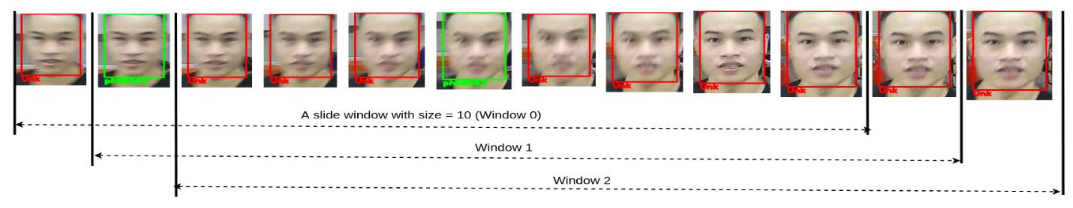
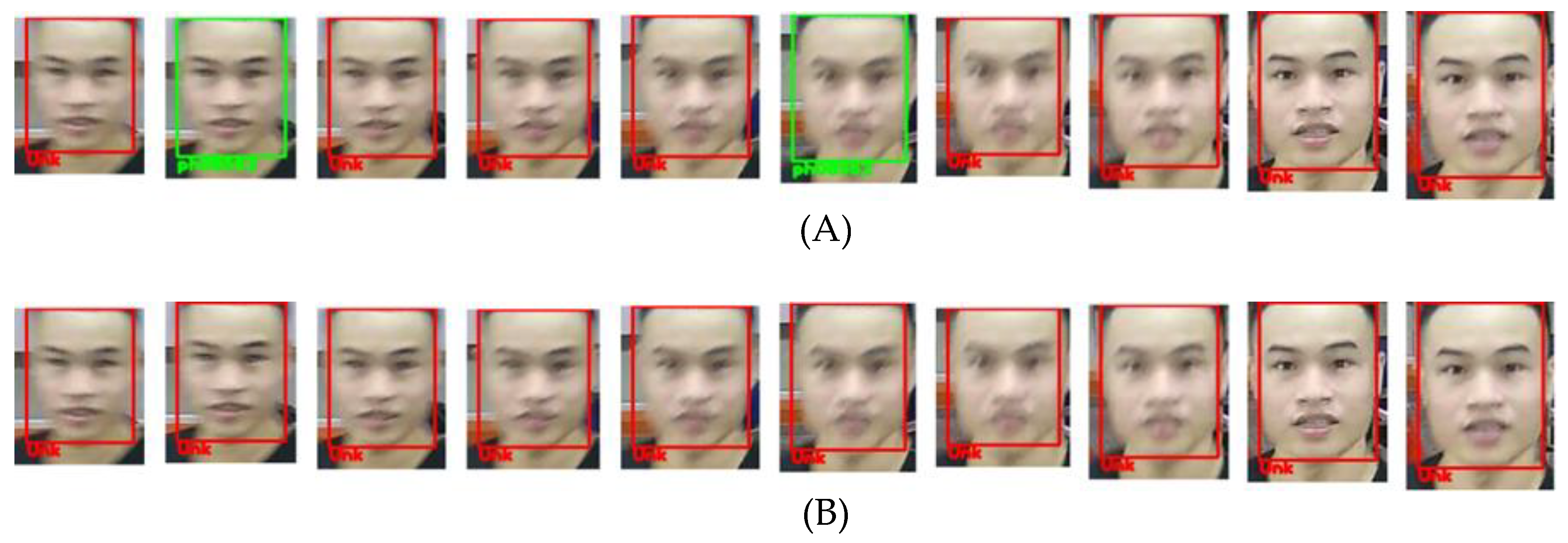
2.3.4. Summarization Algorithm
3. Experiment and Result
3.1. Experiment
3.2. System Accuracy
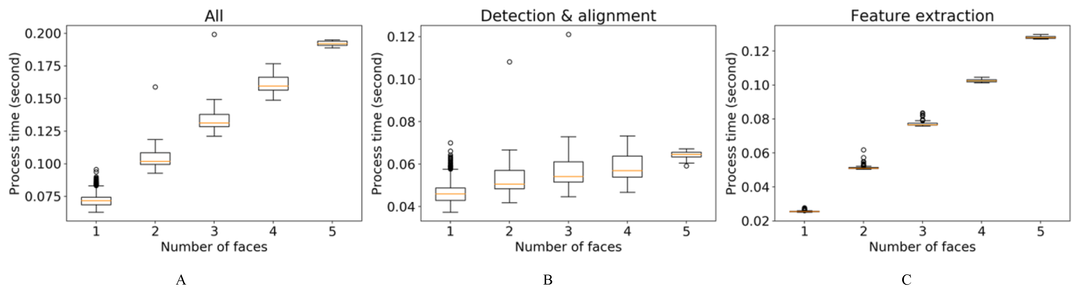
3.3. System Processing Time
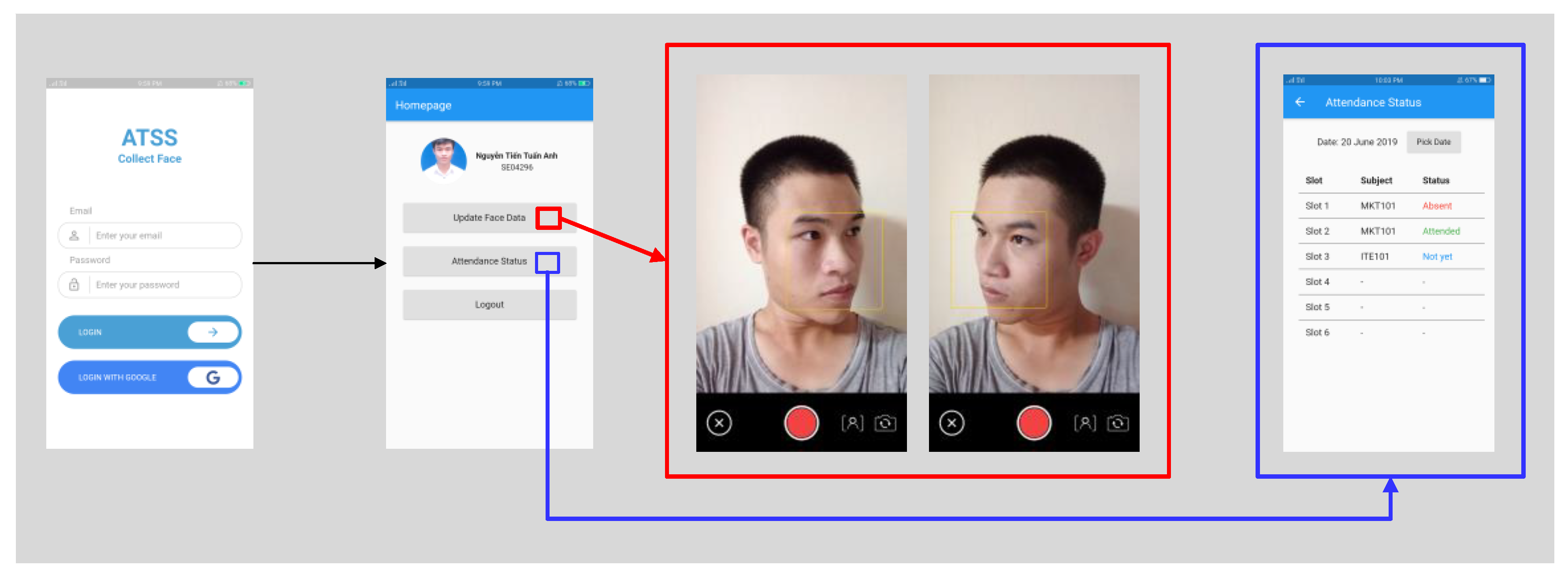
3.4. Application
4. Conclusions
Author Contributions
Funding
Conflicts of Interest
References
- Minaee, S.; Abdolrashidi, A.; Su, H.; Bennamoun, M.; Zhang, D. Biometric recognition using deep learning: A survey. arXiv 2019, arXiv:1912.00271. [Google Scholar]
- Son, N.T.; Chi, L.P.; Lam, P.T.; Van Dinh, T. Combination of facial recognition and interaction with academic portal in automatic attendance system. In Proceedings of the 2019 8th International Conference on Software and Computer Applications (ICSCA ’19). ACM, New York, NY, USA, 19–21 February 2019; pp. 299–305. [Google Scholar] [CrossRef]
- Shoba, D.; Sumathi, C.P. A Survey on Various Approaches to Fingerprint Matching for Personal Verification and Identification. International Journal of Computer Science & Engineering Survey (IJCSES), 7 August 2016; Volume 7, No. 4. [Google Scholar] [CrossRef]
- Balaban, S. Deep learning and face recognition: The state of the art. arXiv 2015, arXiv:1902.03524. [Google Scholar]
- Yu, H.; Luo, Z.; Tang, Y. Transfer learning for face identification with deep face model. In Proceedings of the 2016 7th International Conference on Cloud Computing and Big Data (CCBD), Macau, China, 16–18 November 2016. [Google Scholar] [CrossRef]
- Wang, M.; Deng, W. Deep face recognition: A survey. arXiv 2019, arXiv:1804.06655v8. [Google Scholar]
- Deng, J.; Guo, J.; Zafeiriou, S. Arcface: Additive angular margin loss for deep face recognition. arXiv 2018, arXiv:1801.07698. [Google Scholar]
- Liu, W.; Wen, Y.; Yu, Z.; Li, M.; Raj, B.; Song, L. SphereFace: Deep hypersphere embedding for face recognition. In Proceedings of the 2017 IEEE Conference on Computer Vision and Pattern Recognition (CVPR), Honolulu, HI, USA, 21–26 July 2017. [Google Scholar] [CrossRef]
- Schrof, F.; Kalenichenko, D.; Philbin, J. FaceNet: A unified embedding for face recognition and clustering. arXiv 2015, arXiv:1503.03832V3. [Google Scholar]
- Wang, H.; Wang, Y.; Zhou, Z.; Ji, X.; Gong, D.; Zhou, J.; Liu, W. CosFace: Large margin cosine loss for deep face recognition. In Proceedings of the 2018 IEEE/CVF Conference on Computer Vision and Pattern Recognition, Long Beach, CA, USA, 16–20 June 2018. [Google Scholar] [CrossRef]
- Ranjan, R.; Sankaranarayanan, S.; Bansal, A.; Bodla, N.; Chen, J.C.; Patel, V.M.; Castillo, C.D.; Chellappa, R. Deep learning for understanding faces: Machines may be just as good, or better, than humans. IEEE Signal Process. Mag. 2018, 35, 66–83. [Google Scholar] [CrossRef]
- Zhang, K.; Zhang, Z.; Li, Z.; Qiao, Y. Joint face detection and alignment using multitask cascaded convolutional networks. IEEE Signal Process. Lett. 2016, 23, 1499–1503. [Google Scholar] [CrossRef]
- Wang, H.; Li, Z.; Ji, X.; Wang, Y. Face R-CNN. arXiv 2017, arXiv:1706.01061. [Google Scholar]
- Farfade, S.S.; Saberian, M.; Li, L.-J. Multi-view face detection using deep convolutional neural networks. arXiv 2015, arXiv:1502.02766. [Google Scholar]
- Feng, Z.-H.; Kittler, J.; Awais, M.; Huber, P.; Wu, X.-J. Face detection, bounding box aggregation and pose estimation for robust facial landmark localisation in the wild. In Proceedings of the 2017 IEEE Conference on Computer Vision and pattern Recognition Workshops, (CVPRW), Honolulu, HI, USA, 21–26 July 2017. [Google Scholar] [CrossRef]
- Sagonas, C.; Antonakos, E.; Tzimiropoulos, G.; Zafeiriou, S.; Pantic, M. 300 faces in-the-wild challenge: Database and results. Image Vis. Comput. 2016, 47, 3–18, Special Issue on Facial Landmark Localisation “In-The-Wild”. [Google Scholar] [CrossRef]
- Brinkmann, R. The Art and Science of Digital Compositing; Morgan Kaufmann: Burlington, MA, USA, 1999; p. 184. ISBN 978-0-12-133960-9. [Google Scholar]
- Han, J.; Kamber, M.; Pei, J. Data Mining: Concepts and Techniques, 3rd ed.; Morgan Kaufmann Publishers Inc.: San Francisco, CA, USA, 2011. [Google Scholar]
- Course Syllabus EBIO 6300: Phylogenetic Comparative Methods-Fall 2013. Available online: https://www.colorado.edu/smithlab/sites/default/files/attached-files/EBIO6300_PCMsSyllabus.pdf (accessed on 1 June 2019).
- Space and Naval Warfare Systems Center Atlantic. CCTV Technology Handbook; System Assessment and Validation for Emergency Responders (SAVER), 2013.
- Zhou, Y.; Liu, D.; Huang, T. Survey of face detection on low-quality images. In Proceedings of the 2018 13th IEEE International Conference on Automatic Face & Gesture Recognition (FG 2018), Xi’an, China, 15–19 May 2018. [Google Scholar] [CrossRef]
- Masi, I.; Wu, Y.; Hassner, T.; Natarajan, P. Deep face recognition: A survey. In Proceedings of the 2018 31st SIBGRAPI Conference on Graphics, Patterns and Images (SIBGRAPI), Foz do Iguaçu, Brazil, 29 October–1 November 2018. [Google Scholar] [CrossRef]
- Ngoc Anh, B.; Tung Son, N.; Truong Lam, P.; Phuong Chi, L.; Huu Tuan, N.; Cong Dat, N.; Huu Trung, N.; Umar Aftab, M.; Van Dinh, T. A computer-vision based application for student behavior monitoring in classroom. Appl. Sci. 2019, 9, 4729. [Google Scholar] [CrossRef]
- Li, J.; Zhang, D.; Zhang, S. The application and research on master-slave station distributed integration business architecture. In Proceedings of the 2016 IEEE Advanced Information Management, Communicates, Electronic and Automation Control Conference (IMCEC), Xi’an, China, 3–5 October 2016. [Google Scholar] [CrossRef]
- Wang, X.; Wang, K.; Lian, S. A survey on face data augmentation. arXiv 2019, arXiv:1904.11685. [Google Scholar]
- Ruiz, N.; Chong, E.; Rehg, J.M. Fine-grained head pose estimation without keypoints. In Proceedings of the IEEE Conference on Computer Vision and Pattern Recognition (CVPR) Workshops, Salt Lake City, UT, USA, 18–22 June 2018; pp. 2074–2083. [Google Scholar]
- Murphy, K.P. Machine Learning: A Probabilistic Perspective, 1st ed.; Adaptive Computation and Machine Learning series; MIT Press: Cambridge, MA, USA, 2012. [Google Scholar]
- Yilmaz, A.; Javed, O.; Shah, M. Object tracking: A survey. ACM Comput. Surv. 2006, 38. [Google Scholar] [CrossRef]
- Van der Maaten, L.; Geoffrey, H. Visualizing data using t-SNE. J. Mach. Learn. Res. 2008, 9, 2579–2605. [Google Scholar]
- Wang, J.; Chen, Q.; Chen, Y. RBF kernel based support vector machine with universal approximation and its application. In Advances in Neural Networks—ISNN 2004; Yin, F.L., Wang, J., Guo, C., Eds.; Lecture Notes in Computer Science; Springer: Berlin/Heidelberg, Germany, 2004; Volume 3173, ISNN 2004. [Google Scholar]
- Hechenbichler, K.; Schliep, K. Weighted K-Nearest-Neighbor Techniques and Ordinal Classification; Discussion paper 399; SFB 386; Ludwig-Maximilians University: Munich, Germany, 2004; Available online: http://www.stat.uni-muenchen.de/sfb386/papers/dsp/paper399.ps (accessed on 25 June 2019).
- Zhou, S.; Xiao, S. 3D face recognition: A survey. Hum. Cent. Comput. Inf. Sci. 2018, 8, 35. [Google Scholar] [CrossRef]
- Marcolin, F.; Violante, M.G.; Sandro, M.O.O.S.; Vezzetti, E.; Tornincasa, S.; Dagnes, N.; Speranza, D. Three-dimensional face analysis via new geometrical descriptors. In Lecture Notes in Mechanical Engineering; Springer: Cham, Switzerland, 2017; pp. 747–756. [Google Scholar] [CrossRef]
- Widanagamaachchi, W.N.; Dharmaratne, A.T. 3D Face Reconstruction from 2D Images. In Proceedings of the 2008 Digital Image Computing: Techniques and Applications, Canberra, ACT, Australia, 1–3 December 2008; pp. 365–371. [Google Scholar] [CrossRef]
- Jiang, L.; Zhang, J.; Deng, B.; Li, H.; Liu, L. 3D face reconstruction with geometry details from a single image. IEEE Trans. Image Process. 2018, 27, 4756–4770. [Google Scholar] [CrossRef] [PubMed]


| Classifiers | Linear SVM | RBF SVM | NB | WKNN | Mean | |
|---|---|---|---|---|---|---|
| Descriptor | ||||||
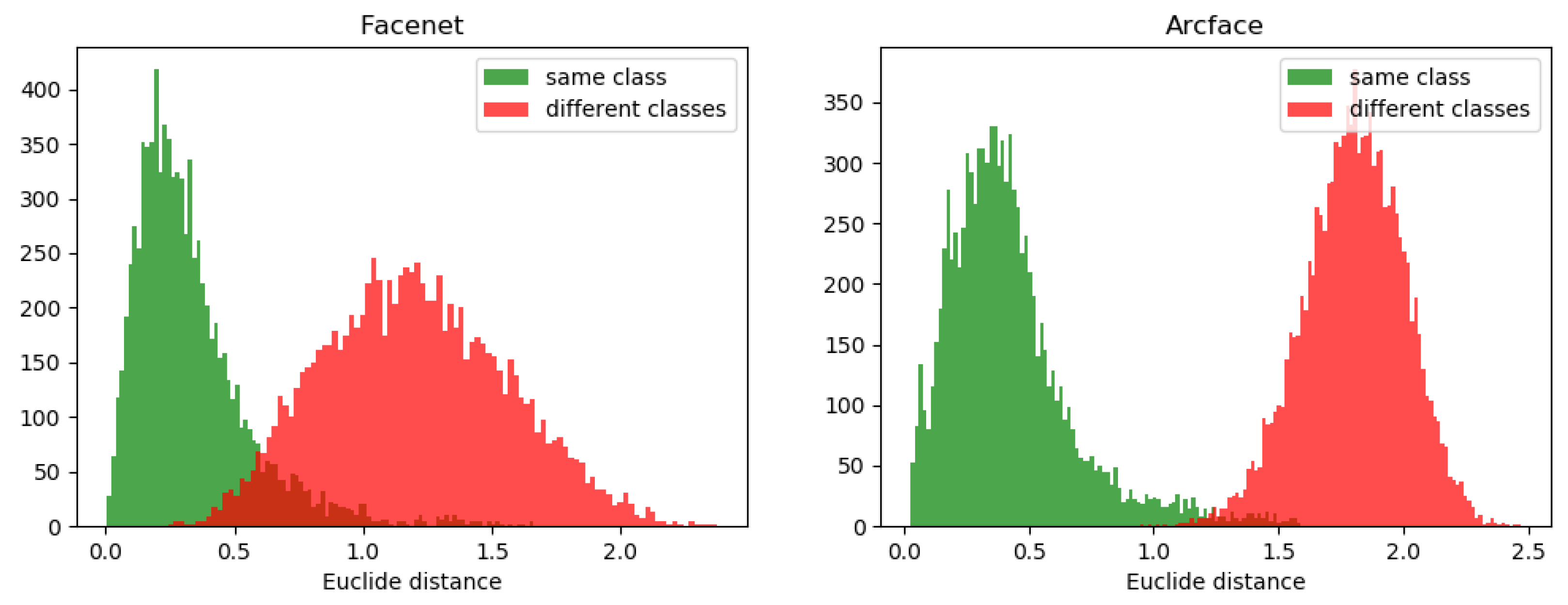
| FaceNet | 0.643 | 0.638 | 0.6 | 0.652 | 0.633 | |
| ArcFace | 0.886 | 0.803 | 0.75 | 0.913 | 0.83 | |
© 2020 by the authors. Licensee MDPI, Basel, Switzerland. This article is an open access article distributed under the terms and conditions of the Creative Commons Attribution (CC BY) license (http://creativecommons.org/licenses/by/4.0/).
Share and Cite
Son, N.T.; Anh, B.N.; Ban, T.Q.; Chi, L.P.; Chien, B.D.; Hoa, D.X.; Thanh, L.V.; Huy, T.Q.; Duy, L.D.; Hassan Raza Khan, M. Implementing CCTV-Based Attendance Taking Support System Using Deep Face Recognition: A Case Study at FPT Polytechnic College. Symmetry 2020, 12, 307. https://doi.org/10.3390/sym12020307
Son NT, Anh BN, Ban TQ, Chi LP, Chien BD, Hoa DX, Thanh LV, Huy TQ, Duy LD, Hassan Raza Khan M. Implementing CCTV-Based Attendance Taking Support System Using Deep Face Recognition: A Case Study at FPT Polytechnic College. Symmetry. 2020; 12(2):307. https://doi.org/10.3390/sym12020307
Chicago/Turabian StyleSon, Ngo Tung, Bui Ngoc Anh, Tran Quy Ban, Le Phuong Chi, Bui Dinh Chien, Duong Xuan Hoa, Le Van Thanh, Tran Quang Huy, Le Dinh Duy, and Muhammad Hassan Raza Khan. 2020. "Implementing CCTV-Based Attendance Taking Support System Using Deep Face Recognition: A Case Study at FPT Polytechnic College" Symmetry 12, no. 2: 307. https://doi.org/10.3390/sym12020307
APA StyleSon, N. T., Anh, B. N., Ban, T. Q., Chi, L. P., Chien, B. D., Hoa, D. X., Thanh, L. V., Huy, T. Q., Duy, L. D., & Hassan Raza Khan, M. (2020). Implementing CCTV-Based Attendance Taking Support System Using Deep Face Recognition: A Case Study at FPT Polytechnic College. Symmetry, 12(2), 307. https://doi.org/10.3390/sym12020307