Abstract
Face recognition (FR) has received considerable attention in the field of security, especially in the use of closed-circuit television (CCTV) cameras in security monitoring. Although significant advances in the field of computer vision are made, advanced face recognition systems provide satisfactory performance only in controlled conditions. They deteriorate significantly in the face of real-world scenarios such as lighting conditions, motion blur, camera resolution, etc. This article shows how we design, implement, and conduct the empirical comparisons of machine learning open libraries in building attendance taking (AT) support systems using indoor security cameras called ATSS. Our trial system was deployed to record the appearances of 120 students in five classes who study on the third floor of FPT Polytechnic College building. Our design allows for flexible system scaling, and it is not only usable for a school but a generic attendance system with CCTV. The measurement results show that the accuracy is suitable for many different environments.
1. Introduction
1.1. Problem and Motivation
Every day, the CCTV system operates to monitor the inside of a building for security. The system’s resources allow developers to build computer vision-based applications to integrate with CCTV. Face recognition (FR) is an excellent biometric technique for identity authentication [1]. It is possible to apply FR technology for automatic attendance taking at schools. There are several benefits from attendance considering using the existing camera system, such as save time and effort, provide striking evidence for quality assurance and human resource management tasks, avoid intermediary of infectious diseases [2]. The existing attendance taking system that uses fingerprint recognition is facing several challenges due to large intra-class variability and substantial inter-class similarity mentioned by Dyre and Sumathi [3]. Ngo et al. combined the data from the academic portal with different FR techniques for the task of taking attendance in the classroom [2]. The result shows that their system works smoothly. However, the investment costs for procurement, camera installation at the school, and a large number of video processing are expensive. This research describes the solution to apply deep FR technology to perform AT via the existing CCTV system, which takes advantage of the available resources better and more suitable for different situations. We used a case study at FPT Polytechnic college to illustrate our design. Figure 1 displays some photos captured from the real deployed system.
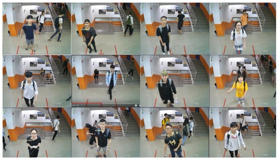
Figure 1.
Real installation of the attendance taking support system (ATSS) at the third floor at FPT Polytechnic School.
1.2. Related Works
Recently, deep learning techniques have made many significant achievements in FR, such as deep convolutional neural networks [4] use a cascade of multiple layers of processing units for feature extraction. They learn various levels of representations that correspond to different levels of abstraction. These techniques are called deep FR. The evolution of the FR is around network architectures and loss functions. Deep face model trained on the large dataset. We often lack resources to learn a complex model with minimal training samples for a specific face recognition task. Therefore, using the pre-trained model as transfer learning is usually applied [5]. Wang and Deng reviewed many model techniques [6] such as ArcFace [7] proposed a new loss function, additive angular margin to learn highly discriminative features for robust face recognition. SphereFace [8] used ResNet 64 architecture and angular softmax loss to learn discriminative face features with the angular margin. Another face embedding is FaceNet [9] that uses a new triplet loss function and a large private dataset to train a GoogleNet. Cosface [10] introduced their loss function based on a cosine margin term to maximize the decision margin in the angular space. They are some of the famous representatives along with other Deep FR works that are recently published. The surveys show that most of the review models gain high achievements, with more than 98% to almost 100% accuracy on the tested datasets.
Ranjan et al. summarized FR’s component consists of three modules usually used in face recognition [11], as shown in Figure 2: (A) The face detector: applied to localize faces in images or videos. A powerful face detector can provide different pose, illumination, and scale. It returns a bounding box of the face that minimizes the background [12,13,14,15]. (B) Facial landmarks extractor: detects the facial landmarks such as eye centers, nose tip, and mouth corners. These points are essential to align the faces to normalized canonical coordinates. Typically, the deep face detector also goes with landmarks points [12,13,14,15,16]. Landmarks make it easy to detect face poses and some other processes such as face alignment. (C) Feature descriptor: that encodes the identity information secured from the aligned face. The similarity scores are then obtained between them that are used in face identification [7,8,9,17]. The purpose of this is to enhance the separation between the face data of different individuals, and through that improve the ability to classify and cluster. The universal approaches of classification algorithms, one-versus-all, all-versus-all (alternative of one-all-all) can all be severe with a large number of labels [18]. As mentioned in the previous section Ngo and colleagues proposed to narrow the scope of classification problems by using multiple classifiers, each of which will be used only for a specific group of students based on their class schedule [2]. Their contributions inspire our research.

Figure 2.
Illustration of three main components of the deep face system. (A) demonstrates the face detection from an image frame, (B) shows the landmarks points of the cropped faces, and (C) plot featured data in feature space archived by feature descriptor.
1.3. Problems of Face Recognition in Attendance Taking System Using CCTV
The picture seems simple when we think that we only need to use FR to determine if students are present. However, when we carried out our investigation, we faced some problems: (1) Required almost 100% accuracy: attendance usually affects students directly. Many schools also require attendance as part of the assessment process. See an example of the course syllabus for EBIO 6300 of the University of Colorado in semester fall-2013 [19]. At FPT polytechnic, the minimum attendance required is 80% (over 30 slots of studying). There are several strategies to solve the problem apart from the special technical efforts such as additional policy, system support, etc. (2) Constrained because of the environment: installed equipment is mainly used for security purposes instead of attendance taking [20]. The cameras are hung at the intersection in the corridor, such as the elevator hall, corridor corner. The AT must not generate any effects on the existing CCTV system. (3) Performance of the current methods in a real environment: even if the accuracy of ArcFace [7], the highest archive algorithm mentioned in [6] is up to 99.83% on MS-Celeb-1M test set. Algorithms almost work well in an ideal environment, which may not be satisfied in the real settings because of the effect of motion, camera resolution [21], light conditions. The attendance taking task may not require to respond in runtime; however, the delay should be as short as possible, or it is feasible to do this by increasing the processing capacity of the system. Meanwhile, most of the high accuracy libraries implement the state-of-the-art in FR asked for high processing time. (4) Ability to integrate with existing systems: attendance taking system has a significant influence on the way the performance of attendees is measured. System integration relates to user habits and operating experience. Therefore, they need to be able to leverage the available resources of existing information systems. Besides, these systems also bring other benefits to the attendance system.
1.4. Contribution of This Paper
The main contribution of this paper is to develop a complete algorithmic process that, at each step, has been studied and evaluated to find the appropriate processing method for an automatic attendance system using CCTV problems. The system consists of four major parts: the job master, job workers, a central database, and user interface applications. The job master plays the role of a navigator and controls the AI processing units, which relates to the issues of performance of the system, and are focused parts of this research.
The existing solution cannot solve the mentioned problems with AT using CCTV without adding some calibrations. In this paper, we describe the way to provide experiments, combine techniques, and to prepare some environment settings to tune our attendance taking system. Performance indicators, along with business requirements, are considered to indicate detailed recommendations on investment costs as well as the benefits for a particular system scale. Our system provides a guide that not only allows the construction of a specific attendance system but is a general method for the attendance system. Moreover, this architecture is workable for processing computer vision in real systems. Our design allows the expansion of processing units (plug-ins) to deal with the system at a larger scale. Combining with existing information systems plays a role in narrowing down the range of calculations and improving reliability. Our proposed summarization algorithm improved the accuracy of the methods used.
Several surveys summarize, and literature reviews the FR libraries [6,11,22]. In this study, we provide an empirical comparison of the latest FR libs as well as classification algorithms through our dataset in our real environment project. Ngo et al. also conducted a review on libraries, but the reviewed facial embedding libs were out of date [2]. The remainder of the paper is organized as follows: Section 2 describes the architectural design of the system. Section 3 shows the tested results, and brief conclusions are finally discussed in part 4.
2. Proposed System
The attendance system, called ATSS, connects to the CCTV system. ATSS operates dependently on the CCTV system but does not leave any effect on the existing system. Figure 3 depicts the general picture of the system. There are several components in the system: the media recorder, job master, job workers, central database, and user interface applications. The media recorder plays the role to record frames captured from the CCTV system for further processes. The job master constructs, schedules, and arranges tasks to job workers by using data leveraged from the academic portal. The processed data then stored in the central database are accessed by the user for reporting and manipulating data via the web application. The attendance data are also submitted to the academic portal. The system admin can configure all parameters. The architecture has many similarities with the system architecture of Bui et al. [23]. However, it allows the system to be more flexible in terms of processing; the system’s response is possible to configure to fit the computational resources. The next parts of this section provide a detailed description of the particular module.
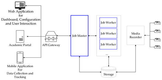
Figure 3.
ATSS system architecture.
2.1. Job Master
As a navigator of the system, the job master is responsible as the navigator of the data streams and process—the system runs according to the schedule data. The corresponding FR model is also loaded based on the list of students instead of constructing a significant model for identifying the whole students. The API Gateway allows APIs to communicate with existing systems. Class diagram represents the exchanged data structure between ATSS and the academic portal as shown in Figure 4. In the general problem, students are the attendees. The entities and relationships linked with the scheduling entity may need to be modified according to actual conditions. The system APIs are available with the building management system configured via the administrator’s web application, for example, synchronized list attendees, floors list, rooms list, and so on. The process of data synchronization allows the system to be compatible with existing systems, thus enhancing the adaptability.
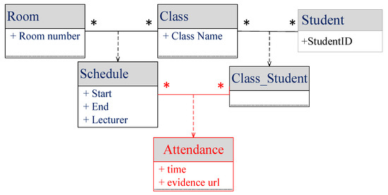
Figure 4.
Class diagram represents the data structure of exchanged data between the ATSS and the academic portal. Classes and relationships are described in black to represent the data that ATSS receives from the academic portal. The classes and relationships highlighted.
According to the performance of the models reviewed by [2] and [6], because of our limited computation resources, deep FR’s performance cannot be satisfied to perform run-time response. We group the archived frames and corresponding schedules into several jobs and push to a queue. Each of them dequeued to process by the job workers. Figure 5 demonstrates the process of dividing the archived frames into tasks. This process allows speeding up the calculation by adding more job workers. The job master acts as a workload balancer, which controls the works among the workers to avoid bottleneck and race conditions.
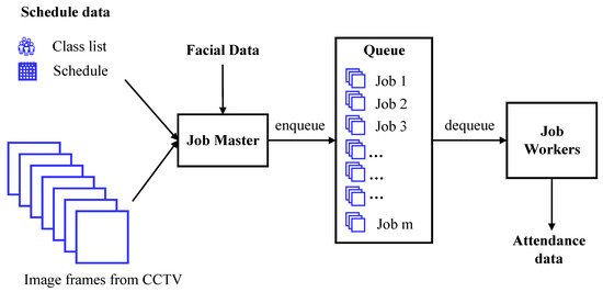
Figure 5.
Archived image frames from CCTV are divided into jobs and stores in the queue for next process.
2.2. Job Workers
Another module that plays an essential part in the architecture shown in Figure 3 is job worker. It performs the simple task of an FR problem. All descriptions of FR building blocks are available in this module (the detail of FR is already mentioned in Section 1). The video frames are processed directly in this module. All processes are in parallel through the arrangement of the job master. They are constructed based on master-slave architecture [24]. This architecture allows us to work efficiently with extensive data when deploying systems on a larger scale (hundreds of cameras). There are two tasks handled by the workers as shown in Figure 6: (1) Face identification: Photos of batches taken from the queue passed to the identification module. The system does not have to process the whole pixels of an image. The region of interest is cropped for the subsequent processing. Face and landmark detections are executed to retrieve bounding boxes of the faces as well as facial landmarks points. There are several techniques for face data augmentation reviewed by Wang et al. [25], such as face rotation, transformation… etc. However, we applied a compelling face-embedding technique for feature description based on our observation during the system development. We notice that face alignment brings efficiency. All cropped faces passed to vectorization for the classification task. The summarization algorithm (described in the section) was performed to make the final decision. (2) Data collection: Features are extracted from video faces collected by the mobile application, and then processed in frame processing component and stored as feature vectors in the database. This process does not require an almost real-time response, so a parallel processing architecture is not needed. To provide the front-end to collect the training dataset, we have built a mobile application to record the user’s face video. The user uses the front camera of the phone to record different angles of the face in the lowest resolution of 720 p, 30 fps. The average length of the trained videos is about 30 s. Videos are recorded by the data collector and then uploaded to the database server for further processing via a web service. Section 2.3 describes in detail how each handle of the FR building block is installed in job worker.
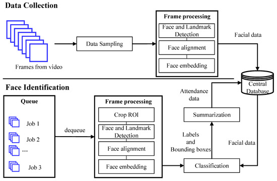
Figure 6.
Components of an Ai processing unit.
2.3. Face Recognition Building Block
In this section, we describe in detail how we configure for each system component. The description mainly lies around the modules that are the most effective, including data sampling, batch processing, the defining region of interest (ROI), frame processing, and summarization algorithm.
2.3.1. Data Sampling
We do not take all retrieved frames from uploaded videos by the data collector application to build a training dataset. Instead of doing so, on each video, we perform head pose detection using HopeNet [26] to detect exactly three face turning angles. In our experiment, the best value of three face turning angles is −0.3 rad, 0 rad, and 0.3 rad. After that, we perform face detection to extract three faces in each corner. We have nine faces evenly spread from the input video that is the number of training samples for each class. The facial embedding methods used are all pre-trained models with millions of face data, so images in normal conditions can be encoded under feature vectors that are separate from faces in other classes. Feature vectors are then extracted from the cropped faces to be stored in the facial database. Figure 7 illustrates an example of nine faces collected.
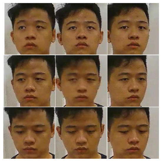
Figure 7.
Example of nine faces collected of a particular student.
2.3.2. Region of Interest
We found that FR only works well within a certain distance; the problem may relate to the camera resolution and motion blur effects in many types of CCTV. So we calculated the area to take attendance, which is a rectangle called attendance area, and asked for a rule to guide students to go through this area to record their presence. For specific identification, we propose a correction plan in each particular camera type based on the labeled data. We found that if the center of the data belongs to a specific label closest to the input sample, that is precisely the distance we find. In other words, if you sit on the chair to watch for some known-people to pass by, the range you see that person’s face clear the best is the region of interest (ROI). To do this, we used the similarity between the center of the group and the input sample. There are many types of similarity measures. However, because of the face embedding methods we choose, we decided to use the Euclidean distance. Different type of cameras provide different resolution, projection angle; depending on the particular environment, we need to perform calibration for each of them. The detail of the algorithm described is as follows:
Denote: are the training set of seven members in the project team. Where is the number of labelled images in the class and is the size of dimension space, depending on the face embedding methods we selected. We calculate the center of :
is the feature vector capture member when he stands meters away from the camera, his face turn directly to the camera. We compute the distance from to . Set is the mean of the particular distance to camera of the seven members. Figure 8 displays similarity degrees and the corresponding distance to camera.
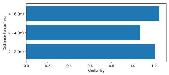
Figure 8.
Illustration of the similarity between the test faces and the mean of the training faces (Euclidean distance, the closer is better) corresponding to a particular range to camera.
The camera is hanging at the height of 2.8 m. The distance from the face to the camera is about 2 m to 4 m, which is the ideal distance for FR. In practice, we choose 2.5 m to 3.5 m. To speed up the processing, we set up so that three people can stand in horizontal line and still be able to check. We set the height of the attendance area as 100 cm (equivalent to 3-floor tiles). We then cropped the image to fit the size of five humans step in the attendance area. The area is called the region of interest (ROI) [17].
2.3.3. Frame Processing and Responding Time
The system only considers faces that appear in the ROI. Ngo et al. reviewed the face detection libraries. According to the results obtained from them, we use MTCNN [12] as a face and landmark detector. The faces are aligned based on five returned landmark points (left eye, right eye, nose, left corner mouth, and right corner mouth). We already consider some of the face embedding libraries mentioned in Wang and Deng’s survey [6] including: Arcface [7], Sphereface [8], Facenet [9], Cosface [10]. The main goal of these methods is to maximize face class separability by introducing a new loss function that is highly discriminative to features for face recognition. According to the survey. Although, Arcface showed the best results compared to other loss functions that are good with face recognition like triplet loss, intra-loss, and inter-loss. However, through initial empirical results, they all show adverse effects in the real environment (because of light condition, motion blur…) without our post-processing. We tested some different FR libraries and their output feature vectors with several machine learning algorithms including parametric and non-parametric, generative, and discriminative [27].
At FPT polytechnic, if the student is late for the first 15 min, or leave early before the last 15 min, he/she is counted as absent. Attendance usually takes place at this time. To increase flexibility in attendance as well as to avoid affecting the class, we define the AT process consist of two phases: check-in and check-out for this process. The check-in time starts 15 min earlier than the lesson and ends after the first 15 min. Likewise, for check-out at the end of class. Students present in front of the attendance taking area at the right time are considered as present. The AT may not strictly require runtime responding. However, it should get a response as fast as possible. In this situation, we set 2 min as the size of a job. We tried many different sizes; however, 2 min is the best-observed value because of the aspects of waiting time, processing time, and memory consumption.
2.3.4. Summarization Algorithm
Using pure FR to classify input faces generates a mess because of the motion blur and the deflection angle of the faces to the camera. Each human goes through the ROI, creating dozens of frames. Some of the samples are classified correctly, but some others are not. Our idea is to track every face in ROI as object tracking [28], the class assigned to a particular sample will mostly be the final decision. However, this number of identifiers must be more than one threshold, which we have set is ten frames. The summarize algorithm consists two main steps as follows:
Step 1—connected bounding box detection: Each bounding box have four attributes: . Any two of the bounding boxes are considered connected if they are at most two frames away from each other and their ratio of intersection is greater than as we found in the experiment, or they are connected with a common bounding box. A connected component of bounding boxes contain all the bounding boxes connected pairwise. They are the movement of a face in a video. Figure 9 illustrates the connected bounding boxes.

Figure 9.
Example of connected bounding boxes.
Step 2—final decision: For each connected component, we use a sliding window algorithm with window size and slide to the right to determine the range for labeling (see Figure 10). For each window, we label by using the time that label appear and the predicted ratio is used to determine whether that label can label all the boxes in that window or not. As in the experiment, the best value for this ratio is 0.6. If no label satisfies the condition, all boxes in that window will be labeled “Unknown”.

Figure 10.
Example of a sliding window.
As shown in Figure 11, all wrong labels are labeled again, and in the next window, we use the old (not updated) label and continue labeling. This function will reduce the rate of the wrong detection in our system.
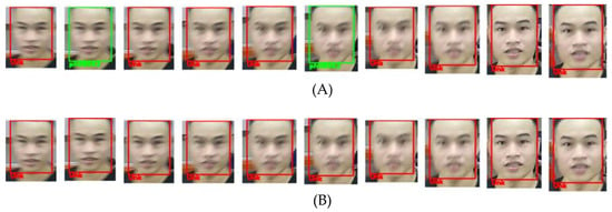
Figure 11.
Example of the output of the summarization algorithm. (A) Illustrates the pure classification results. (B) The most frequent label (class) assigned to the whole boxes appear in the window.
3. Experiment and Result
3.1. Experiment
We used the pre-trained models to build the system. Therefore, in order to carry out the evaluation of appropriate models, we use the facial data of 120 students as the training data (as described in Section 2.2 and Section 3.1, there are nine facial images for each student). Test data were recorded in two sessions, with 7490 labeled images in attendant time. We manually labeled each face that appears in the ROI in videos. Figure 12 shows the frequencies of appearance of each label in the test set. All experiments are conducted using system of Intel Core i5 3470 3.20 GHz, GPU NVidia GTX 1050ti 4 GB, RAM 8 GB.

Figure 12.
The frequencies of appearance of 60 labels (including unknown) in the test set. The first chart represents the number of unknown samples in the test set.
It is easy to see that the number of samples of “unknown” class is very prominent. The reason for this is because we used the camera facing the staircase in the building for installing our system. Many students who were walking to their classroom at different floors go through this area.
We used MTCNN as a facial detector [12], according to Ngo et al. [2] and our observation, the results of detected faces are complete. The extracted faces then automatically be aligned vertically so that the next parts can operate smoothly. There are many famous and latest methods be selected as candidates for feature descriptor. There are two main lines of research to train a feature representation network. Those that train a multi-class classifier that can separate different identities in the training set, such as by using a softmax-variance classification (e.g., ArcFace [7]), and those that learn directly an embedding, such as the triplet loss (e.g., Facenet [9]). In this project, we evaluate the face feature representations of two state-of-the-art models, which are Arcface and Facenet, and decide to apply ArcFace as our feature extractor by its superb performance. Feature data then passed to train our classifiers.
3.2. System Accuracy
Figure 13 and Figure 14 illustrate the face embedding data for FaceNet and ArcFace respectively. Part A of each figure shows the heat map of the data on the feature space. Meanwhile, part B visualizes featured data in 2-dimensional space using technique t-SNE [29]. Each face is described by FaceNet with a 512-dimensional vector meanwhile ArcFace uses a 500-dimensional vector to embed the same faces. We can observe that extracted facial data by both descriptors visualized by t-SNE is linearly separable, which is fit to the classification task.
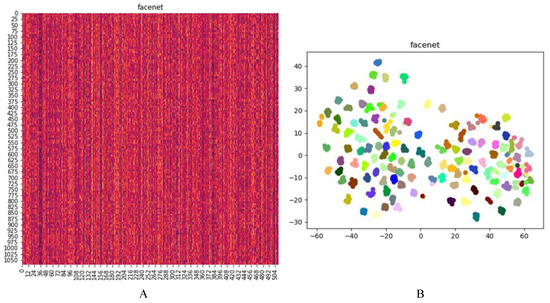
Figure 13.
(A) The heat map to represent training set in feature space, learned by Arcface. (B) The extracted vectors by FaceNet visualized in two dimensions space by t-SNE.
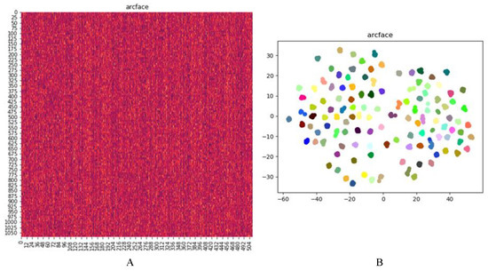
Figure 14.
(A) The heat map to represent training set in feature space, learned by Arcface. (B) The extracted vectors by Arcface visualized in two dimensions space by t-SNE.
Figure 15 shows smaller overlap area between inter-class (green) and intra-class (red) distance, the more discriminative power model has. With this overlap area, we can set a threshold to decide whether a feature of a test face belongs to a known-class or not. In our experiment, to minimize the false positive, we choose a threshold which return largest inter-class area and smallest intra-class area. We can clearly see that the overlap area of Arcface is much smaller compared to Facenet. With face description learned from Arcface, threshold around 1.07 can capture 98% face in a same class in training data. On the other hand, Facenet only found the best rate of 65% if we set threshold of 0.35.
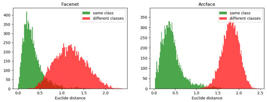
Figure 15.
Inter-class and intra-class distance of face representation computed by Facenet and Arcface.
We build four classifiers: SVM Linear Kernel (Linear SVM) [27], SVM RBF Kernel (RBF-SVM) [30], Gaussian Naive Bayes (NB) [27], and Weighted—KNN [31]. In this report, we only present the best results we obtained for each classifier. Table 1 shows the number of errors for each combination. In order to measure the performance of each method, we build a confusion matrix for each pair, denoted by . We then calculate the total error corresponding to each by the sum of all cells not belonging to the diagonal of the matrix, such that: .

Table 1.
The number of errors in the test set corresponds to the combination of the methods.
Through the numerical results obtained from Table 1, we can see the best results obtained from the combination of Feature extractor ArcFace and the classifier KNN. Table 1 shows the fusion matrix of the combination between different face embedding methods and classification methods.
We can see that when using Arcface as feature extraction, the result was excellent when combining some algorithms using similarity based on distance like KNN or Linear SVM. Because we do not have a definition of unknown class, so the predicted result P(y | x) is low. There are many samples in the scope of research but misclassified into the “unknown” class. These miss classifying is significantly improved when using the summarization process. Figure 16 illustrates the fusion matrix before executing summarization. Our setting archives an accuracy of 91.3% on the test dataset. The diagonal of the matrix has many zeros, which indicates that many students have been misidentified. The summarization algorithm has dramatically reduced the unwanted effects of the environment. The resulting output includes unqualified images obtained from the camera, which are synthesized and corrected by better quality images. In Figure 17, we show the confusion matrix of the system, and the accuracy is 92.7%. Although the efficiency only increases by 1.4%, the ratio of false positive decreased significantly to 1%. If we remove the unknown samples from our data, the accuracy can be up to 98.5%. The values of 0 on the diagonal line have replaced most. Our results almost reach the results of Arcface even we do not have standard conditions, and we get many difficulties as listed before in the school environment.
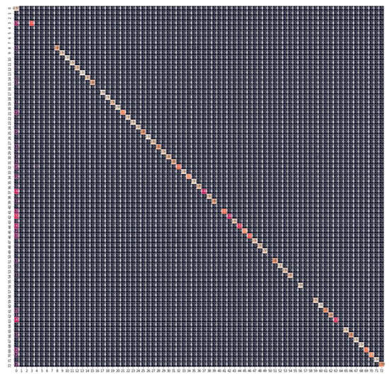
Figure 16.
Confusion matrix archived from the combination of Arcface (pre-trained model LResNet100E-IR, ArcFace@ms1m-refine-v2) and KNN (K = 5 and confident distance threshold = 1.07). The first column and row represent the label of “unknown,” other columns and rows show the result of corresponding class. Displayed data is normalized because of the large number of “unknown” samples.
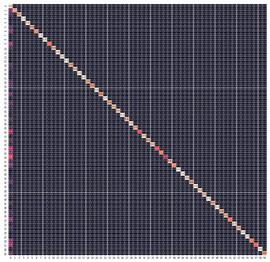
Figure 17.
The obtained confusion matrix after executing summarization process. The first column and row represent the label of “unknown,” other columns and rows show the result of corresponding class. Displayed data are normalized because of the large number of “unknown” samples.
3.3. System Processing Time
To enhance the computational power of the system, we used master-slaves architecture. Each instance of the above design implemented a separate process, so the job worker needs to be configured and assigned its address to perform hand-shaking with the job master. We set the data exchange method based on the Subscriber and Publisher pattern. This design allows us to make modifications to use different FR open-sources easily—the calculation speed is expected to increase linearly proportional to the number of job workers. The processing time of the system is not suitable for runtime responding. While detection and alignment are not too affected by the number of faces on the same frame, this dramatically affects the feature extractions (see Figure 18) and makes the performance decrease linearly. The predicted speeds of the classification models are breakneck, so are not presented in this section.

Figure 18.
(A) shows the processing time of the FR processing. (B) illustrate the processing time of face detection (including landmarks points) and face alignment. (C) visualizes the processing time of face description, corresponding to number of faces in the same.
Figure 19 shows the ability to utilize system resources to parallelly execut multiple jobs at the same time. As mentioned in Section 2.3.4, each attendance session lasts 25 min. We choose each job length to be 2 min. So if there are four cameras, it needs to be processed in ~802 s, so before check-out, students can receive attendance records at the time of their check-in. The system depends on the number of cameras connected. The computer configuration we used to measure the experiment was average. When using specialized workstations for deep learning, a CCTV system of hundred cameras with similar performance can be used. For a job worker, the system processes 12 videos in 1200 s, but when increasing the number of workers to 4, the processing time is reduced by only 1/3. The cause of this non-smooth is because the workers are running on the same PC, so they must share CPU and memory resources. This situation improves when using multiple PCs. Here we focus on proving flexibility to speed up the calculation.

Figure 19.
(A) total processing time on 12 videos using different number of workers. (B) CPU usage in percentage on 12 videos using different number of workers. (C) CPU usage in megabyte on 12 videos using different number of workers.
3.4. Application
As described above, the work of collecting data is difficult and essential in the construction of attendance systems. To accomplish this, we have built a mobile application that allows users to receive their faces. Figure 20 displays the screen captures of the data collector application. Students/academic staff use the mobile app to record the video containing the faces of a student. The video is then uploaded to the server for feature processing. Using the mobile application to collect face data dramatically reduces costs, and users can control their attendance information from the mobile app more efficiently than using a station. To modify the captured photos, the users need the license of the human resources department or training department. Attendees do not have the right to correct it themselves after they finish data collection for a duration.
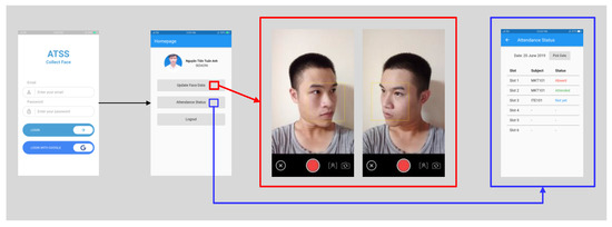
Figure 20.
Screen captures of mobile data collector application. Students/academic staff use mobile application to record the video-containing-faces of the student. Video then uploaded to server for feature processing.
We have received an assessment of the lecturers and quality assurance staff to monitor information about the entrance and exit time of the student during the session conveniently. The status of complaints about miss attendance decreased significantly compared to before the system put into use. Figure 21 shows the web page that an administrator can access to track attendance for a scheduled class. In the figure there are three students present with photos and time they appear in videos. In the picture, the “status” column shows the student’s current status, the “Images in video” column displays the student’s face image recorded in the video. The “Time Appeared in Video” column illustrates the time that the student identified in the video (this facility parameter allows the deduction of the student’s check-in time). Data from the system synchronized with the academic portal, so when there is a modification from the academic portal we will track through the “Actual Status” column, the default value is 0 (absent). During the test run, the system plays the role of support attendance taking system. The final decision made about whether or not a student is present in the class is still the faculty’s discretion. However, the reason for the differences is recorded.
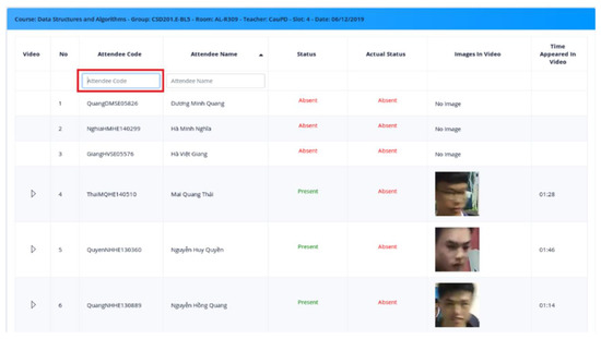
Figure 21.
A web page for tracking attendance based on the pre added schedule.
4. Conclusions
In this paper, we describe the architecture to build an automatic system for attendance taking using CCTV Camera. We illustrate the design by a case study at FPT Polytechnic. We showed the result of the real system and the feasibility of attendance taking support system in a university environment. In the experiment, the system worked with 120 students in five classes. We found out that it is impossible to achieve state-of-the-art accuracy of FR in the real environment. Still, we had improved efficiency using our algorithm using the movement of the face to remove some wrong results. It seemed promising and showed that we increase the effectiveness of our system. We propose a full system solution powered by state-of-the-art facial recognition model, from hardware to procedures for handling many streaming videos with unknown faces recorded by CCTV. By taking advantage of multi-process and job scheduling, we also leverage the hardware efficiency of face recognition to minimize system cost but still meet the required response time.
Although state-of-the-art shows the result of high accuracy with millions of objects, it is currently not possible to directly apply these techniques in the real world because of the difficulties of the real environment. When the number of attendees increased to thousands, this leads to a decrease in reliability and becomes the most significant risk of the attendance system. In our proposed method, the scheduling data plays the role of narrowing down the search scale when the system matches the student’s face with the face data. Therefore, when the number of users increases, it does not affect the performance of the FR module if the traffic moving through the CCTV does not change. The adaptation between the attendance system and existing information systems based on FR is vital.
Since attendance taking system required high precision, our policy is still struggling with low recall. It is a disadvantage if the test environments are not optimal. Concerning the results of our single classifiers, we can also expect to improve recall by not using a unique classifier technique. The combination of parametric (SVM, DNN) and non-parametric classifier (KNN) to better define “Unknown” class can increase the recall performance. Our system is also dependent on preprocessing. In the future, we can use some other models to improve our results. Currently, our system’s target can handle up to 500 students. However, because of some difficulty that we have mentioned above, we have evaluated our policy only on 120 students. Shortly, we will increase the size of the evaluation dataset to verify the comprehensiveness of our system.
In recent years, face recognition based on 3-dimensional data [32] has yielded incredible results compared to 2-dimensional image processing techniques. 3-dimensional spatial data brings more valuable information to describe the face [33]. However, to collect 3D data with existing devices is not an easy task. There are two ways to do this: (1) Use the RGB-D sensor—these sensors only need to be invested once. Still, currently, the 3D point-cloud data obtained from this type of sensor is dependent on the distance; it is greatly affected by sunlight conditions, not suitable for CCTV investment. (2) Using multiple 2D cameras [34], this method is not feasible because it requires a more significant investment, making it difficult to reuse the cameras invested for the original security purpose. In [35] Jiang, L. introduced a new approach to creating 3D data from a single 2D image. Although their results are promising, the method needs to be further studied with actual data. 3D based on FR is one of the directions our research would continue in the future, besides the performance improvement.
Author Contributions
N.T.S.: Conceptualization, Data curation, Formal analysis, Investigation, Methodology, Resources, Software; Visualization; Writing—original draft; Writing—review & editing; B.N.A.: Conceptualization, Data curation, Formal analysis, Investigation, Methodology, Resources, Software, Supervision; T.Q.B.: Data curation; Investigation; Methodology L.P.C.; Data curation; Investigation; Project administration; B.D.C.: Conceptualization; Funding acquisition; Methodology D.X.H.: Software, Visualization; L.V.T.: Software, Visualization; T.Q.H.: Software; L.D.D.: Software; M.H.R.K.: Formal analysis; Validation. All authors have read and agreed to the published version of the manuscript.
Funding
This research received no external funding.
Conflicts of Interest
The authors declare no conflict of interest.
References
- Minaee, S.; Abdolrashidi, A.; Su, H.; Bennamoun, M.; Zhang, D. Biometric recognition using deep learning: A survey. arXiv 2019, arXiv:1912.00271. [Google Scholar]
- Son, N.T.; Chi, L.P.; Lam, P.T.; Van Dinh, T. Combination of facial recognition and interaction with academic portal in automatic attendance system. In Proceedings of the 2019 8th International Conference on Software and Computer Applications (ICSCA ’19). ACM, New York, NY, USA, 19–21 February 2019; pp. 299–305. [Google Scholar] [CrossRef]
- Shoba, D.; Sumathi, C.P. A Survey on Various Approaches to Fingerprint Matching for Personal Verification and Identification. International Journal of Computer Science & Engineering Survey (IJCSES), 7 August 2016; Volume 7, No. 4. [Google Scholar] [CrossRef]
- Balaban, S. Deep learning and face recognition: The state of the art. arXiv 2015, arXiv:1902.03524. [Google Scholar]
- Yu, H.; Luo, Z.; Tang, Y. Transfer learning for face identification with deep face model. In Proceedings of the 2016 7th International Conference on Cloud Computing and Big Data (CCBD), Macau, China, 16–18 November 2016. [Google Scholar] [CrossRef]
- Wang, M.; Deng, W. Deep face recognition: A survey. arXiv 2019, arXiv:1804.06655v8. [Google Scholar]
- Deng, J.; Guo, J.; Zafeiriou, S. Arcface: Additive angular margin loss for deep face recognition. arXiv 2018, arXiv:1801.07698. [Google Scholar]
- Liu, W.; Wen, Y.; Yu, Z.; Li, M.; Raj, B.; Song, L. SphereFace: Deep hypersphere embedding for face recognition. In Proceedings of the 2017 IEEE Conference on Computer Vision and Pattern Recognition (CVPR), Honolulu, HI, USA, 21–26 July 2017. [Google Scholar] [CrossRef]
- Schrof, F.; Kalenichenko, D.; Philbin, J. FaceNet: A unified embedding for face recognition and clustering. arXiv 2015, arXiv:1503.03832V3. [Google Scholar]
- Wang, H.; Wang, Y.; Zhou, Z.; Ji, X.; Gong, D.; Zhou, J.; Liu, W. CosFace: Large margin cosine loss for deep face recognition. In Proceedings of the 2018 IEEE/CVF Conference on Computer Vision and Pattern Recognition, Long Beach, CA, USA, 16–20 June 2018. [Google Scholar] [CrossRef]
- Ranjan, R.; Sankaranarayanan, S.; Bansal, A.; Bodla, N.; Chen, J.C.; Patel, V.M.; Castillo, C.D.; Chellappa, R. Deep learning for understanding faces: Machines may be just as good, or better, than humans. IEEE Signal Process. Mag. 2018, 35, 66–83. [Google Scholar] [CrossRef]
- Zhang, K.; Zhang, Z.; Li, Z.; Qiao, Y. Joint face detection and alignment using multitask cascaded convolutional networks. IEEE Signal Process. Lett. 2016, 23, 1499–1503. [Google Scholar] [CrossRef]
- Wang, H.; Li, Z.; Ji, X.; Wang, Y. Face R-CNN. arXiv 2017, arXiv:1706.01061. [Google Scholar]
- Farfade, S.S.; Saberian, M.; Li, L.-J. Multi-view face detection using deep convolutional neural networks. arXiv 2015, arXiv:1502.02766. [Google Scholar]
- Feng, Z.-H.; Kittler, J.; Awais, M.; Huber, P.; Wu, X.-J. Face detection, bounding box aggregation and pose estimation for robust facial landmark localisation in the wild. In Proceedings of the 2017 IEEE Conference on Computer Vision and pattern Recognition Workshops, (CVPRW), Honolulu, HI, USA, 21–26 July 2017. [Google Scholar] [CrossRef]
- Sagonas, C.; Antonakos, E.; Tzimiropoulos, G.; Zafeiriou, S.; Pantic, M. 300 faces in-the-wild challenge: Database and results. Image Vis. Comput. 2016, 47, 3–18, Special Issue on Facial Landmark Localisation “In-The-Wild”. [Google Scholar] [CrossRef]
- Brinkmann, R. The Art and Science of Digital Compositing; Morgan Kaufmann: Burlington, MA, USA, 1999; p. 184. ISBN 978-0-12-133960-9. [Google Scholar]
- Han, J.; Kamber, M.; Pei, J. Data Mining: Concepts and Techniques, 3rd ed.; Morgan Kaufmann Publishers Inc.: San Francisco, CA, USA, 2011. [Google Scholar]
- Course Syllabus EBIO 6300: Phylogenetic Comparative Methods-Fall 2013. Available online: https://www.colorado.edu/smithlab/sites/default/files/attached-files/EBIO6300_PCMsSyllabus.pdf (accessed on 1 June 2019).
- Space and Naval Warfare Systems Center Atlantic. CCTV Technology Handbook; System Assessment and Validation for Emergency Responders (SAVER), 2013.
- Zhou, Y.; Liu, D.; Huang, T. Survey of face detection on low-quality images. In Proceedings of the 2018 13th IEEE International Conference on Automatic Face & Gesture Recognition (FG 2018), Xi’an, China, 15–19 May 2018. [Google Scholar] [CrossRef]
- Masi, I.; Wu, Y.; Hassner, T.; Natarajan, P. Deep face recognition: A survey. In Proceedings of the 2018 31st SIBGRAPI Conference on Graphics, Patterns and Images (SIBGRAPI), Foz do Iguaçu, Brazil, 29 October–1 November 2018. [Google Scholar] [CrossRef]
- Ngoc Anh, B.; Tung Son, N.; Truong Lam, P.; Phuong Chi, L.; Huu Tuan, N.; Cong Dat, N.; Huu Trung, N.; Umar Aftab, M.; Van Dinh, T. A computer-vision based application for student behavior monitoring in classroom. Appl. Sci. 2019, 9, 4729. [Google Scholar] [CrossRef]
- Li, J.; Zhang, D.; Zhang, S. The application and research on master-slave station distributed integration business architecture. In Proceedings of the 2016 IEEE Advanced Information Management, Communicates, Electronic and Automation Control Conference (IMCEC), Xi’an, China, 3–5 October 2016. [Google Scholar] [CrossRef]
- Wang, X.; Wang, K.; Lian, S. A survey on face data augmentation. arXiv 2019, arXiv:1904.11685. [Google Scholar]
- Ruiz, N.; Chong, E.; Rehg, J.M. Fine-grained head pose estimation without keypoints. In Proceedings of the IEEE Conference on Computer Vision and Pattern Recognition (CVPR) Workshops, Salt Lake City, UT, USA, 18–22 June 2018; pp. 2074–2083. [Google Scholar]
- Murphy, K.P. Machine Learning: A Probabilistic Perspective, 1st ed.; Adaptive Computation and Machine Learning series; MIT Press: Cambridge, MA, USA, 2012. [Google Scholar]
- Yilmaz, A.; Javed, O.; Shah, M. Object tracking: A survey. ACM Comput. Surv. 2006, 38. [Google Scholar] [CrossRef]
- Van der Maaten, L.; Geoffrey, H. Visualizing data using t-SNE. J. Mach. Learn. Res. 2008, 9, 2579–2605. [Google Scholar]
- Wang, J.; Chen, Q.; Chen, Y. RBF kernel based support vector machine with universal approximation and its application. In Advances in Neural Networks—ISNN 2004; Yin, F.L., Wang, J., Guo, C., Eds.; Lecture Notes in Computer Science; Springer: Berlin/Heidelberg, Germany, 2004; Volume 3173, ISNN 2004. [Google Scholar]
- Hechenbichler, K.; Schliep, K. Weighted K-Nearest-Neighbor Techniques and Ordinal Classification; Discussion paper 399; SFB 386; Ludwig-Maximilians University: Munich, Germany, 2004; Available online: http://www.stat.uni-muenchen.de/sfb386/papers/dsp/paper399.ps (accessed on 25 June 2019).
- Zhou, S.; Xiao, S. 3D face recognition: A survey. Hum. Cent. Comput. Inf. Sci. 2018, 8, 35. [Google Scholar] [CrossRef]
- Marcolin, F.; Violante, M.G.; Sandro, M.O.O.S.; Vezzetti, E.; Tornincasa, S.; Dagnes, N.; Speranza, D. Three-dimensional face analysis via new geometrical descriptors. In Lecture Notes in Mechanical Engineering; Springer: Cham, Switzerland, 2017; pp. 747–756. [Google Scholar] [CrossRef]
- Widanagamaachchi, W.N.; Dharmaratne, A.T. 3D Face Reconstruction from 2D Images. In Proceedings of the 2008 Digital Image Computing: Techniques and Applications, Canberra, ACT, Australia, 1–3 December 2008; pp. 365–371. [Google Scholar] [CrossRef]
- Jiang, L.; Zhang, J.; Deng, B.; Li, H.; Liu, L. 3D face reconstruction with geometry details from a single image. IEEE Trans. Image Process. 2018, 27, 4756–4770. [Google Scholar] [CrossRef] [PubMed]
© 2020 by the authors. Licensee MDPI, Basel, Switzerland. This article is an open access article distributed under the terms and conditions of the Creative Commons Attribution (CC BY) license (http://creativecommons.org/licenses/by/4.0/).