An Improved Network Traffic Classification Model Based on a Support Vector Machine

Abstract

Network traffic classification based on machine learning is an important branch of pattern recognition in computer science. It is a key technology for dynamic intelligent network management and enhanced network controllability. However, the traffic classification methods still facing severe challenges: The optimal set of features is difficult to determine. The classification method is highly dependent on the effective characteristic combination. Meanwhile, it is also important to balance the experience risk and generalization ability of the classifier. In this paper, an improved network traffic classification model based on a support vector machine is proposed. First, a filter-wrapper hybrid feature selection method is proposed to solve the false deletion of combined features caused by a traditional feature selection method. Second, to balance the empirical risk and generalization ability of support vector machine (SVM) traffic classification model, an improved parameter optimization algorithm is proposed. The algorithm can dynamically adjust the quadratic search area, reduce the density of quadratic mesh generation, improve the search efficiency of the algorithm, and prevent the over-fitting while optimizing the parameters. The experiments show that the improved traffic classification model achieves higher classification accuracy, lower dimension and shorter elapsed time and performs significantly better than traditional SVM and the other three typical supervised ML algorithms.

1. Introduction

With the dramatic growth in network applications, the current network has become a large, dynamic and complex system. Large-scale network applications have brought serious challenges to management. Therefore, network management based on traffic analysis intelligently is an urgent task. The network traffic classification is the foundation of network management, which can manage the corresponding network traffic differently, provide the basis for the subsequent network protocol design, provide the methods for network attack detection and flow cleaning in network security [1].

There are four main methods of traffic classification research at present [2,3,4]: port numbers-based method, deep packet inspection (DPI) method [5,6], protocol analysis method and machine learning techniques. Since 2001, the number of research papers in the field of network traffic classification has increased year over year. With the increase of network traffic and the backbone network optimization, the current network traffic classification method can’t completely solve all kinds of problems caused by the constant change of traffic characteristics. For the machine learning techniques are intelligent and flexible, more and more researches on network traffic classification are focused on this field in recent years. At the same time, the traffic classification method based on machine learning also faces some challenges: (1) The optimal feature subset is difficult to obtain. The classification method needs an effective feature combination to form the optimal feature subset so that the classification algorithm can get the maximum classification accuracy. Meanwhile, it is expected that the feature set contains the least number of features, and effectively removes redundant and irrelevant features. (2) The high dimensional feature results in high computational complexity and long convergence time of the machine learning classification algorithm. If traffic features are extracted from the traffic packet header, when the number of packets extracted from each traffic feature is equal to ($n$), the cost of collecting and calculating each feature is close to $O$($n{\log }_2^n$). (3) The traffic classification accuracy is highly correlated with the prior probability of training samples. While the training and test samples in the classification model may be biased to partial flow. (4) Some classification models, such as C4.5 decision tree, or K-Nearest Neighbor (K-NN) is easy to fall into local optimum.

In summary, it is a challenge to realize network traffic classification by machine learning. No doubt that there are great theoretical significance and application value to apply it to network traffic classification. In this paper, we focus on reducing the dimension of the flow features and deriving the optimal working parameters based on the machine learning model. The major contributions of this work are summarized as follows:

(1)

In the process of feature reduction, in order to select the optimal feature subset which can represent the distribution of original traffic data, a Filter-Wrapper hybrid feature selection model is proposed.

(2)

In order to balance the empirical risk and generalization ability of support vector machine (SVM) traffic classification model, improve its classification and generalization ability, and improved the grid search parameter optimization algorithm is proposed. The algorithm can dynamically adjust the second search area, reduce the density of grid generation, improve the search efficiency of the algorithm, and prevent the over-fitting while optimizing the parameters.

(3)

We compare the proposed model with the traditional SVM, and the representative supervised machine learning algorithm. It shows that traffic classification performance can be significantly improved by the proposed model by using very few training samples.

The rest of the paper is organized as follows: Section 2 reviews the related work of traffic classification. Section 3 describes the proposed methods and framework. Section 4 proposes an experimental framework and a detailed performance evaluation of the proposed model. Section 5 draws a conclusion.

2. Related Works

2.1. Method Based on Port Numbers

Port-based traffic classification is mainly used in early typical applications. The Internet Assigned Numbers Authority (IANA) plans corresponding TCP/UDP service ports for each application in the network. The main limitations are as follows: (1) Some open ports are applied to different networks. (2) In order to pass through firewalls and avoid sniffing, some applications use port confusion technology to fake the default ports of other applications [7].

2.2. Method Based on Deep Packet Inspection

Traffic classification based on deep packet inspection (DPI) is a method with high classification accuracy [8]. DPI traffic classification not only detects IP and TCP/IP header but also detects part or all the payload of the data packet, which is called depth packet inspection. Although the accuracy of traffic classification based on DPI is high, this method still has some defects: (1) As the number of non-standard applications and private protocols increases more and more, these applications and protocols lack applicable and open standards, which makes feature strings changeful and difficult to inspect [9]. (2) The random encrypted stream in some network traffic associates several characteristic strings, which makes the false-positive increase.

2.3. Method Based on Protocol Analysis

Based on open protocol regulations, protocol analysis methods analyze the protocols by establishing protocol state machines for traffic classification. Iliofotou et al. [10] classify traffic by analyzing the behavior characteristics of network applications and provides the concept of traffic dispersion graphs (TDGs). The TDG inspection method can be used to analyze and visualize network traffic. In addition, the features of Skype client are analyzed by using private communication and encrypted data traffic, Bonfiglio et al. [11] proposed to identify the traffic of the Skype client through some features of the client. Although the efficiency of traffic classification based on protocol analysis is better than those based on DPI, it still faces some challenges: (1) It is difficult to analyze the effective features of the non-standard application and encryption protocol traffic. (2) The analysis of the protocol is based on the current version of the protocol. Once the version of the protocol is revised, the features of the protocol will change, so it is necessary to analyze the protocol again.

2.4. Method Based on Machine Learning Techniques

The machine learning methods capture and identify the traffic data packets based on calculating the statistical information of the specific application traffic. Machine learning methods mainly include supervised learning and unsupervised learning. Classifier builds unsupervised learning based on clustering samples according to their similarity rather than labeling the training set in advance. There are many representative clustering algorithms, such as K-means [12,13] clustering (K-means), expectation-maximization (EM) [14], etc. The supervised learning is more favorable to the construction of an application-oriented network traffic classification model because it knows the actual traffic categories. Supervised learning refers to the design of classification models and parameters based on prior knowledge. In supervised learning algorithms, classifiers or classification models are based on certain pattern recognition techniques, such as Bayesian, C4.5 decision tree, and K-NN, which are easy to fall into local optimization. In addition, Ensemble learning is a method of using several basic classifiers to execute decisions together [15]. The basic classifiers include such as decision tree, random forest, Bayesian, etc. [16]. However, the dependencies between the basic classifiers and the number of basic classifiers need to be determined, the generalization ability and classification performance of ensemble learning algorithms will be greatly affected. Deep learning is a characterization learning method based on the data in machine learning [17]. Though the training of deep learning depends on the huge amount of training data heavily, and the hyper-parameters optimization of deep neural networks is difficult [18]. In the above methods, the support vector machine (SVM) algorithm is a kind of supervised learning algorithm based on statistical theory [19]. And based on the kernel function transformation and structural risk minimization (SRM) principle, the traffic classification is transformed into a quadratic optimization problem, which has good classification accuracy and stability. Moreover, it is more capable to solve high dimensional nonlinear problems [20]. In recent years, the research of network traffic classification based on SVM is the focus of supervised learning with theoretical significance and practical application value. In reference [21], a maximum margin SVM is proposed to avoid local optimization, and a discriminatory selection algorithm is proposed. In [22], a method of extracting and determining traffic parameters from the packet header was proposed based on SVM. Bulk, interactive, WWW, service, P2P, and other application traffic were classified. For biased samples, the overall average classification accuracy is 99.41%. And for unbiased samples, the overall average classification accuracy is 92.81%. To sum up, the supervised classification method based on SVM has been widely used in feature selection, classification of network traffic and other research fields. With the development of SVM theory, it is more and more urgent to apply it to do network traffic feature selection and traffic classification. Therefore, the main research content of this paper is to study the characteristics and application scope of the SVM training model, then propose reasonable feature selection, traffic classification methods and corresponding solutions.

3. Materials and Methods

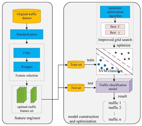
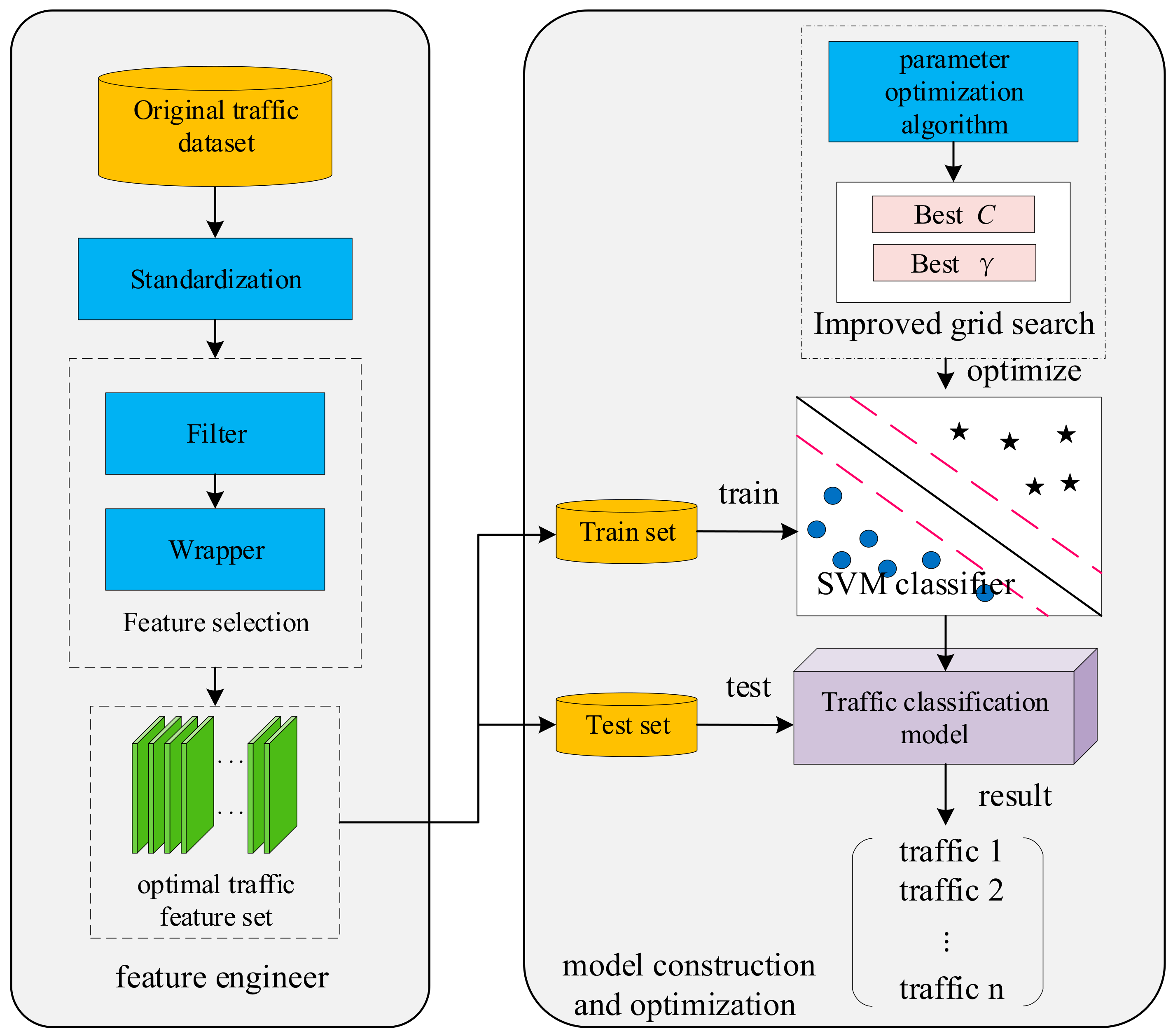
3.1. Model Framework

We proposed an improved network classification model based on SVM, this model improves the accuracy of traffic classification. The model contains two modules, they are feature engineer and classifier building. First, we proposed a filter-wrapper mixed feature selection algorithm, obtain the optimal feature set to represent the original feature set. And then we proposed an improved grid search algorithm, the algorithm gets the best combination of the key parameter of SVM classifier to improve the classification accuracy and prevent overfitting. The model framework is shown in Figure 1.

Figure 1. The improved network traffic classification based on SVM.

3.2. The Filter-Wrapper Feature Selection Algorithm

Although filter feature selection is independent of the machine learning algorithm, it has low computational complexity and fast feature selection speed. But it also has some limitations: (1) Redundant features can’t be completely removed. When a redundant feature is highly correlated with the target class, the feature will not be removed completely. (2) The ability of combination feature selection is poor. When some feature combinations appear, they will have a strong ability to distinguish, and there is a certain correlation between these features. The filter feature selection often only selects one or several of them. The other combined features with strong distinguishing ability are filtered out as redundancy. (3) As selecting the optimal feature subset is based on the information and statistical features of the data, and independent from the learning algorithm, the classification effect is often not very ideal.

Wrapper feature selection depends on the learning algorithm. The classification accuracy will reach a higher level. But it also has some limitations: (1) The computational complexity is high relatively. When there are n dimension features and the number n is large, an exhaustive subset of 2ⁿ features will cause the NP problem [23]. In addition, when the k-fold crossover is used to verify the classification accuracy of the feature subset, the computational complexity is huge. (2) It is often necessary to combine the optimal search strategy to obtain the approximate optimal feature subset.

3.2.1. Filter-Wrapper Feature Selection Model Framework

In order to overcome the limitations of the traditional feature selection, we propose a filter-wrapper hybrid feature selection model. The model framework is shown in Figure 2. The process of feature selection in this model is as follows: (1) The pre-processed data set $S_0$ is first selected by the filter. The information gain (IG) algorithm is used to evaluate the information gain of each feature that contributes to the classification, and a heuristic optimal feature selection search strategy is used to sort the IG value of the feature attribute. Finally, a new candidate feature subset $F_1$ is obtained by removing the feature whose weight is less than the set threshold $\delta$ from the original dataset. (2) Wrapper second feature selection is performed on the candidate feature subset $F_1$ and data set $S_1$. Based on the SVM learning algorithm and heuristic sequence forward search strategy, an optimal feature subset $F_2$ with high classification accuracy is selected. (3) The data set $S_2$ which is composed of the optimal feature subset $F_2$ selected by the Filter-Wrapper model is divided into a training set and test set. Then based on the training of the SVM classifier, the network traffic classification results are obtained on the test set.

Figure 2. Filter-wrapper hybrid feature selection model based on SVM.

This filter-wrapper hybrid feature selection model reduces the feature dimension of traffic sample space, shortens the training time and improves the classification performance of SVM. Because the second wrapper feature selection is based on the filter feature selection, the model overcomes the problem of not considering the combination feature ability and the poor classification effect caused by using the filter feature selection model only. At the same time, due to the filter feature subset selection, the computational complexity of the wrapper second feature selection is greatly reduced and the classification effect is ideal.

3.2.2. Filter-Wrapper Feature Selection Algorithm Framework

The filter-wrapper hybrid feature selection algorithm framework is shown in Figure 3. The hybrid feature selection model can select the input feature set, reduce the dimension and improve the classification performance. $F_0\left(f_1,f_2,\dots ,f_i,\dots ,f_n\right)$ represents the scaling original feature set, $S_{filter}\leftarrow search\left(F_0\right)$ represents the Filter feature selection stage. Heuristic optimal feature combination search strategy is used to search candidate feature subsets $F_1$ in feature space $F_0$. And $E_{IG}\leftarrow evaluate\left(S_{filter},F_0\right)$, means to evaluate candidate feature subsets $F_1$ by information gain evaluation strategy.$E_{IG\_best}$ is the best evaluation value for $E_{IG}$. If $E_{IG}<E_{IG\_best}$ updates the evaluation value $E_{IG}$ and the candidate feature subset $F_1$ of the Filter selection, otherwise it is not updated. Loop the process until the threshold ${\delta }_{filter}$ termination conditions ${\delta }_{stop\_filter}$ are satisfied (${\delta }_{filter}={\delta }_{stop\_filter}$), finish the Filter feature selection process, and output the target feature subset $F_1\left(f_1,f_2,\dots ,f_i,\dots ,f_{n*}\right)$, $n*<n$ of the feature selection in this stage. $S_{wrapper}\leftarrow search\left(F_1\right)$ indicates that in the wrapper feature selection. A heuristic sequence forward search strategy is used to search candidate feature subsets $F_2$ in the feature space $F_1$.$E_{svm\_test}\leftarrow evaluate\left(S_{wrapper},F_1\right)$, means that after the training model is established by the SVM classification algorithm, the candidate feature subset $F_2$ is tested. On the test set, if the accuracy $Tes{t}_{accuracy}$ is higher than the previous best accuracy $Tes{t}_{best}$($Tes{t}_{accuracy}>Tes{t}_{best}$), the evaluation value $E_{svm\_test}$ and the wrapper candidate feature subset $F_2$ are updated by the best SVM evaluation value $E_{svm\_test\_best}$ and the best feature subset $F_{best}$. Otherwise, no updates are made. The process is circularized until the threshold is satisfied and the wrapper feature selection is completed. Then the target feature subset $F_2\left(f_1,f_2,\dots ,f_i,\dots ,f_m\right)$ of the feature selection is outputted and the feature dimension is $m$.

Figure 3. Filter (IG) feature selection process.

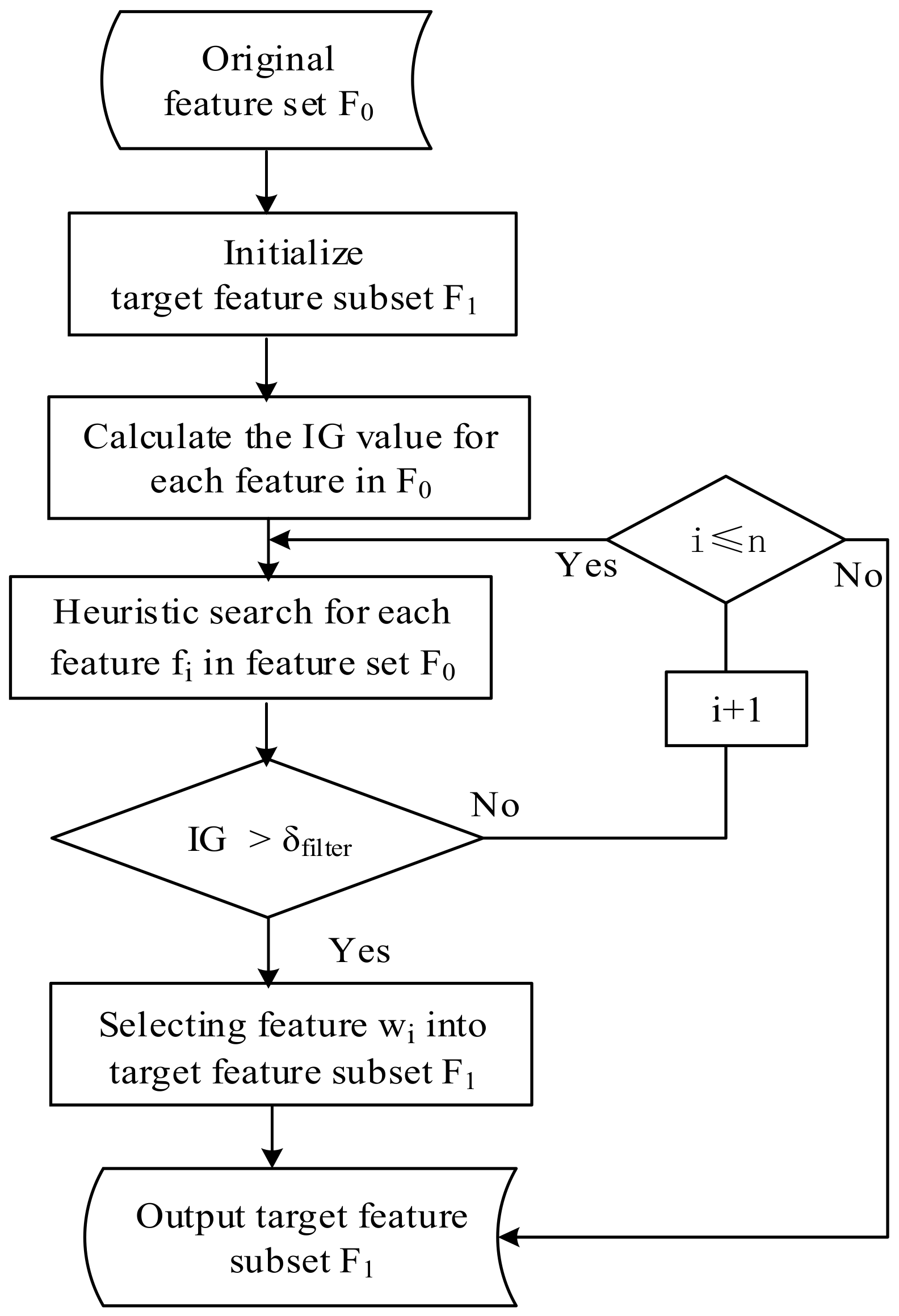
3.2.3. Filter Feature Selection Algorithm Evaluation Strategy

In the hybrid feature selection algorithm, the wrapper second feature selection directly uses the SVM classifier as the evaluation strategy, which means the feature subset is evaluated based on the classification performance of SVM. In the filter feature selection stage, the information gain (IG) algorithm is used as the evaluation strategy which is independent of the learning algorithm. IG is an entropy evaluation method, which evaluates the information gain of each feature that contributes to the classification. The more information a variable has, the greater the entropy. If the corresponding probability of the class feature variable $S\left(S_1,S_2,\dots S_n\right)$ is $P\left(P_1,P_2,\dots P_n\right)$, then the entropy $S$ is shown on Equation (1). The IG of attribute feature $F\left(f_1,f_2,\dots f_n\right)$ is the difference of information quantity with and without $F$. The IG is shown on the Equation (2). $P\left(S_i\right)$ is the probability of the appearance of class $S$. $P\left(S_i|f_i\right)$ is the conditional probability that attributes feature $f_i$ belongs to category $S_i$. $P_i\left(S_i|\overline{f_i}\right)$ is the conditional probability of not having attribute feature $f_i$ and belonging to a class $S_i$. The larger value of $IG\left(F\right)$, the greater contribution of $F\left(f_1,f_2,\dots f_n\right)$ to classification. The information gain related to the class is sorted by the feature attribute. The higher the IG value of attribute feature, the greater its contribution to the classification:

$$H(S)=-{\displaystyle \sum _{i=1}^n{P}_i{\log }_2{P}_i}$$

(1)

$$\begin{array}{ll}IG\left(F\right)& =H\left(S\right)-H\left(S|F\right)\\ & =-{\displaystyle \sum _{i=1}^{n}P\left(S_i\right){\log }_{2}P\left(S_i\right)+P\left(f_i\right){\displaystyle \sum _{i=1}^{n}P}\left(S_i|f_i\right){\log }_2}P\left(S_i|f_i\right)\\ & +\mathrm{P}\left(\overline{f_i}\right){\displaystyle \sum _{i=1}^{n}P}\left(S_i|\overline{f_i}\right){\log }_{2}P\left(S_i|\overline{f_i}\right)\end{array}$$

(2)

According to the IG value of each traffic feature in the Equation (2), combining the heuristic optimal feature selection search strategy, the feature IG value is sorted, and the feature which threshold ${\delta }_{filter}=0$ is filtered out to form a new candidate feature subset $F_1$. The feature selection process is shown in Figure 4.

Figure 4. Filter (IG) feature selection process.

The input is the original feature set $F_0$. The target feature subset $F_1$ is initialized. The IG value of each feature $f_i$ is calculated according to Equation (2). Each feature $f_i$ is searched in the feature set $F_0$ and sorted according to the IG value of the feature. When the IG value is less than or equal to the threshold ${\delta }_{stop\_filter}\left({\delta }_{stop\_filter}=0\right)$, the feature $f_i$ is deleted and the next feature is searched. When the IG value is greater than the set threshold ${\delta }_{stop\_filter}$, the searched feature $f_i$ is selected into the target feature subset $F_1$. The loop search processes until the last feature $f_n$ in the feature set $F_0$ are searched, then the search process is completed, and the final target feature subset $F_1$ is output.

3.2.4. Wrapper Feature Selection Algorithm Search Strategy

The filter feature selection process adopts a heuristic single optimal feature combination search strategy. The IG values of a single feature in the feature set are sorted and selected according to the set threshold. The k best features are combined to form a candidate feature subset. Although the single optimal feature combination strategy does not consider the interdependence between features, its efficiency is high, which is very suitable for the initial feature selection of the filter-wrapper hybrid feature selection algorithm. The computational complexity of the later wrapper feature selection stage is greatly reduced. The combination feature ability and the classification effect can be realized in the wrapper second feature selection stage.

In the wrapper second feature selection stage, the heuristic sequence forward selection search strategy is used to obtain the approximate optimal feature subset. The main idea of this strategy is: starting from the empty set, one or more features that can make the classifier of candidate subset with the highest accuracy, are added to the current feature candidate subset until the number of features exceeds the total number of features (threshold). That is, starting from the initial feature space (empty set), each time we select m features from the feature space of filter feature selection, add them into $F_1$ to generate a new candidate feature subset F₂ until the constraint conditions are satisfied. The heuristic search adopts the depth-first strategy. When the maximum diameter of the search is N, the computational complexity is O(N), which reduces the computational cost of the search.

Search strategy description: select an empty set as the initial feature subset $F_1$. From the traffic feature space $F\left(f_1,f_2,\dots ,f_i,\dots ,f_{n*}\right)$ of Filter feature selection, the selected $k$ features are added to the initial feature set $F_1$. The classification accuracy $A_0$ of $S_1$ in $F_1$ was calculated after filter feature selection, and the candidate feature subset $F_2$ was generated by $F_1$. The sequence forward selection was used. The loop selects $m$ features from the remaining features and adds them to $F_1$. Finally, a new candidate feature $F_2$ is generated. The classification accuracy $A_1$ on $F_2$ is calculated and compared with $A_0$. If $A_1>A_0$, then the feature subset $F_1$ is updated. So that $F_1=F_2$. Otherwise, $F_1$ will not be updated. When the feature number $i$ cannot satisfy the threshold condition, that is, $i$ exceeds the maximum number of features, then all the features are cyclically searched, and the algorithm ends. The specific algorithm framework is shown in Algorithm 1.

Algorithm 1: Heuristic Sequence Forward Search Strategy

Input: initial feature set $F_1$

Output: target feature set $F_2$

1. $F_1\leftarrow \varnothing$;

2. Select $k$ features to add into the initial feature set $F_1$;

3. For $i\le {\delta }_{wrapper}$ do

4.   The classification accuracy $A_0$ of computing data set $S_1$ on $F_1$;

5.   Select $m$ features from the remaining features and add them into $F_1$ to generate a new feature subset $F_2$;

6.   The classification accuracy $A_1$ of computing data set $S_1$ on $F_2$;

7.    if$A_1>A_0$, then$F_1=F_2$;

8.    else, $F_1$ no change;

9.    End if

10. End For

3.3. Parameters Optimization Based on Improved Grid Search Algorithm

3.3.1. Basic Principle of Traditional Grid Search Algorithm

The grid search algorithm (GS) [24] is one of the commonly used methods to optimize SVM parameters. The main principle is as follows: If it contains n parameters, (1) For grid division in the n-dimensional parameter space, each candidate parameter combination is represented by a grid node. (2) Set the value range of each parameter $y_i$ and sample according to the specified step size. Generate a set $U\left(y_i\right)=\left\{U\right.\left(y_i\right)\times U\left(y_2\right)\times \dots \times \left.U\left(y_n\right)\right\}$ of parameter samples, that is, generating grids according to the different directions of the parameter $y_i$. (3) For each parameter sample $y_i$ (grid node), the corresponding evaluation method is used until all the parameter samples are evaluated. Output optimal parameter combination.

The grid search algorithm is simple in principle, which has no correlation between grid nodes and has strong generality. In theory, when the search space is large enough and the search step is small enough, the global optimal solution can be found. In practical application, grid search is still a commonly used parameter optimization method [25,26]. However, as the parameters increase, the search space expands and the search step decreases, the grid becomes very dense and the computational overhead of the algorithm increases, especially when dealing with the large-scale data of network traffic. In this section, an improved Grid algorithm for optimizing SVM parameters is proposed. The algorithm can determine the global approximate optimal solution by finite search, reduce the computation cost, and improve the classification performance and generalization ability of SVM.

3.3.2. Improved Grid Search Algorithm Framework

SVM is to maximize the classification interval to achieve the best generalization ability. When the optimal classification plane can’t separate completely the two kinds of points, SVM allows the existence of error samples by introducing a relaxation factor $x_i$, which can balance the empirical risk and generalization ability of SVM. In this case, the classification plane satisfies: $y_i\left(w^T\varphi \left(x_i\right)+b\right)\ge 1-{\xi }_i$, when $0<{\xi }_i<1$, sample point $x_i$ is correctly classified, and when ${\xi }_i\ge 1$, sample point $x_i$ is misclassified. Therefore, the penalty term $C{\displaystyle \sum _{i=1}^l{\xi }_i}$ is added, the minimization objective function is the Equation (3), and $C$ is the penalty factor. The function of the penalty parameter $C$ is to adjust the tolerance of SVM to error samples when constructing the optimal classification plane. The appropriate $C$ value can balance the empirical risk and generalization ability of SVM:

$$\underset{w,b,\xi }{\min }\frac{1}{2}{w}^{T}w+c{\displaystyle \sum _{i=1}^l{\xi }_i}$$

(3)

At the same time, the parameter $\gamma =\frac{1}{\sigma }$ of the RBF kernel function affects the radial action range of the kernel function. When the scale parameter $\sigma$ is small, then $\sigma$ is smaller than the interval of actual training sample points, and the RBF kernel function $\exp {(-\gamma ‖x_i-x_j‖)}^2$ value is smaller so that the kernel function can only affect the samples in the small scale range where the sample interval is the same as $\sigma$. Therefore, setting the appropriate scale parameter $\sigma$, that is, determining the appropriate parameter $\gamma$ of the RBF kernel function, will have a great influence on the classification and generalization ability of the SVM. In this section, the Improved Grid Search algorithm (IGS) is used to optimize the SVM penalty parameters $C$ and the RBF kernel function parameters $\gamma$. The framework of the algorithm is shown in Algorithm 2. The details are as follows.

Algorithm 2: Improved Grid Optimization Parameter Algorithm (IGS)

Input:$\alpha$, $\beta$, $l_{cstep}$, $l_{\gamma step}$, $\delta$, $K$;

Output:$C_{best}$, ${\gamma }_{best}$, $C{V}_{best}$;

1. $\left[C_{\min },C_{max}\right]\leftarrow \left[2^{-\alpha },2^{\alpha }\right]$, $\left[{\gamma }_{\min },{\gamma }_{max}\right]\leftarrow \left[2^{-\beta },2^{\beta }\right]$;

2. $l_{cstep},l_{\gamma step}\leftarrow \lambda ·l\left(\lambda \ge 1\right)$;

3. The initial optimization result $C_{i1}$, ${\gamma }_{i1}$, $C{V}_{i1}$ is obtained by searching in the initial parameter space;

4. $l_{cstep}$, $l_{\gamma step}\leftarrow \frac{l}{2}$;

5. If $C_{i1}<\delta$, then

6.   Second-search of optimal contour region based on $C{V}_{i1}$ evaluation results;

7.   The second optimization results $C_{i2}$, ${\gamma }_{i2}$, $C{V}_{i2}$ are calculated and obtained;

8.   While $C_{i1}\ge \delta$ do

9.      For, $i=1\mathrm{to}2\alpha$, $j=1\mathrm{to}2\beta$ do

10.     $\left[C_{\min },C_{max}\right]\leftarrow \left[2^{-\alpha +i},2^{\alpha -j}\right]$, $j=1\mathrm{to}2\beta$;

11.     Calculate and update the second-optimization results $C_{i2}$, ${\gamma }_{i2}$, $C{V}_{i2}$;

12.     if $C_{i2}<\delta$, break

13.     $i+1$, $j+1$;

14.      End For

15.   End While

16. End if

17. $C_{best}\leftarrow C_{i2}$, ${\gamma }_{best}\leftarrow {\gamma }_{i2}$, $C{V}_{best}\leftarrow C{V}_{i2}$;

(1) In the initial parameter space $\left(C_i,{\gamma }_i\right)$, the IGS algorithm will increase the initial step size to $\lambda$ times of the default step $l$, that is, $\lambda ·l\left(\lambda \ge 1\right)$, and perform the initial traversal search until all the parameter samples are evaluated according to the evaluation method. The optimal parameter combination $\left(C_{i1},{\gamma }_{i1}\right)$ of SVM and the corresponding contour map of the evaluation result is outputted. Here the initial step size is increased to $\lambda ·l$, which can reduce the initial Grid search time and the density of the initial Grid generation.

(2) When the initial penalty parameter C is judged, if it does not exceed the critical value $\delta$, then reduce the search area according to the range of contour line with the highest evaluation value. And when the reduction step size is half of the default step $l$, the second search is carried out. If $C$ exceeds the critical value $\delta$ of over-fitting, then the boundary of the contour with the highest evaluation result can be searched twice in the opposite direction to the lower value of the evaluation result, until $C$ is within the limit of the critical value. After all the parameter samples are evaluated according to the evaluation method, the optimal parameter combination $\left(C_{i2},{\gamma }_{i2}\right)$ of SVM and the corresponding evaluation results are finally outputted. Here, the step size is reduced to increase the density of grid generation and to perform fine searches. When $C$ exceeds the critical value $\delta$, the algorithm searches for the lower value of the evaluation result in the opposite direction, in order to optimize the parameters, avoid over-fitting and improve the generalization ability of SVM.

3.3.3. IGS Evaluation Strategy

Based on statistical theory, the cross-validation (CV) method is used to evaluate samples. This method can effectively evaluate the performance of a classifier. The typical model is $k$-fold cross-validation ($k$-CV). The basic idea of k-fold cross-validation ($k$-CV) is to divide the training set into k subsets, and select each subset as the test set in turn, and the remaining k-1 subsets as training sets. The classification model trained by k-1 training sets is used to predict the corresponding test sets. After k times of training iteratively, the sum of the k-times prediction results are divided by the total number of samples to evaluate the generalization ability of the classification model. In k-fold cross-validation (k-CV), each sample is used as a test sample once and k-1 as training sample, which makes the evaluation results more reliable. At present, in the field of parameter optimization, although k-CV evaluation method is time-consuming, its principle is simple and reliable, which is still applied by many researchers in practice [27,28].

In (k-CV), the k value determines the generalization ability of the model. When the value k is small, the model with better prediction ability can’t be obtained. When the value k is larger, the calculation load of the model will increase sharply. Therefore, in the paper, we discuss the k value and determine a reasonable k value, so as to obtain a more effective and reliable evaluation method for predicting the ability of the SVM classification model.

4. Experimental Performance Evaluation

4.1. Datasets

In order to test and analyze the performance of feature selection model, the common real data sets are used to test, and the experimental results are compared and analyzed. The data set is Andrew Moore [29] data set, which is a collection of traffic collected by Moore et al. It contains 10 (24 h) data subsets of 1Gbps full-duplex network traffic. The collection time of each data subset is the 1680S (28 min), which contains 355,241 pieces of data and 248 attributes. Each line of each subset file represents network traffic, and each network traffic consists of packets with the same attributes.

The original data set is an unbalanced data set. The data amount of WWW and mail traffic flows reaches tens of thousands or even hundreds of thousands, but the games and interactive traffic flow data is only 118. In order to avoid the imbalance of data, two kinds of samples, games and interactive, are deleted. The original data set is sampled. On 10 classes of traffic data, equal proportions of random data are sampled for each subset with a sample number of less than 3000. Then, the sample data of 10 subsets are merged to form the experimental data set of 24897 samples, as shown in Table 1.

Table 1. Datasets.

Traffic Class	Representative Application	Sample of Flows	Traffic Class	Representative Application	Sample Flows
WWW	http, https	2999	P2P	Kazaa, BitTorrent, Gnutella	2391
Mail	pop2/3,smtp, imap	2999	Database	Postgres, sqlnet, Oracle, ingres	2943
FTP-control	FTP	2990	Ftp-data	ftp	2997
FTP-pasv	FTP	2989	Multi- Media	Voice, video	576
Attack	Worm, virus	1973	Service	X11,dns, Ident, ntp	2220

This sampling method ensures that the data comes from different periods of time within 24 h and makes the distribution of data flow more representative. SVM realizes the classification and prediction of test sets by training set traffic samples [30]. In this paper, the LibSVM tool [31] is used to identify the class label of network traffic. The 10 classes of network traffic of WWW~Services are identified with the integer of 1~10 respectively, which is used as the class label of the training set. 50% of the sampled data is taken as the training set and the remaining 50% of the data is used as the test set.

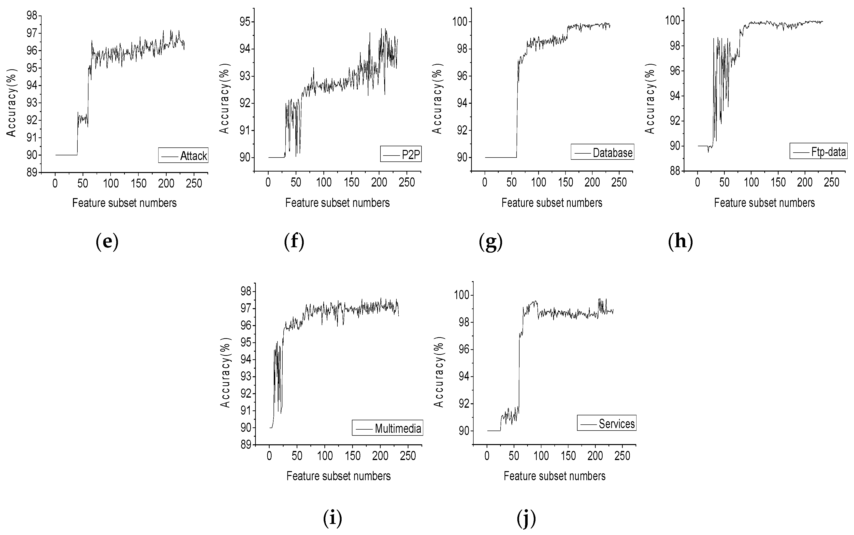
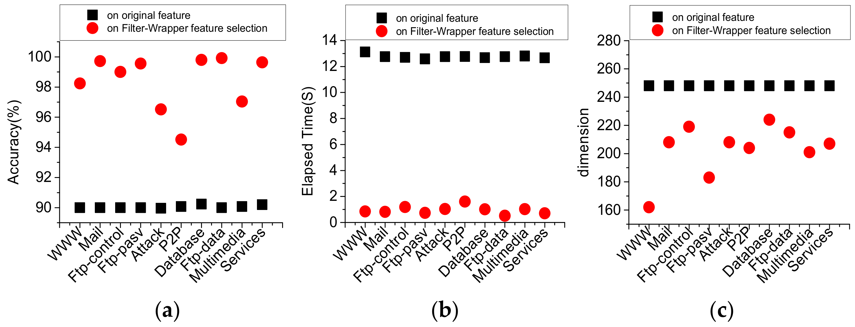
4.2. Performance Analysis of Filter-Wrapper Feature Selection

The original dimensionality is 248-dimensional, so the dimension is still high. These high-dimensional features will increase the computational complexity and the training time of the SVM classifier. The filter-wrapper hybrid feature selection model proposed in this section adopts Filter information gain (IG) algorithm to remove features whose weights are less than the set threshold $\delta \left(\delta =0\right)$ from the original data set to obtain a new feature subset. Based on the IG of the feature subset selection, wrapper is adopted based on the SVM classifier, and heuristic forward search strategy is used to select second-feature, which reduces the feature dimension and improves the performance of SVM classification.

Based on the filter IG algorithm, the individual feature is analyzed, and the contribution of each feature to the classification is investigated. The features whose weights are less than the threshold are deleted. The feature numbers and feature descriptions are shown in Table 2. A new feature subset is formed after the feature with weight 0 is deleted. Based on the SVM classifier, the wrapper second-feature selection is carried out by a backward search strategy on this feature subset.

Table 2. Features of weights less than $\delta \left(\delta =0\right)$ deleted based on Information Gain.

Feature Number	Feature Description	Feature Number	Feature Description
40	dsack_pkts_sent_b a	78	urgent_data_bytes_b a
53	zwnd_probe_pkts_a b	92	zero_win_adv_b a
54	zwnd_probe_pkts_b a	102	missed_data_b a
55	zwnd_probe_pkts_b a	103	truncated_data_a b
56	zwnd_probe_bytes_b a	104	truncated_data_b a
75	urgent_data_pkts_a b	105	truncated_packets_a b
76	urgent_data_pkts_b a	106	truncated_packets_b a
77	urgent_data_bytes_a b

Figure 5 shows the classification accuracy of each network traffic increasing with the feature number of the new feature subset. According to the graph, we can select the feature subset with the highest contribution of the combined feature corresponding to each flow. The feature number and classification accuracy of the feature subset based on filter-wrapper feature selection are shown in Table 3.

Figure 5. The accuracy of Traffic Classification corresponding to feature subsets.(a) www; (b) Mail; (c) Ftp-control; (d) Ftp-pasv; (e) Attack; (f) P2P; (g) Database; (h) Ftp-data; (i) Multimedia; (j) Services.

Table 3. Feature subset and accuracy based on Filter-Wrapper feature selection.

Traffic Class	The Number of Optimal Feature Combinations	Accuracy (%)
WWW	162	98.8
Mail	208	99.96
FTP-control	219	99.44
FTPp-pasv	183	99.8
Attack	208	97.2
P2P	204	94.76
Database	224	99.96
FTP-data	215	99.98
Multimedia	201	97.64
Services	207	99.76

In order to investigate whether the method can achieve the same classification effect based on smaller training samples, 5000 samples are randomly selected, and the classification accuracy is obtained based on the feature dimension of the Filter-Wrapper feature selection. The feature dimension, classification accuracy, execution time of the method are compared with the classification effect of SVM in the original feature set as shown in Figure 6.

Figure 6. Comparison of classification performance before and after Filter-Wrapper feature selection. (a) Accuracy (%); (b) Elapsed time (s); (c) Dimensions.

It can be seen from the diagram that the classification effect of SVM is improved obviously after the process of feature selection based on the filter-wrapper model. The accuracy of traffic classification: WWW is 98.24%, mail is 99.72%, FTP-control is 99%, FTP-pasv is 99.56%, P2P is 94.52%, database is 99.8%, FTP data is 99.92%, multimedia is 97.04%, and services is 99.64%. The execution times of each type of traffic are: WWW 0.85 s, mail 0.82 s, FTP-control 1.18 s, FTP-pasv 0.73 s, attack, 1.03 s, P2P 1.6 s, database 1.01 s, FTP-data, 0.51 s, multimedia 1.03 s, services 0.7 s. The average classification accuracy is 8.34% higher than that before feature selection, the average feature dimension is 18.15% lower, and the execution time is 92.5% shorter than that before feature selection.

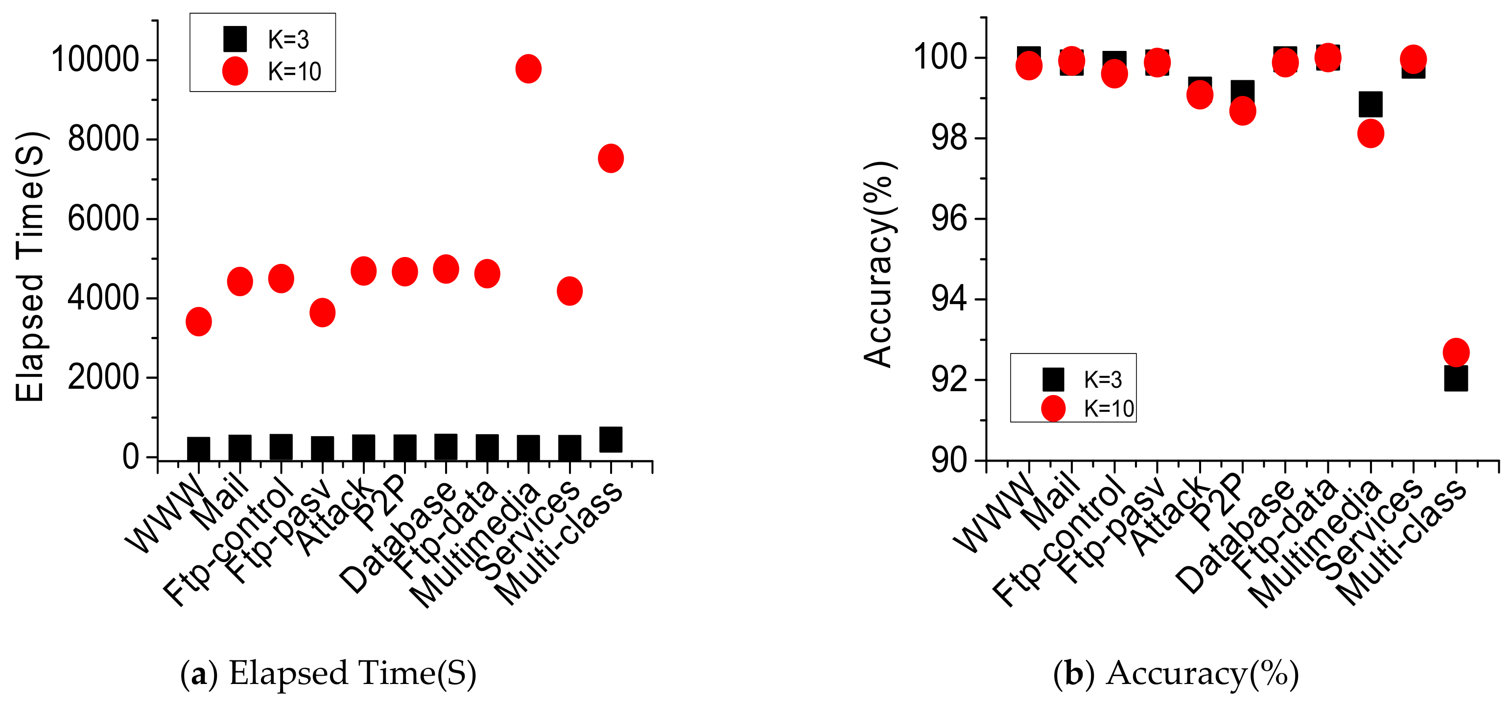
4.3. Performance Analysis of Parameter Optimization for Improved Grid Algorithm

4.3.1. Initialization Parameter Setting

After adopting the filter-wrapper feature selection, the average two-classification performance is better, but the classification accuracy of P2P has not reached 95%. In addition, the multi-classification performance is not ideal. The optimal feature subset dimension is 219, and the classification accuracy is 82.6%. Therefore, the improved grid search algorithm (IGS) is used to optimize the parameters and the SVM classification model is further optimized. The initial search range of the penalty parameter C of IGS is $\left[2^{-10},2^{10}\right]$, the initial search range of the parameter $\gamma$ of RBF kernel function is $\left[2^{-10},2^{10}\right]$, and the search step is increased to 1.5 times the default step size. The k–CV method is used to test the training set $\left(k=3\right)$, to optimize the parameters combination $\left(C,\gamma \right)$. The k value k–CV affects the classification accuracy and computational complexity. k = 3 and k = 10 are compared experimentally, as shown in Figure 7. The execution time k = 3 is significantly shorter than that of k = 10. The average execution time of two-classification is shortened 95.25% and the execution time of multi-classification is shortened 94.22%. Between the two test sets (k = 3, k = 10), the accuracy of two-classification is less than 0.2% and the accuracy of multi-classification is less than 0.7%. As a result, the experiment adopts k = 3(3-CV) to optimize the parameter combination $\left(C,\gamma \right)$, which can reduce the computational complexity while avoiding overfitting and underfitting.

Figure 7. Comparison of performance between two-Classification and multi-Classification under different $k-CV\left(k=3,k=10\right)$. (a) Elapsed Time (S); (b) Accuracy (%).

4.3.2. Initial Grid Parameter Optimization

After the initial parameter optimization, the combination C of the penalty parameter of SVM, the parameter $\gamma$ of RBF kernel function and the accuracy of the classification of the test set are shown in Table 4. From the table, we can see that the average accuracy of SVM two-classification is 99.648% after the initial parameter optimization of IGS, and the accuracy of multi-classification is 92.04%, which is 9.44% higher than the traditional SVM classification. However, the value of penalty parameters C for initial optimization of individual traffic is too large, such as P2P and Multimedia traffic’s C value is more than 700. The larger the value C is, the greater the penalty for empirical error is, the greater the complexity of the learning machine is and the smaller the value of empirical risk is, which will result in over-fitting and it can lead to the deterioration of the generalization ability of SVM. For this situation, IGS performs second-optimization.

Table 4. Optimal $\left(C,\gamma \right)$ after initial search of IGS and classification performance of the test set.

Traffic Class	The Number of Optimal Feature Combinations	$\mathit{C}$	$\mathit{\gamma }$	Accuracy (%)
WWW	162	11.3137	0.0625	99.96
Mail	208	0.5	0.0220971	99.88
Ftp-control	219	32	0.00276214	99.84
Ftp-pasv	183	11.3137	0.0220971	99.88
Attack	208	90.5097	0.0220971	99.20
P2P	204	724.077	0.0625	99.12
Database	224	4	0.0220971	99.96
Ftp-data	215	1.41421	0.0220971	100.00
Multimedia	201	724.077	0.0078125	98.84
Services	207	4	0.5	99.80
Multi-class	219	11.3137	0.0220971	92.04

4.3.3. Second-Grid Parameter Optimization

The IGS algorithm judges the penalty parameter C in the process of second-grid parameter optimization. When C does not exceed the threshold $\delta \left(\delta =100\right)$, according to the contour map of the initial parameter optimization, the searching range is reduced according to the highest accuracy area. In the second-search process, the step size is reduced to 0.5 times of the default step size, so that the IGS carries out the second fine search in the ideal region. When C exceeds the threshold value $\delta \left(\delta =100\right)$, using the contour map optimized by reference to the initial parameters, the method of opposite direction grid search from the highest accuracy region to the lower accuracy region is used. Until $C$ reaches the threshold value which satisfies the condition $\left(C\le 100\right)$, thus it avoids the over-fitting and enhances the SVM classification generalization ability. The optimal parameter combination $\left(C,\gamma \right)$ values are shown in Table 5. You can see that the penalty parameters C in the SVM classification model and the parameters $\gamma$ of the RBF kernel function are within the threshold constraint range and they are the optimal parameters after the second-parameter optimization of the IGS.

Table 5. The best parameters combination of $\left(C,\gamma \right)$ after the second-parameter optimization of the IGS.

Traffic Class	$\mathit{C}$	$\mathit{\gamma }$	Traffic Class	$\mathit{C}$	$\mathit{\gamma }$
WWW	1.41421	0.176777	Database	2	0.0110485
Mail	1	0.125	Ftp-data	1	0.03125
Ftp-control	1.41421	0.0220971	Multimedia	22.6274	0.015625
Ftp-pasv	5.65685	0.0625	Services	4	0.0883883
Attack	8	0.03125	Multi-class	5.65685	0.03125
P2P	32	0.015625

4.4. Performance Comparison

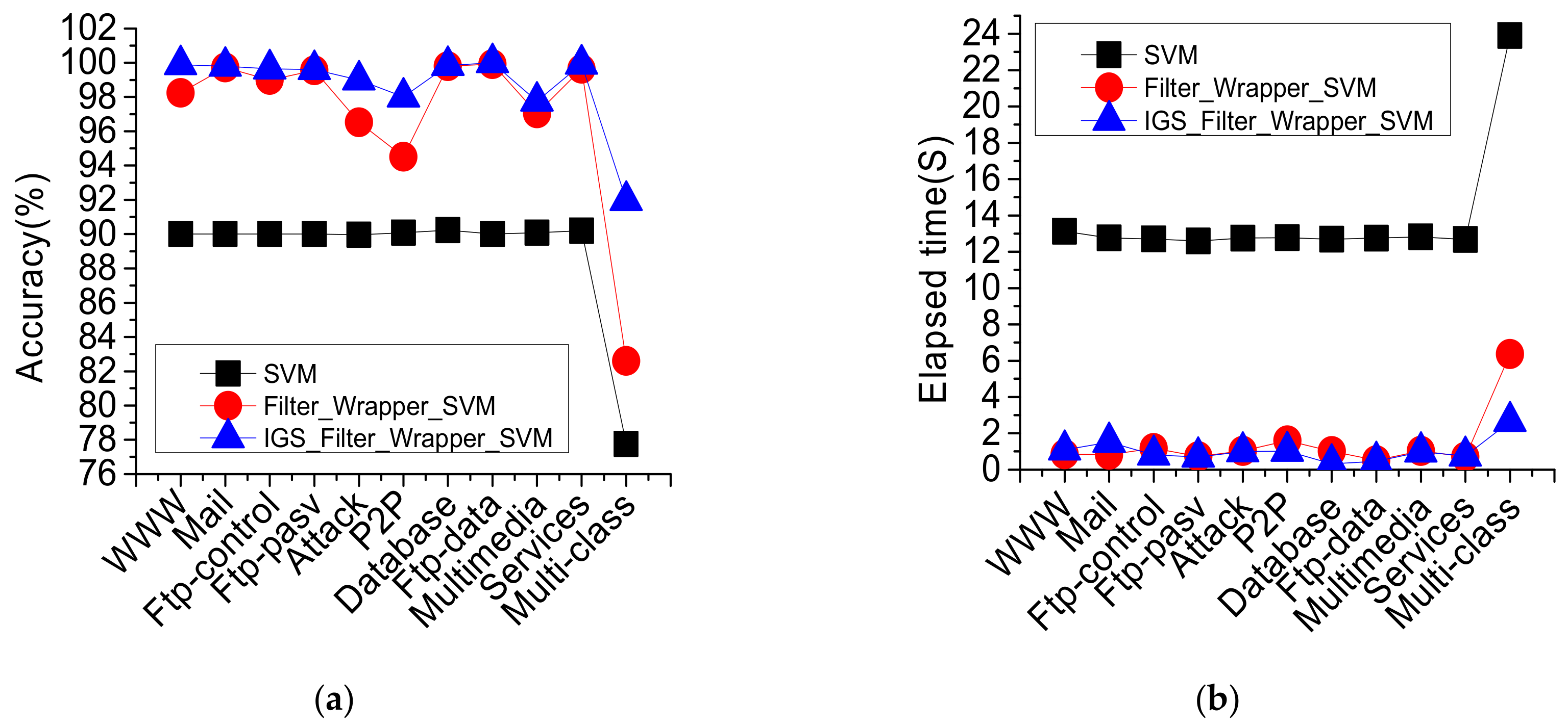
4.4.1. Comparison and Analysis of Each Stage of the IGS Algorithm

The improved IGS is based on the proposed feature selection method to further optimize the working parameters of SVM, thus to improve the classification performance and generalization ability of SVM. Therefore, we compare the feature dimension selection and parameter optimization at each stage. In Figure 8, we compare the two-classification and multi-classification performance of the SVM model in the original, dimension selection and parameter optimization stages.

Figure 8. Performance comparison of SVM two-Classification and multi-Classification before and after IGS. (a) Accuracy (%); (b) Elapsed time (S).

Through comparison and analysis, the average accuracy of the two-classification of the IGS_filter-wrapper_SVM model reached 99.34%, which is 9.28% higher than the original SVM. The average accuracy of the multi-classification of the IGS_filter-wrapper_SVM model reached 91.96%, which is 14.2% higher than the original SVM, and the average feature dimension is 18.15% lower. Based on the proposed feature selection model, the classification performance of SVM is improved greatly after the parameters optimization of IGS. Although the IGS_filter-wrapper_SVM model takes a certain amount of learning time before classification, the first average learning time is 8.97 min, but once the feature and classifier parameters are selected, the classification model can achieve accurate and fast classification later. The model two-classification is 93.19% shorter on average execution times, and its multi-classification is 88.87% shorter on average execution times. In addition, due to the second-optimization of SVM working parameters by IGS, the threshold of parameter range is constrained, which avoids overfitting and improves the generalization ability of SVM.

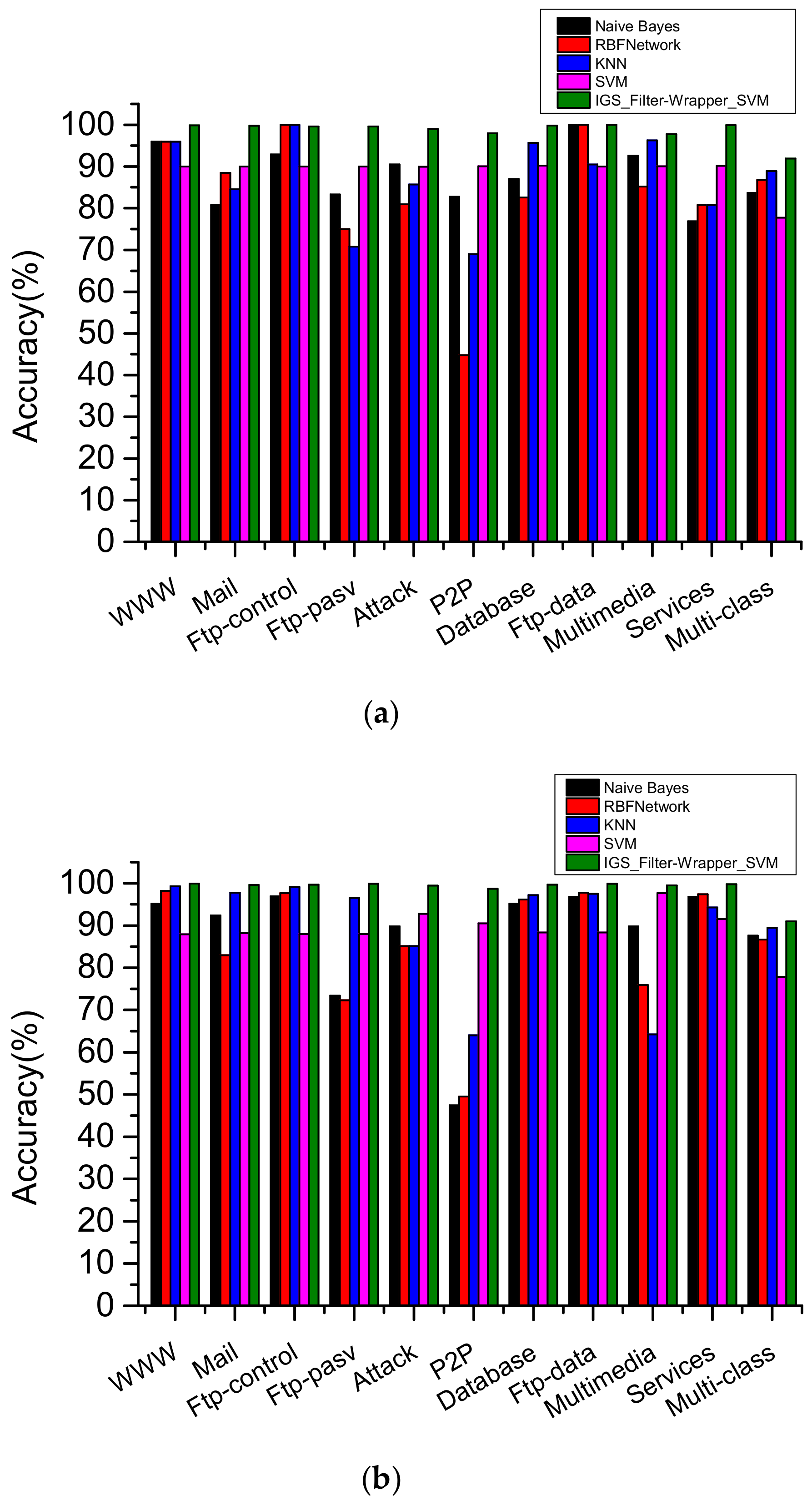
4.4.2. Comparison and Analysis of IGS and Other Algorithms

The improved SVM classification model, IGS_filter-wrapper_SVM, is compared with other typical supervised classification algorithms, naive Bayes, RBFNetwork, KNN, and the original SVM. The results are shown in Figure 9.

Figure 9. Comparison of five algorithms on data sets with different sample sizes. (a) Accuracy (%) (sample size = 5000); (b) Accuracy (%) (sample size = 24897).

The average classification accuracy of IGS_filter-wrapper_SVM was 99.34%, 11.06% higher than that of naive Bayes, 16% higher than RBFNetwork, 12.4% higher than KNN, 9.28% higher than the original SVM. The accuracy of multi-classification reached 91.96%, 8.24% higher than naive Bayes, 5.16% higher than RBFNetwork, 3.06% higher than KNN, 14.22% higher than original SVM.

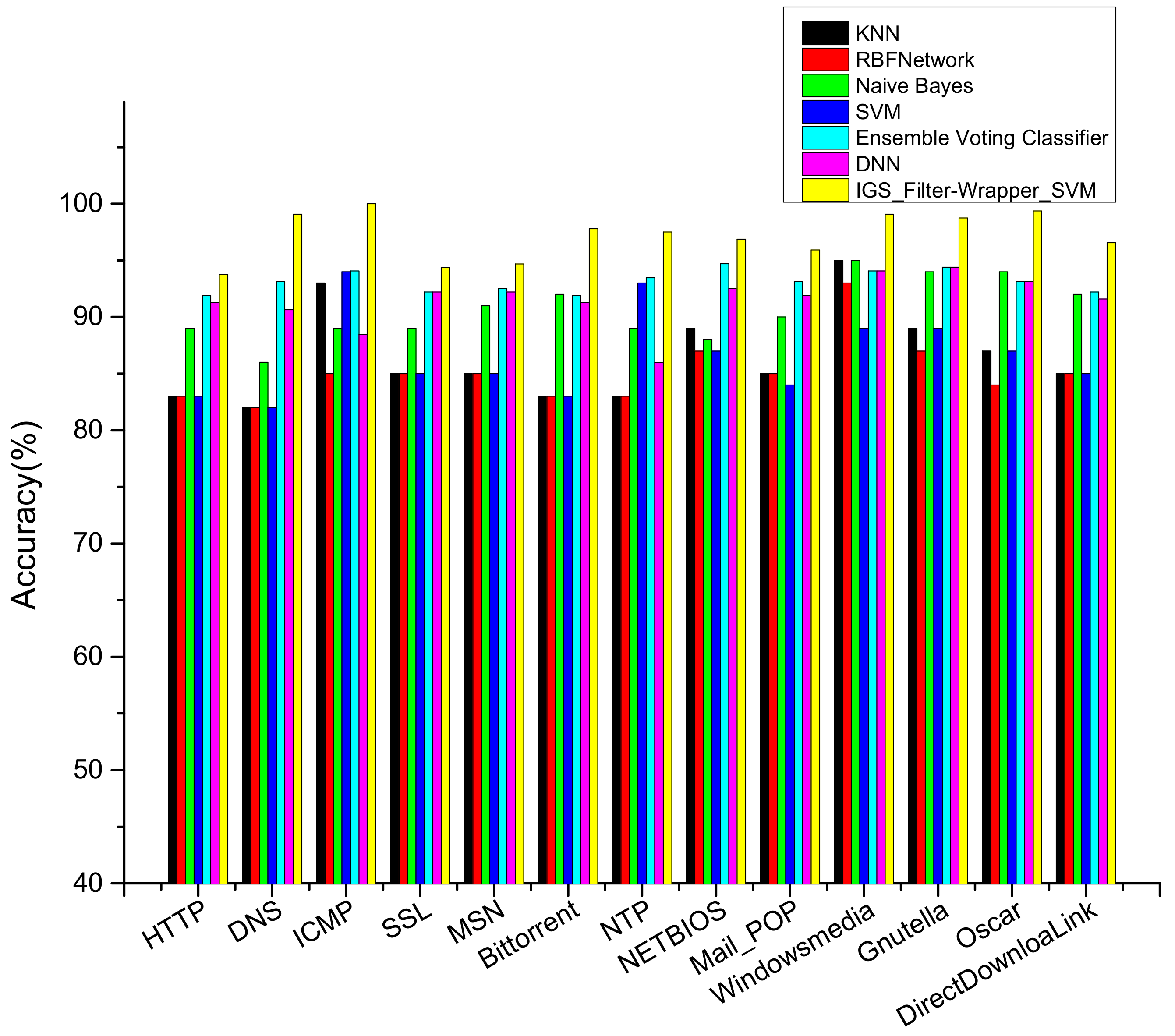
4.4.3. Comparison and Analysis of IGS on CAIDA Datasets

In order to verify the universality of IGS_filter-wrapper_SVM, we also inspect the classification performance of it on the CAIDA dataset [32]. The CAIDA was collected from a different period in 3 days. The dataset includes traffic logs, topology logs, traffic summary statistics, security logs, worm traffic, and other applications, which is shown in Table 6.

Table 6. CAIDA Dataset.

Traffic Class	Sample Number	Traffic Class	Sample Number
Http	33667	NETBIOS	58
DNS	22814	Mail_POP	64
ICMP	1318	Windows media	46
SSL	2671	Gnutella	108
MSN	190	Oscar	126
Bittorrent	61	DirectDownloadLink	45
NTP	81

In order to reduce the imbalance of the data, we deleted the traffic flows in which the samples are very few, and we extracted samples randomly from every subset to build the unbiased new training dataset. 50% of the sample data are used as the training set, and the others are used as the test set. The classification result is shown in Figure 10.

Figure 10. Comparison of different algorithms on the CAIDA dataset.

As is shown in Figure 10, the average classification accuracy of the IGS_filter-wrapper_SVM is 97.2%, 10.8% higher than KNN, 12.1% higher than RBF network, 6.6% higher than naive Bayes, 4% higher than ensemble voting classifier, 5.7% higher than DNN, and 10.6% higher than traditional SVM. The result showed that the IGS_filter-wrapper_SVM is appropriate for the CAIDA dataset. In addition, with the filter-wrapper feature selection and the IGS parameter optimization algorithms, the training time consumption reduced from 3.12S to 0.31 s, which reduced the model computation complexity obviously.

4.4.4. Comparison of IGS and Other Related Approaches

In order to verify the overall performance of the IGS_filter-wrapper_SVM model, we compare the model with other related approaches. Three properties are compared in Table 7, they are feature selection, parameter optimization, and accuracy performance. From the analysis in Table 7, the accuracy of the IGS_filter-wrapper_SVM model is the highest. References [15,16] select features depending on experience or manual tuning, which reduces the performance of classification. In [17], the deep learning model learns features automatically from all data, and it does not consider excluding irrelevant features, in which the noise features may increase the risk of overfitting. The filter-wrapper feature selection method selects the key feature combinations accurately and avoids the false deletion of combined features, which achieves the effect of reducing the dimension and shortening the training time. The parameter optimization is used in reference [21,33], and it is the original grid search method which brings a higher risk of overfitting. The back-propagation algorithm in [17] is a kind of local search algorithm, which may fall into a local optimum solution. The IGS method proposed in this paper can convergence to a globally optimal solution, and doesn’t need to search widely. From this perspective, the IGS_filter-wrapper_SVM model is more effective.

Table 7. Related approaches.

Algorithm	Feature Selection	Parameters Optimization	Classification Accuracy
IGS_filter-wrapper_SVM	Filter-Wrapper	IGS	more than 99.34%
Ensemble learning [15]	Identification Engineer	no	more than 99%
Ensemble learning [16]	Burst Threshold	no	more than 80%
Deep learning [17]	No	Back-Propagation	more than 80%
SVM [21]	Sequential forward	Grid-Search	97.17%
SVM [33]	No	Grid-Search	more than 95%

5. Conclusions

In the process of network traffic classification, the filter-wrapper hybrid feature selection model is proposed to solve the problem that high dimensional data leads to the increase of time and space complexity of SVM. The model can solve the problem that interferences between features lead to the degradation of the classification performance. In addition, an improved grid search parameter optimization algorithm(IGS), is proposed to find a set of optimal parameter combinations for model training, which can dynamically adjust the second search region, reduce the density of second grid generation and improve the search efficiency of the algorithm. At the same time, the overfitting in the optimization process is prevented, and the generalization ability of SVM is improved. The experimental results of real data sets show that the combined optimization network traffic classification model proposed in this paper has an obvious dimensionality reduction effect, and the optimal parameter combination can be found in the parameter space at a finite computational cost. The classification and generalization ability of SVM is increased effectively and the classification effect is very close to the original sample data set under the small unbiased training sample. It has practical significance for real-time classification of network traffic. It provides the basis for real-time dynamic monitoring of network traffic, user behavior mining, and identification of network attacks.

In addition, the proposed method of this paper can realize the differential management of the corresponding network traffic, and provide a solid foundation and basis for the subsequent network protocol design, network operation management, network traffic scheduling. It can also be extended in network traffic abnormal pattern recognition, mobile encryption traffic pattern recognition and so on.

References

1. Max, B.; Mritunjay, K. Identifying P2P traffic: A survey. Peer Peer Netw. Appl. 2017, 10, 1182–1203. [Google Scholar]
2. Yinxiang, H.; Yun, L.; Baohua, Q. Internet traffic classification based on Min-Max Ensemble Feature Selection. In Proceedings of the 2016 International Joint Conference on Neural Networks (IJCNN), Vancouver, BC, Canada, 24–29 July 2016. [Google Scholar]
3. Hongtao, S.; Gang, L.; Hai, W. A novel traffic identification approach based on multifractal analysis and combined neural network. Ann. Telecommun. 2014, 69, 155–169. [Google Scholar]
4. Neeraj, N.; Shikha, A.; Sanjay, S. Recent Advancement in Machine Learning Based Internet Traffic Classification. J. Procs. 2015, 60, 784–791. [Google Scholar]
5. Yu, W.; Yang, X.; Wang, Z.; Shunzheng, Z. Generating regular expression signatures for network traffic classification in trusted network management. J. Netw. Comput. Appl. 2012, 35, 992–1000. [Google Scholar]
6. Alok, T.; Ruben, T.; Marios, I.; Ram, K.; Antonio, N. Towards self adaptive network traffic classification. Comput. Commun. 2015, 56, 35–46. [Google Scholar]
7. Hongtao, S.; Hongping, L.; Dan, Z.; Chaqiu, C.; Wei, W. Efficient and robust feature extraction and selection for traffic classification. Comput. Netw. 2017, 119, 1–16. [Google Scholar]
8. Neminath, H.; Mayank, S. $BitCoding$: Network Traffic Classification through Encoded Bit Level Signatures. IEEE/ACM Trans. Netw. 2018, 26, 2334–2346. [Google Scholar]
9. Jun, Z.; Chao, C.; Yang, X.; Wanlei, Z.; Athanasios, V.V. An Effective Network Traffic Classification Method with Unknown Flow Detection. IEEE Trans. Netw. Serv. Manage. 2013, 10, 133–147. [Google Scholar]
10. Iliofotou, M.; Pappu, P.; Faloutsos, M. Network Traffic Analysis Using Traffic Dispersion Graphs (TDGs): Techniques and Hardware Implementation; Technical Report; University of California: Riverside, CA, USA, 2007. [Google Scholar]
11. Bonfiglio, D.; Mellia, M.; Meo, M.; Rossi, D. Detailed analysis of skype traffic. IEEE Trans. Multimedia 2008, 11, 117–127. [Google Scholar] [CrossRef]
12. Margaret, G.; Darshan, B.; Michel, C.; Josiah, D. Identifying infected users via network traffic. Comput. Secur. 2019, 80, 306–316. [Google Scholar]
13. Zhihong, R.; Weina, N.; Xiaosong, Z.; Hongwei, L. Tor anonymous traffic identification based on gravitational clustering. Peer Peer Netw. Appl. 2018, 11, 592–601. [Google Scholar]
14. Songyin, L.; Jing, H.; Shengnan, H.; Tiecheng, S. Improved EM method for internet traffic classification. In Proceedings of the 2016 8th International Conference on Knowledge and Smart Technology (KST), Chiangmai, Thailand, 3–6 February 2016; pp. 13–17. [Google Scholar]
15. Dainotti, A.; Gargiulo, F.; Kuncheva, L.I. Identification of traffic flows hiding behind TCP port 80. In Proceedings of the 2010 IEEE International Conference on Communications, Cape Town, South Africa, 23–27 May 2010; pp. 1–6. [Google Scholar]
16. Aceto, G.; Ciuonzo, D.; Montieri, A. Multi-classification approaches for classifying mobile app traffic. J. Netw. Comput. Appl. 2018, 103, 131–145. [Google Scholar] [CrossRef]
17. Aceto, G.; Ciuonzo, D.; Montieri, A. Mobile encrypted traffic classification using deep learning. In Proceedings of the 2018 Network Traffic Measurement and Analysis Conference (TMA), Vienna, Austria, 26–29 June 2018; pp. 1–8. [Google Scholar]
18. Wang, P.; Chen, X.; Ye, F.; Sun, Z. A survey of techniques for mobile service encrypted traffic classification using deep learning. IEEE Access 2019, 7, 54024–54033. [Google Scholar] [CrossRef]
19. Vijayanand, R.; Devaraj, D.; Kannapiran, B. Intrusion detection system for wireless mesh network using multiple support vector machine classifiers with genetic-algorithm-based feature selection. Comput. Secur. 2018, 77, 304–314. [Google Scholar] [CrossRef]
20. Alice, E.; Francesco, G.; Luca, S. Support Vector Machines for TCP traffic classification. Comput. Netw. 2009, 53, 2476–2490. [Google Scholar]
21. Yuan, R.; Li, Z.; Guan, X.; Xu, L. An SVM-based machine learning method for accurate internet traffic classification. Inf. Syst. Front. 2010, 12, 149–156. [Google Scholar] [CrossRef]
22. Sicker, D.C.; Ohm, P.; Grunwald, D. Legal issues surrounding monitoring during network research. In Proceedings of the 7th ACM SIGCOMM Conference On Internet Measurement, San Diego, CA, USA, 24–26 October 2007; pp. 141–148. [Google Scholar] [CrossRef]
23. Scott, D.; Stuart, R. NP-Completeness of Searches for Smallest Possible Feature Sets; AAAI Press: Palo Alto, CA, USA, 1994; pp. 37–39. [Google Scholar]
24. Selvi, S.; Manimegalai, D. Task Scheduling Using Two-Phase Variable Neighborhood Search Algorithm on Heterogeneous Computing and Grid Environments. Arab. J. Sci. Eng. 2015, 40, 817–844. [Google Scholar] [CrossRef]
25. Adriana, M.C. Tuning model parameters through a Genetic Algorithm approach. In Proceedings of the 2016 IEEE 12th International Conference on Intelligent Computer Communication and Processing (ICCP), Cluj-Napoca, Romania, 8–10 September 2016; pp. 135–140. [Google Scholar]
26. Di, H.; Yunlv, H. An Improved Tabu Search Algorithm Based on Grid Search Used in the Antenna Parameters Optimization. Math. Probl. Eng. 2015. [Google Scholar] [CrossRef]
27. Yudong, Z.; Zhangjing, Y.; Huimin, L.; Xingxing, Z.; Preetha, P.; Qingming, L.; Shuihua, W. Facial Emotion Recognition Based on Biorthogonal Wavelet Entropy, Fuzzy Support Vector Machine, and Stratified Cross Validation. IEEE Access 2015, 4, 8375–8385. [Google Scholar]
28. Lei, M.; Manchun, L.; Yu, G.; Tan, C.; Xiaoxue, M.; Lean, Q. A Novel Wrapper Approach for Feature Selection in Object-Based Image Classification Using Polygon-Based Cross-Validation. IEEE Geosci. Remote. Sens. Lett. 2017, 14, 409–413. [Google Scholar]
29. Moore, A.; Zuev, D. Discriminators for Use in Flow-Based Classification; Intel Research: Cambridge, UK, 2005. [Google Scholar]
30. Mashael, A.; Kevin, B.; Ian, G. Enhancing Tor’s performance using real-time traffic classification. In Proceedings of the 2012 ACM conference on Computer and communications security, Raleigh, CA, USA, 16–18 October 2012; pp. 73–84. [Google Scholar]
31. Chihchung, C.; Chihjen, L. LIBSVM: A library for support vector machines. ACM Trans. Intell. Syst. Technol. 2011, 2, 1–27. [Google Scholar]
32. The Cooperative Association for Internet Data Analysis (CAIDA). Available online: http://www.caida.org (accessed on 1 September 2012).
33. Sena, G.; Pablo, B. Statistical traffic classification by boosting support vector machines. In Proceedings of the 7th Latin American Networking Conference, New York, NY, USA, 4–5 October 2012. [Google Scholar]
Article Metrics
Citations
Article Access Statistics
Multiple requests from the same IP address are counted as one view.