Abstract
Focusing on ill-structured multiple attribute decision-making (MADM) problems, including decision hesitancy and attribute prioritization relationships, this paper investigates appropriate approaches for decision making. Firstly, we introduce the probabilistic hybrid linguistic term set (P-HLTS) for capturing probabilistic preferences about possible linguistic labels belonging to a wide range of hesitant linguistic term sets. Entropy and distance measurements for P-HLTS are developed without arbitrary complementing operations. To facilitate decision making with attribute prioritization relationships, we present a probabilistic uncertain balanced linguistic-prioritized weighted average (PUBL-PWA) operator and the probabilistic uncertain balanced linguistic-induced prioritized ordered weighted average (PUBL-IPOWA) operator. In terms of the strength of the above tools, we further construct two multiple attribute group decision-making (MAGDM) approaches under P-HLTS environments, namely, an approach for decision-making situations where attribute prioritization relationships are known in advance and the relative importance of decision makers (DMs) or decision-making units (DMUs) is not required for consideration, and second approach for decision-making situations where both attribute prioritization relationships and the weighted vectors of DMs or DMUs are explicitly unknown. In general, our proposed approaches are more flexible and practical when considering heterogeneous opinions, avoiding information distortion brought about by complementing operation-based distance measures. Furthermore, illustrative application studies are conducted to verify our developed approaches.
1. Introduction
Multiple attribute decision-making (MADM) theory is an indispensable part of decision analysis theory, [1] and has been successfully applied to practical problems in many fields [2,3,4,5,6,7,8]. The main purpose of MADM is to find desirable solutions from finite alternatives according to assessments under a set of attributes. Due to increasing complexity and uncertainty in socioeconomic decision-making environments, single decision makers usually become less competent in evaluating all aspects of complicated decision-making problems [9,10]. Multiple attribute group decision-making (MAGDM) approaches thus have been developed by extending MADM to group settings, where a number of decision makers (DMs) or decision-making units (DMUs) are invited to present their assessments [5,11,12]. To deal with the uncertainty in decision maker preferences [13,14,15,16,17], fuzzy set theory [18] and its extensions have been introduced to enhance conventional MAGDM models, such as intuitionistic fuzzy sets [19,20], hesitant fuzzy sets [21], dual hesitant fuzzy sets [22], interval-valued dual hesitant fuzzy sets [23], and probabilistic dual hesitant fuzzy sets [24], among others.
However, when it comes to more complicated MAGDM problems, where problem structures are ill-defined for fuzzy quantification, Zadeh [25] has advocated the usage of linguistic variables for decision makers to qualitatively express their uncertain preferences. To this end, because of the merit in eliciting decision maker assessments more directly and precisely, linguistic variables have been continuously extended to accommodate various scenarios, such as unbalanced linguistic variables [26,27,28,29], uncertain linguistic variables [30,31,32,33], intuitionistic uncertain variables [34,35], hesitant fuzzy uncertain linguistic variables [15], and hesitant fuzzy unbalanced linguistic variables [36], among others. Although the above extensions of linguistic variables are very effective in situations where decision makers can approximate the most precise linguistic label in accordance with their assessment, Rodríguez et al. [37] revealed that decision makers are often cognitively irresolute among several possible linguistic labels. Taking this a step further, Pang et al. [11] and Liao et al. [38] point out the phenomena that DMs or DMUs usually will have different importance degrees in terms of those possible linguistic labels. Pang et al. [11] thus introduced the probabilistic linguistic term set (PLTS), which is capable of dealing with situations where probabilistic distributions cannot be acquired completely in reality, and is capable of carrying out probability information aggregation without a loss of information [24]. Since its introduction, PLTS has been successfully applied to solve practical MADM problems in various settings [38,39,40,41,42,43,44,45,46]. As can be seen, these studies all only allow decision makers to depict their cognitive models through balanced linguistic terms sets (BLTS) [25] which are uniformly and symmetrically distributed. However, field investigations [26,28] have revealed that decision makers usually tend to utilize nonuniform or asymmetrical linguistic term sets, referred to as unbalanced linguistic term sets (UBLTSs) [27], for expressing their assessments appropriately and flexibly. Additionally, when trying to obtain linguistic expressions that closely follow decision maker cognitive models, Rodríguez et al. [47] and Wang [48] have advocated for the adoption of consecutive and nonconsecutive comparative linguistic expressions. Therefore, in order to address different cognitive models where DMs or DMUs hold real problems, in this paper, we propose an effective expression tool for probabilistic hybrid linguistic term sets (P-HLTSs). P-HLTSs manage to enhance classical PLTS by accommodating a wide range of linguistic expression forms when considering diverse cognitive models, including balanced linguistic sets, unbalanced linguistic term sets, uncertain unbalanced linguistic term sets, comparative balanced linguistic term sets, and comparative unbalanced linguistic term sets. Comparatively, P-HLTS thus behaves in a more flexible and practical manner.
With respect to complicated decision-making situations which require decision information in the form of PLTS, pioneering efforts have been accumulatively paid to various effective MADM methodologies, such as that of Pang et al. [11], who introduced an extended TOPSIS-based MAGDM approach by use of proposed fundamental probabilistic linguistic averaging operators. Liu and Fei [49] developed two multiple attribute decision-making methods based on their probabilistic linguistic Archimedean Muirhead mean aggregation operators [49]. Liu and Li [50] designed an effective MAGDM approach to consider interrelationships among input arguments by use of generalized Maclaurin symmetric mean operators. Lin et al. [51] extended PLTS to define the probabilistic uncertain linguistic term set (PULTS) and devised a TOPSIS-based MAGDM method with the support of aggregation operators for PULTS. Liu et al. [40] developed an approach where attributes’ weights were derived by their defined entropy measures for PLTS. Wu and Liao [41] studied a novel group decision-making approach based on ORESTE methods and PLTS under a QRD framework for design selection problems. Xiang et al. [42] studied an interactive venture capital group decision-making approach under the PLTS scenario, in which interactions among venture capitalists and entrepreneurs were considered to dynamically deduce weight information. To deal with emergency decision-making problems, Gao et al. [43] developed an approach using probabilistic linguistic preference relations (PLPRs), where they equally synthesized subjective possibilities given by decision makers and objective possibilities which were obtained by case-based reasoning. Liao et al. [38] proposed an LINMAP-based group decision-making method where the developed linear programming models were used to calculate the weights of evaluative attributes. Some other classical decision-making methodologies have also been extended to PLTS environments, such as the probabilistic linguistic TODIM method [45] and the probabilistic linguistic VIKOR method [46]. However, to the best of our knowledge, the approaches in the literature are incapable of addressing the special type of decision-making problems which exist where decision information about attributes’ prioritization relationships is unavailable. In fact, the phenomena of prioritization relationships is quite common when making decisions, due to limited knowledge or problematic complexity, presenting difficulties or unwillingness to provide complicated preference relationships, as required in AHP-like analytical models, while they are quite sure about the existence of prioritization relationships among evaluative attributes [52,53,54,55,56,57,58]. Therefore, to tackle ill-structured, complicated decision-making problems where attribute prioritization relationships exists, it is indispensable to study effective approaches that are simultaneously capable of taking the strength of PLTS and exploiting decision information denoted by attributes’ prioritization relationships.
To do so, we firstly employ the newly defined probabilistic hybrid linguistic term set (P-HLTS) to empower DMs or DMUs in choosing the most appropriate linguistic term set for depicting their preferences. Secondly, in the light of Yager’s [52,53] prioritized average (PA) operator theory, which manages to concurrently consider assessments under evaluative attributes and considering prioritization relationships among the attributes, we develop two prioritized average operators for MADM under P-HLTS environments, namely, the probabilistic uncertain balanced linguistic-prioritized weighted average (PUBL-PWA) operator and the probabilistic uncertain balanced linguistic-induced prioritized ordered weighted average (PUBL-IPOWA) operator. Further, based on the defined operational rules and the entropy measure of P-HLTS and the PUBL-PWA operator, we construct a MAGDM approach to solve decision-making problems where attributes’ prioritization relationships have been determined in advance, and the relative importance of DMs or DMUs does not require consideration. Furthermore, to tackle more complicated decision-making problems, where attributes’ prioritization relationships and weighting vectors for DMs or DMUs are both explicitly unknown, we utilize the PUBL-IPOWA operator to construct another MAGDM approach, in which we introduce a distance measure for P-HLTS to develop a divergence measure-based method for obtaining the unknown attributes’ prioritization relationships and a similarity degree-based method for deriving weighting vectors for DMs or DMUs.
The content of this paper is organized as follows: In Section 2, we briefly introduce some preliminary information about probabilistic linguistic term sets (PLTSs) [11]. In Section 3, we firstly propose the concept of probabilistic hybrid linguistic term sets (P-HLTSs) and define some fundamental operational rules for P-HLTSs, then, a distance measure and entropy measure are both developed for P-HLTSs. In Section 4, we define the PUBL-PWA and PUBL-IPOWA operators. Their desirable properties are also studied. Subsequently, in Section 5, the details of the first and second approaches are presented. Next, we conduct a case study in order to verify the two approaches, considering an evaluation of the usability of a governmental website in Section 6. Finally, our conclusions are presented in Section 7.
2. Preliminaries
2.1. Probabilistic Hesitant Fuzzy Set (P-HFS)
Definition 1.
[59] If we letbe a finite set, then a probabilistic hesitant fuzzy set (P-HFS) onis defined as follows:
whererepresents the membership degreeassociated with the probability,is the probabilistic hesitant fuzzy element (P-HFE), andis the number of all different membership degrees in.
2.2. Probabilistic Linguistic Term Set (PLTS)
In practice, decision makers may always have hesitancy among several possible linguistic terms when expressing their preferences, and the complete probabilistic distribution of these linguistic terms is usually not easily obtained accurately [24]. Pang et al. [11] thus have proposed the concept of a probabilistic linguistic term set (PLTS), which extends the hesitant fuzzy linguistic term set (HFLTS) [37] by adding probability information, without loss of any original compound decision information.
Definition 2.
[11] If we letbe a definite linguistic term set (LTS), a PLTS is defined as follows:
whereis the linguistic termassociated with the probabilityandis the number of all different linguistic terms in.
In the equation above, if , then we have the complete information of the probabilistic distribution of all terms, whereas if , partial ignorance exists, because current knowledge is not enough to provide complete assessment information, where the normalized PLTS is then transformed by , which is defined as follows:
where
3. Probabilistic Hybrid Linguistic Term Set
3.1. The Concept of Probabilistic Hybrid Linguistic Term Set (P-HLTS)
Recently, in their pioneering study, Lin et al. [51] introduced the concept of probabilistic uncertain linguistic sets (PULTSs), which allow decision makers to only express their preferences using balanced linguistic variables. Obviously, when adapting to various scenarios, decision makers are intrinsically inclined to use various linguistic variables when depicting their preferences, representatively including uncertain balanced linguistic term sets (UBLTSs) [51], uncertain unbalanced linguistic term set (UUBLTSs) [60,61], consecutive and nonconsecutive comparative balanced linguistic term sets (CBLTSs), or comparative unbalanced linguistic term sets (CUBLTSs) [48]. Therefore, in this section, we extend the definition of probabilistic hybrid linguistic term sets (P-HLTSs) in order to empower decision makers. For the purpose of acknowledging and differentiating our findings from the work of Lin et al. [51], in terms of differentiating PULTS from P-HLTS more clearly, we here denote PULTS as a probabilistic uncertain balanced linguistic term set (P-UBLTS), as shown in Definition 3.
Definition 3.
[51] If we letbe a definite balanced linguistic term set (BLTS), a probabilistic uncertain balanced linguistic term set (P-UBLTS) is defined as follows:
whereis the uncertain linguistic termassociated with the probability,is the probabilistic uncertain balanced linguistic element (P-UBLE), andis the number of all uncertain linguistic terms in.
In Definition 3 above, when accommodates various forms of linguistic elements that are the closest to decision makers’ cognitive models, we define the following probabilistic hybrid linguistic term set (P-HLTS).
Definition 4.
If we letbe a definite traditional balanced linguistic term set (BLTS) [25] or unbalanced linguistic term set (UBLTS), then a probabilistic hybrid linguistic term set (P-HLTS) can be defined as follows:
whereis constructed by forms of uncertain balanced linguistic term sets (UBLTSs), uncertain unbalanced linguistic term sets (UUBLTSs), comparative balanced linguistic term sets (CBLTSs), or comparative unbalanced linguistic term sets (CUBLTSs). Here,is the compound notion for the linguistic evaluationassociated with the probability. Here,is the probabilistic hybrid linguistic element (P-HLE), anddenotes the number of linguistic evaluations in.
For practical usage, we can convert the various linguistic information forms shown above into uncertain balanced linguistic term sets (UBLTSs) by using corresponding transformation rules, shown as follows:
Situation 1.
is selected from predefined unbalanced linguistic label sets (UUBLTSs).
In this situation, P-HLTS actually changes into the new probabilistic uncertain unbalanced linguistic term set (P-UUBLTS) form, referred to as :
By the transformation function , whose procedures [27] have been detailed in Appendix A for further reference, the unbalanced linguistic term set can be transformed to a balanced linguistic term set. Thus, P-UUBLTS changes into P-UBLTS:
Situation 2.
is provided in the form of CBLTSs.
In this situation, P-HLTS changes into the new probabilistic comparative balanced linguistic term set (P-CBLTS) form, referred to as :
Here, P-CBLTS is characterized by a set of generalized (either consecutive or non-consecutive) linguistic terms, therefore, we adopt Wang’s [48] transformation function to convert P-CBLTS into P-UBLTS according to certain context-free grammar . The production rules of are listed as follows:
;
;
;
;
;
.
By these rules above, we get the following:
Situation 3.
is provided in the form of CUBLTSs.
In this situation, P-HLTS changes into the new probabilistic comparative unbalanced linguistic term set (P-CUBLTS) form, referred to as :
Then, by transformation function and the production rules out of context-free grammar , P-CUBLTS can be converted into P-UBLTS:
According to transformation functions between the comparative linguistic term set, unbalanced linguistic term set, and uncertain linguistic term set, various relationships between different probabilistic linguistic forms are shown in Figure 1.
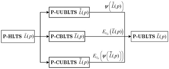
Figure 1.
Transformation relationships between various probabilistic linguistic term sets.
In summary, our newly-defined probabilistic hybrid linguistic term set (P-HLTS) basically contains three new forms of probabilistic linguistic term sets, i.e., P-UUBLTS, P-CBLTS, and P-CUBLTS, which can be transformed into the same form of P-UBLTS [51]. Furthermore, we define the normalized version of P-HLTS in Definition 4.
Definition 5.
Given a P-HLTSwithor, then the associated normalizedis defined as follows:
wherefor all.
Since our newly defined P-HLTS can be transformed and unified into P-UBLTS [51], in the following section, we firstly detail the operational and comparison rules for P-UBLTS, then we propose novel distance and entropy measures for P-UBLTS in Section 3.3.
3.2. Basic Operational Rules and Comparison Rules for P-UBLTS
Definition 6.
[51] Let,, andbe three definite balanced linguistic term sets (BLTSs), and,, andbe three P-HLTS numbers:
,
,
,
Then, by use of equivalent transformation functions [44,62]:
and
, we have
(1)
;
(2);
(3);
(4).
Pang et al. [11] defined the score and deviation degree for probabilistic balanced linguistic term sets (P-BLTSs). Lin et al. [51] extended these definitions and comparison rules into the environment of P-UBLTS, as shown in Definitions 6 and 7.
Definition 7.
[51] If we letbe a P-UBLTS number andbe the subscript of P-UBLTS, then the score ofis given as follows:
The deviation degree ofis given as follows:
Definition 8.
[51] Considering two P-UBLTS numbers ofand, then:
- (1)
- If, then.
- (2)
- If, then.
- (3)
- If, then
- 1)
- If, then.
- 2)
- If, then.
- 3)
- If, then.
3.3. Proposed Distance Measure and Entropy Measure for P-UBLTS
When calculating the distance between any two P-UBLTS numbers, traditional distance measures [63] need to artificially complement, pessimistically or optimistically, certain numbers of elements to the unmatched P-UBLTS number. Either pessimistic complementing or optimistic complementing inevitably brings about information distortion to some extent. Therefore, in the following, we define another distance measure for P-UBLTS numbers without requiring any complementing operation.
Definition 9.
Letandbe two P-UBLTS numbers,andbe the subscripts of P-UBLTSsand, respectively, andandbe the corresponding subscripts of transformed probabilistic uncertain balanced linguistic elementsand, respectively. Here,,. Then, based on the normalized Hamming distance, we define a distance measure as follows:
Situation 1.
When , then:
Situation 2.
When , then:
Theorem 1.
The distance measurefor P-UBLTSs satisfies the following properties:
- (1)
- ;
- (2)
- if;
- (3)
- .
The entropy of fuzzy sets, first mentioned by Zadeh [64] and later widely employed in aggregation operator theories [40,52], is a useful tool to measure the fuzziness of information. Inspired by the entropy measures developed by Liu et al. [40] for probabilistic linguistic term sets (PLTS), we introduce a novel entropy measure for P-UBLTS here.
Definition 10.
Letbe any P-UBLTS element, and, where we then define an entropy measurefor:
Theorem 2.
The entropy defined in the Definition 10 satisfies the following requirements:
- (1)
- ;
- (2)
- , if and only ifor;
- (3)
- , if;
- (4)
- , where;
- (5)
- , ifis less fuzzy than.
4. Prioritized Aggregation Operators for P-UBLTS
Considering that elementary WA and OWA operators cannot accommodate MADM problems with prioritized relationships among evaluative attributes, Yager [52,53] developed another two operators, namely, the fundamental prioritized average (PA) operator [52] and the prioritized ordered weighted aggregation (POWA) operator. Conventional PA and POWA operators generally assume that prioritization relationships among attributes can be determined by DMs or DMUs. When confronting ill-structured, complicated decision situations, the required attributes’ prioritization relationships usually are explicitly unknown and can be objectively derived as order-inducing variables based on acquired decision information [65,66,67,68,69]. Therefore, to facilitate MADM under P-HLTS environments, where decision hesitancy and prioritization relationships between attributes exist, we present the probabilistic uncertain balanced linguistic prioritized weighted average (PUBL-PWA) operator. Furthermore, based on the conventional prioritized aggregation operator [52,53] and induced aggregation operator [65,66], we also develop a probabilistic uncertain balanced linguistic induced prioritized ordered weighted average (PUBL-IPOWA). Desirable properties of the PUBL-PWA and PUBL-IPOWA are also investigated here.
4.1. PUBL-PWA Operator
Definition 11.
where,, andis the entropy ofas calculated according to Definition 11.
Given a collection of P-UBLTS numberswhich are prioritized such thatand,denotes theth uncertain balanced linguistic term and its probability respectively. The PUBL-PWA operator can be defined as follows:
Based on the operations of P-UBLTSs, the PUBL-PWA operator can be rewritten as in Theorem 3.
Theorem 3.
If we letbe a collection of P-UBLTEs, we have
Proof.
(1) When , obviously, it is right.
.
(2) When ,
,
,
,
Thus, Theorem 3 also is right when .
(3) Suppose , then Theorem 3 is right, and we have the following:
.
Then, when ,
.
So, when , Theorem 3 is also correct.
According to steps (1), (2) and (3), we conclude that Theorem 3 is right for all values of . □
Theorem 4.
The PUBL-PWA operator holds the following properties:
(1) Commutativity: Ifis any permutation of, then:
(2) Boundedness: The PUBL-PWA operator lies between the max and min operators:
Proof.
- (1)
- Assume that is any permutation of , then for each , there exists one and only one and vice versa. Additionally, . Thus, based on Theorem 3, we have the following:
- (2)
- Suppose , , then we have the following:
The proof is obvious, thus, details are omitted here. □
Theorem 5.
If any prioritization relationship does not exist, then the PUBL-PWA operator reduces to the PUBL-WA [51] operator:
whereis associated with.
4.2. PUBL-IPOWA Operator
Definition 12.
Given a collection of P-UBLTS numberswhich are prioritized such thatand,denotes theth uncertain balanced linguistic term and its probability, respectively, then the PUBL-IPOWA operator is defined as follows:
whereis a permutation function to generate. Here,is conducted according to an order-inducing vector,, that indicates., whereis the entropy of. Here,,.is a basic unit interval monotonic (BUM) function which satisfies,andif.
Based on the operations of P-UBLTSs, the PUBL-IPOWA operator can be rewritten as in Theorem 6.
Theorem 6.
where
If we letbe a collection of P-UBLTS numbers, andis the reordered collection of, then we have the following:
Proof.
Similar to the proof of Theorem 4, Theorem 6 also can be proved by the mathematical induction method, thus, detailed proof steps are omitted here. □
Theorem 7.
Given a collection of P-UBLTS numbersand the reordered collection ofby a certain order-inducing vector,, iffor all, then the PUBL-IPOWA operator reduces to the PUBL-PWA operator.
Additionally, in resemblance to the proof of Theorem 5, the PUBL-IPOWA operator also holds the properties of commutativity and boundedness.
5. Approaches for MAGDM under Probabilistic Hybrid Linguistic Environments with Decision Hesitancy and Attribute Prioritization Relationships
Aiming to address practical, complicated multiple attribute decision-making problems where decision hesitancy and prioritization relationships exist among the evaluated attributes, in this section, we employ the aforementioned expression tool of P-HLTS and its prioritized aggregation operators to develop two effective MAGDM approaches.
Here, we let be a set of alternatives, be a set of evaluative attributes. Here, represents a set of decision makers (DMs) or decision-making units (DMUs), is the weighting vector for DMs or DMUs, if necessary, , and . Suppose that is the individual decision matrix that contains the preferences given by the th DM or DMU in the form of the probabilistic hybrid linguistic term set (P-HLTS) (i.e., P-UUBLTS, P-CBLTS, or P-CUBLTS) regarding alternative , under the attribute , where and .
Focusing on a specific scenario in which attribute prioritization relationships can be determined in advance and the relative importance of DMs or DMUs are not considered, we firstly construct the following approach.
Approach I.
MAGDM under P-HLTS environments with given prioritization relationships among the evaluated attributes
Suppose that DMs or DMUs have already reached a prioritization relationships among attributes, where indicates that attribute has a higher priority level than .
Step I-1. Transform each individual probabilistic hybrid linguistic decision matrix to in the form of probabilistic uncertain balanced linguistic term sets, then, reorganize according to the prioritization relation .
Step I-2. Construct a synthesized group decision matrix based on individual decision matrices , where . All uncertain balanced linguistic terms are integrated into the uncertain balanced linguistic term set .
Step I-3. Calculate the prioritized weights associated with the PUBL-PWA operator according to the following:
Step I-4. Obtain the aggregate results of each alternative by applying the PUBL-PWA operator:
Step I -5. Calculate and according to Equations (14) and (17).
Step I-6. Based on the rules described in Definition 8, rank all the alternatives and select the most desirable one(s).
Next, regarding decision situations where the relative importance of DMs or DMUs is required but cannot be obtained according to the extant knowledge, or a prioritization relationship does exist among attributes yet cannot be determined based on the extant knowledge of DMs or DMUs, we constructed another approach. During processing in in the second approach, by use of the proposed distance measure for P-HLTS in Definition 9 we develop a method, as shown in Equation (30), that is based on similarity degrees [9] between decision matrices to derive the unknown weight vectors for DMs or DMUs. In essence, the similarity degree-based method allocates higher relative importance to the decision maker or decision-making unit whose decision matrix holds a shorter overall distance from others. To objectively determine the unknown group opinion on prioritization relationships among evaluative attributes, we introduce a divergence measure-based method, as shown in Equations (31) and (32) The divergence measure-based method is grounded in the fact that an attribute under which alternative assessments hold higher divergence is more effective in distinguishing alternatives than certain attributes that provide similar assessments for all alternatives. Therefore, in accordance with the descending order of all divergence measures, we can derive the prioritization relationships among the attributes. The proposed approach is detailed as follows:
Approach II.
MAGDM under P-HLTS environments with unknown attribute prioritization relationships and unknown weights for DMs or DMUs
Step II-1. Transform each individual probabilistic hybrid linguistic decision matrix to in the form of probabilistic uncertain balanced linguistic term sets.
Step II-2. Aggregate all individual decision matrix into the group decision matrix by use of the PUBL-WA operator according to :
where denotes the unknown weights for DMs or DMUs. From the viewpoint of similarity degrees (SDs) between individual decision matrices [9], can be objectively derived according to the following:
Step II-3. Derive the order inducing vector according to descending order of divergence measures of the assessments under each attribute, where we denote the divergence measure by :
Then, according to the order inducing vector , we transform the group decision matrix to the reordered group decision matrix .
Step II-4. Calculate prioritized levels in the group decision matrix , such that the following is true:
Step II-5. Calculate the prioritized weights associated with the PUBL-IPOWA operator, where the following is true:
Step II-6. Obtain the overall group aggregation results of each alternative in the group matrix by applying the PUBL-IPOWA operator, where the following is true:
Step II-7. See Step I-5.
Step II-8. See Step I-6.
For more clarity, Figure 2 shows flowcharts of the proposed approaches.
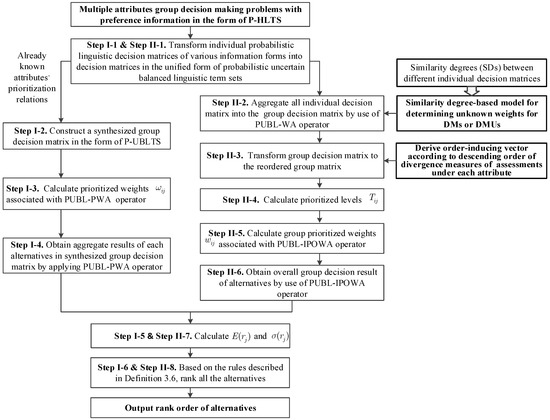
Figure 2.
Flowcharts of Approach I and Approach II.
6. Illustrative Application Study
6.1. Case Study on Governmental Website Usability Evaluation
Along with increasing complexity in their socioeconomic environments, the functionalities of modern governments have diversified to a great extent, especially in developing countries, which are full of socioeconomic dynamics. In order to deliver quality services to stakeholders and increase organizational effectiveness and efficiency, governments at all levels in different areas are trying to establish e-government strategies with the power of information and communication technologies [70]. For example, to guide urbanization rationally and effectively, the Chinese government has put forward national strategies to advocate characteristic towns that combine the functionalities of characteristic industry clusters, cities, communities, and culture and tourism. According to the strategic urbanization system, authorities at the provincial level have been organized and assigned with responsibilities to monitor and guide the development of local characteristic towns. Naturally, fostering and advancing the development of e-governments becomes an imperative part of management tasks for these provincial authorities. According to Baker [71], Clemmensen, and Katre [72], the existing literature has widely argued that e-government efforts will be stifled if e-government websites are not optimally designed to have good usability. Therefore, governments at different levels, such as the aforementioned Chinese provincial authorities, should adopt appropriate decision-making approaches to provide benchmark websites and share excellent experiences among their supervised institutions, so as to continuously improve overall excellence levels in building e-governments. Basically, six attributes of accessibility, information architecture, legitimacy, navigation, online services, and user-help and feedback are commonly utilized to comprehensively evaluate the usability of websites [71]. Essentially, a group of stakeholders should be involved during the process of evaluation, because a single decision maker generally cannot comprehensively consider these six attributes. As seen, MAGDM approaches exhibit intrinsic suitability in solving the complicated problems of comprehensive website usability evaluation.
Suppose that the administrative department in one of Chinese provincial authorities is rallying three decision-making units, namely, users, website developers, and academia experts, in order to determine the benchmarking alternative(s) from four websites . The widely-used six attributes, , for evaluating website usability are adopted here, including accessibility (), information architecture (), legitimacy (), navigation (), online services (), and user-help and feedback (). Here, we let represent the three decision-making units and denote the weighting vectors for the three units if required, and and .
Due to the complexity in comprehensive evaluation and heterogeneity in cognitive models, we use the decision-making units, , to decide whether or not to use P-CUBLTS, P-CBLTS and P-UUBLTS, respectively, for expressing their assessments on the four websites . Here, we use to denote three individual decision matrices. The linguistic variables of in the form of P-CBLTSs have been chosen from the balanced linguistic term set with 16 granularities, and the linguistic variables of in the form of P-UUBLTSs are from the unbalanced linguistic term set, , and the linguistic variables of in the form of P-CUBLTS have been selected from the unbalanced linguistic term set . For more clarity, we demonstrate the relationship between the unbalanced linguistic term sets and in Figure 3. Assessments of the three decision units have been collected in Table 1, Table 2 and Table 3.
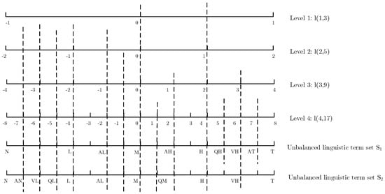
Figure 3.
The relationship between unbalanced linguistic term sets and linguistic hierarchies.

Table 1.
Decision matrix in the form of the probabilistic comparative unbalanced linguistic term set (P-CUBLTS).
Table 2.
Decision matrix in the form of a probabilistic comparative balanced linguistic term set (P-CBLTS).
Table 3.
Decision matrix in the form of probabilistic uncertain unbalanced linguistic term set (P-UUBLTS).
Case I: Suppose that all three decision-making units have reached a consensus on the prioritization relationships among the evaluative attributes, that is , we here firstly apply the first proposed approach to determine the most desirable alternative website(s). The steps for this are organized as follows:
Step I-1. Transform individual decision matrix in the form of P-CUBLTS, in the form of P-CBLTS, and in the form of P-UUBLTS into three decision matrices of , and in the form of probabilistic uncertain balanced linguistic term sets, as shown in Table 4, Table 5 and Table 6.
Table 4.
Transformed decision matrix .
Table 5.
Transformed decision matrix .
Table 6.
Transformed decision matrix .
Step I-2. Based on the three individual decision matrices of , and , we then construct a synthesized group decision matrix , as shown in Table 7.
Table 7.
Group synthesized decision matrix .
Step I-3. Calculate the prioritized weights using Equation (27), where we get the following:
= (0.88653, 0.1019, 0.01012, 0.00134, 0.0001, 0.00001),
= (0.8581, 0.118, 0.02041, 0.0028, 0.00064, 0.00007),
= (0.76016, 0.21138, 0.02298, 0.00467, 0.000716, 0.00009),
= (0.8814, 0.103013, 0.014066, 0.001217, 0.000267, 0.00004).
Step I-4. Obtain the overall group aggregation results of each alternative by Equation (28). For brevity, the details of are omitted here.
Step I-5. Calculate according to Equations (14)–(16), where we have the following:
= 0.7311, = 0.7109, = 0.9005, = 0.8141.
Step I-6. Rank the alternatives according to descending order of , where we then have the following:
Therefore, the best alternative website should be .
Case II: Suppose that the decision-making units have reached a consensus that there is a prioritization relationship among the evaluative attributes, but they cannot explicitly determine the prioritization relationships. In this case, the administrative department advocates that the relative importance of the decision-making units should be differentiated objectively according to their given assessments. Then, we may apply the second approach to solve the above complicated decision-making problem.
Step II-1. See Step I-1.
Step II-2. Determine the weighting vector for the three decision-making units according to Equation (30): . Then, based on the PHUBL-WA operator and the individual matrices in the form of probabilistic uncertain balanced linguistic term sets, we obtain the group decision matrix , as shown in Table 8.
Table 8.
Group decision matrix
Step II-3. By calculating the divergence measure according to Equations (31) and (32), we derive an order-inducing vector in accordance with the descending order of , as listed in Table 9. Then, we can transform to the reordered group decision matrix , according to the order-inducing vector .
Table 9.
Distance values and the corresponding order-inducing vector.
Step II-4. Calculate prioritized levels by Equations (33) and (34), where:
= 1, = 0.028266, = 0.007106, = 0.001869, = 0.000075, = 0.000008;
=1, = 0.30012, = 0.04241, = 0.00499, = 0.00062, = 0.00004;
= 1, = 0.07536, = 0.01369, = 0.00106, = 0.00034, = 0.00004;
= 1, = 0.37335, = 0.032697, = 0.00743, = 0.00041, = 0.000097;
Step II-5. Suppose , then, according to Equation (35), we obtain the attributes’ weighting vectors as follows:
= (0.96402, 0.02725, 0.00685, 0.0018, 0.000072, 0.000008),
= (0.74174, 0.22261, 0.03146, 0.0037, 0.00046, 0.00003),
= (0.91701, 0.06911, 0.01256, 0.00098, 0.00031, 0.00003),
= (0.70722, 0.26404, 0.02312, 0.00526, 0.00029, 0.00007).
Step II-6. Obtain overall group aggregation results by Equation (36). Please note that details about are omitted here for brevity.
Step II-7. Calculate according to Equations (14)–(16), and we have:
= 0.7415, = 0.8525, = 0.839, = 0.8073.
Step II-8. Rank the alternatives according to descending order of :
Therefore, the best alternative is .
6.2. Comparative Studies
6.2.1. Comparative Experiments with Various Configurations of and
To further verify our approaches, in this section, we conduct more experiments on the two approaches with different configurations of the weighting vector, , for the DMUs and the attributes’ prioritization relationships, . The experimental data and the obtained ranking results are presented in Table 10.
Table 10.
Comparative experiments on the proposed approaches with various configurations of and .
According to experiments I-1 and II-1, where both approaches I and II did not emphasize the relative importance of DMUs and the relative importance of the evaluative attributes, approaches I and II both identified as the best website and as the worst website. The ranking results show that both approaches are effective for tackling complicated problems that require assessments in the form of P-HLTS and hold no specific information on and .
In experiments I-2 and I-3, approach I used with two configurations of : (i) , given directly by DMUs based on their consensus opinion, and (ii) , derived by the divergence measure-based method in Equations (31) and (32). Ranking results in Table 10 showed the same permutation of the four alternative websites. In comparison with the result from experiment I-1 with approach I, the alternative value became the worst alternative in response to the attributes’ prioritization relationships. Regarding the experiments for approach II in which the weight vectors of DMUs were explicitly incorporated, different from II-1, experiments II-2 and II-3 both proceeded with the attributes’ prioritization relationships, i.e., , which was derived by the divergence measure-based method. Under the influence of the attributes’ prioritization relations , the alternative was recognized as the best website. As shown in Table 10, because , derived in experiment II-3, has tiny differences from , adopted in experiment II-2, experiment II-3 outputs the same ranking order as in experiment II-2. As can be seen from the above observation and analysis, decision makers’ opinions on attributes’ prioritization relationships substantially influences the decision results. Both approaches manage to accommodate the important opinions in their decision-making processes and reflect influences in ranking results accordingly. Generally, our proposed approaches present effective methodologies for MAGDM problems in P-HLTS environments where weighting vectors for DMs or DMUs and attribute prioritization relationships are known or explicitly unknown.
6.2.2. Comparative Experiments with Different Approaches
Consequently, because the various expression forms included in our proposed probabilistic hybrid linguistic term set (P-HLTS) can be transformed into the form of a probabilistic uncertain linguistic set [51] and both references [51], and since our research has been conducted to study MADM in group decision-making settings, we used the original synthesized group decision-making matrix in [51] for comparative experiments. The weight for decision makers is thus not considered. Then, we configured our first proposed approach as shown in the experiment I-3 in Table 10, that is, we objectively calculate the order-inducing vector based on the synthesized group decision matrix adopted in [51], then compare the corresponding ranking results as collected in Table 11.
Table 11.
Comparative experiments with different approaches.
In light of the comparative method in [51], which was constructed based on classic TOPSIS method, we here denote their method as extended TOPSIS in Table 11. Please note that our adapted first approach takes the synthesized group decision matrix, thereby using objectively derived to guide the decision-making process, thus, the adapted first approach can be seen as a special case of our second proposed approach. Furthermore, to further verify the ranking results of our approach, we also constructed another approach to solve the same problem, named prioritized TOPSIS in Table 11, by integrating the TOPSIS framework and the -guided attribute weights.
As seen from Table 11, after introducing the -guided priority relationships among the evaluative attributes, both the adapted approach I and prioritized TOPSIS approach output different ranking results from the results generated by the extended TOPSIS [51]. Both the extended TOPSIS and the prioritized TOPSIS approaches inherit the robust decision-making process of the classic TOPSIS method, but the difference lies in that the prioritized TOPSIS approach integrates -guided priority relationships among attributes and generates the ranking result of . Additionally, as can be seen via comparison of the result obtained by our proposed approach, both adapted approach I and prioritized TOPSIS indicate the best alternative as and the worst alternative as . Therefore, generally speaking, for situations where attributes’ prioritization relationships are explicitly unknown, our proposed approaches provide a way of objectively determining -guided priority relationships and effectively integrate priority relationships in MAGDM under P-HLTS environments in order to derive rational decision results.
6.3. Sensitivity Analysis
When tackling complicated multiple attribute decision-making problems where prioritization relationships exist among evaluative attributes, Yager [52] and Yager [53] have presented effective ways of deriving decision-making results by utilizing prioritized aggregation operators. During information aggregation, priority relationships among attributes and scope relationships among attributes generally should be taken into consideration [52,53]. Normalized priority importance weights for attributes can be calculated according to specified priority relationships. For decision-making scenarios of high complexity, where no concrete vectors exist for describing the scope of relationships among attributes, Yager [52,53,73] suggested employing as basic, unit interval, and monotonic (BUM) functions to express the implicit scope relationships among the attributes. To the best of our knowledge, in the literature, [52,53,58,73,74] and [52,53,73,74] have been usually suggested for multiple attribute decision-making. Therefore, in this subsection, to examine the effects of various BUM functions on the decision results of our proposed approaches, we have carried out sensitivity analysis through the use of the functions and the results are presented in Table 12.
Table 12.
Ranking results by approaches I and II with various basic, unit interval, and monotonic (BUM) functions.
As shown in Table 12, we have carried out experiments on approach I (on the group synthesized decision matrix in Table 7) and approach II (on the aggregated group decision matrix in Table 8) to examine effects of five BUM functions on ranking results, respectively. Regarding the experiments on approach I, ranking results by all five functions indicate that the alternative is the best one. Here, , and all obtain exactly the same ranking result, while the other two functions yield different permutations of and . In regard to experiments on approach II, , , , and all obtain exactly the same ranking result, while yields different permutations of and . As can be observed, and exhibit consistent ranking results in the above experiments, which is in accordance with the suggestions in the literature. Therefore, when applying our proposed approaches to complicated decision-making scenarios where prioritization relationships exist among evaluative attributes but no concrete descriptions of scope relationships among attributes exist, or is suggested. In addition, it is worth mentioning that more precise BUM functions should be constructed if specific vectors exist for describing scope relationships among attributes, such as the piecewise linear functions suggested by Torra [75] and Torra and Narukawa [76].
6.4. Further Discussion: Vector Optimization Based Approach to Solving Website Usability Evaluation with Priority Attributes
During the preceding parts, we have developed and verified two MAGDM approaches based on DM assessments of comprehensively evaluated website usability in accordance with governmental design requirements, which is usually arranged as a typical task of government departments in China.
However, from the systemic view [77] of the operational management of websites, technical observations and empirical studies generally can identify a set of technical parameters, , that are closely associated with the system characteristics regarding website usability (denoted as the aforementioned six attributes ). Due to complexity and uncertainty in practical scenarios, the values of some parts of parameters and attributes usually have to be expressed in uncertain forms, including linguistic variables and probabilistic hybrid linguistic term sets, etc. Especially, similar to the description in the preceding case study, priority relationships also will exist among the attributes as guided by specific operational management arrangements. Additionally, the task of this type of website usability evaluation presents problems regarding the priority attributes which are used to make the best decision (optimal ) with the collected data and given guiding priority relationships among attributes.
More specifically, a technical system’s (e-governmental website) usability function is defined by the vector of parameters . Operation of the technical system is determined by six characteristics (six attributes in the above case), the values of which are recognized as being associated with the vector of parameters : . The values of the parameters and characteristics of the technical system are shown in Table 13.
Table 13.
Collected values of the parameters and characteristics of the technical system.
In the light of Mashunin and Mashunin [78], the above website usability evaluation problem can be constructed and successfully solved as a type of vector problem of mathematical programming, and its solution steps can be explained in a general form as in the following approach.
Approach III.
Vector optimization-based [78] decision-making steps in a general form for website usability evaluation
Step III-1. Collect initial data of parameters and six characteristics . If these were originally obtained in various forms of uncertain expressions, utilize appropriate transformative methods (such as the mapping function [30] for linguistic scales or the score function [51] for P-HLTS) to get the numerical values of these parameters and characteristics, as organized in Table 13. Determine constraints for both parameters and possible functional attributes. In the decision taken, it is desirable to obtain the values of all characteristics such that they are as high as possible (i.e., at a maximum).
Step III-2. Utilize regression analysis methods, such that the discrete data sets of , , , , , and are respectively converted into six functions of , , , , , and . These six functions are then used as attributes in the vector problem of mathematical programming [78]: , , , , , and .
Step III-3. Solve the above vector problem of mathematical programming with equivalent attributes [79].
Step III-4. According to specific operational management arrangements, decision makers decide to choose priority attributes and determine the numerical value of the corresponding priority attributes.
Step III-5. With the given attribute priority, Mashunin and Mashunin’s [78] methods are used to obtain the optimal parameter vector within the assigned error range.
As pointed by Mashunin and Mashunin [78], the above approach of optimal decision-making with an assigned attribute priority is based on the axioms with the use of the normalization of attributes and the max-min principle, and the accuracy of choosing such an optimal parameter vector depends on a predetermined error range. Regarding the specific implementation of the vector optimization methods, of which the third approach presented here depends on, one can refer to references [78,79] for great insight in this regard. After the acceptable optimal vector is obtained and the optimal parameters are further analyzed according to concrete scenarios, managerial suggestions for operational improvements thus can be deduced more reasonably.
7. Conclusions
Aiming to deal with ill-structured, complicated problems under linguistic MADM scenarios, we have introduced a more comprehensive expression tool for P-HLTSs to depict decision hesitancy concerning possible linguistic labels and the probabilistic preferences on those linguistic labels. P-HLTSs enhance classical probabilistic linguistic term sets through encompassing a wide range of linguistic expression forms when answering diverse cognitive models, including balanced linguistic sets, unbalanced linguistic term sets, uncertain unbalanced linguistic term sets, comparative balanced linguistic term sets, and comparative unbalanced linguistic term set. For MADM under complicated situations, where decision makers cannot determine concrete weighting vectors for attributes but have opinions on attributes’ prioritization relationships, we have developed two important information aggregation operators (PUBL-PWA and PUBL-IPOWA), used to accommodate the specific decision opinions. Then, based on the above tools, with respect to practical MADM problems where weighting vector for DMs or DMUs and attributes’ prioritization relationships are known or explicitly unknown, we have constructed two effective MAGDM approaches, respectively. Additionally, through application study and comparative experiments we have validated the two approaches.
Since the newly-introduced expression tool of P-HLTS behaves more flexibly and comprehensively when eliciting probabilistic linguistic decision information, future research efforts should be directed to studying effective aggregation operators for various practical contexts, thereby developing appropriate MADM methodologies for real applications. Another promising research direction should be well-explored and exploited by integrating MADM methodologies and vector optimization theories.
Author Contributions
Conceptualization, C.L.; Formal analysis, X.Q.; Funding acquisition, J.Z.; Investigation, X.Q.; Methodology, X.Q.; Resources, Y.H. and C.L.; Supervision, J.Z.; Validation, Y.H.; Writing–original draft, J.Z. All authors have read and agreed to the published version of the manuscript.
Funding
This paper was fully supported by The National Social Science Fund of China, grant number 17BJY159.
Conflicts of Interest
The authors declare that there is no conflict of interest regarding the publication of this paper.
Appendix A
Definition A1.
[27] Given a certain linguistic hierarchy, in which all included linguistic term sets are denoted as, for the purpose of transforming from a linguistic label in levelto a label in consecutive level, a transformation function is defined as: such that the following is true:
Utilizing the function , any 2-tuple linguistic expression can be transformed into a term in . More specifically, transformation procedures by use of are detailed as follows:
(1) Mapping process: To map an unbalanced term set to its corresponding terms in , a transformation function is determined to relate to every unbalanced linguistic 2-tuple to its linguistic 2-tuple in , i.e.:
where we then we have for .
(2) Computing process: Here, we transform into linguistic 2-tuples which are denoted as :
We then apply the computational model to and the corresponding result is denoted as .
(3) Retranslating process: Next, is transformed into an unbalanced term in through the transformation function , i.e.:
where we then we get .
References
- Zimmerman, H.J. Fuzzy Set Theory and Its Applications; Springer: Dordrecht, The Netherlands, 2001. [Google Scholar]
- Liu, P.D.; Wu, X.Y. A competency evaluation method of human resources managers based on multi-granularity linguistic variables and vikor method. Technol. Econ. Dev. Econ. 2012, 18, 696–710. [Google Scholar] [CrossRef]
- Liu, P. Multiple attribute group decision making method based on interval-valued intuitionistic fuzzy power heronian aggregation operators. Comput. Ind. Eng. 2017, 108, 199–212. [Google Scholar] [CrossRef]
- Liu, P. A weighted aggregation operators multi-attribute group decision-making method based on interval-valued trapezoidal fuzzy numbers. Appl. Math. Model. 2011, 38, 1053–1060. [Google Scholar] [CrossRef]
- Ju, Y.; Yang, S. Approaches for multi-attribute group decision making based on intuitionistic trapezoid fuzzy linguistic power aggregation operators. J. Intell. Fuzzy Syst. 2014, 27, 987–1000. [Google Scholar] [CrossRef]
- Ju, Y.; Yang, S. A new method for multiple attribute group decision-making with intuitionistic trapezoid fuzzy linguistic information. Soft Comput. 2015, 19, 2211–2224. [Google Scholar] [CrossRef]
- Ju, Y.; Yang, S.; Liu, X. A novel method for multiattribute decision making with dual hesitant fuzzy triangular linguistic information. J. Appl. Math. 2014, 2014, 12. [Google Scholar] [CrossRef]
- Wu, J.; Chang, J.; Cao, Q.; Liang, C. A trust propagation and collaborative filtering based method for incomplete information in social network group decision making with type-2 linguistic trust. Comput. Ind. Eng. 2019, 127, 853–864. [Google Scholar] [CrossRef]
- Qi, X.; Liang, C.; Zhang, J. Generalized cross-entropy based group decision making with unknown expert and attribute weights under interval-valued intuitionistic fuzzy environment. Comput. Ind. Eng. 2015, 79, 52–64. [Google Scholar] [CrossRef]
- Qi, X.; Liang, C.; Zhang, J. Multiple attribute group decision making based on generalized power aggregation operators under interval-valued dual hesitant fuzzy linguistic environment. Int. J. Mach. Learn. Cybern. 2016, 7, 1147–1193. [Google Scholar] [CrossRef]
- Pang, Q.; Wang, H.; Xu, Z. Probabilistic linguistic term sets in multi-attribute group decision making. Inf. Sci. 2016, 369, 128–143. [Google Scholar] [CrossRef]
- Zhao, S.; Wang, D.; Liang, C.; Leng, Y.; Xu, J. Some single-valued neutrosophic power heronian aggregation operators and their application to multiple-attribute group decision-making. Symmetry 2019, 11, 653. [Google Scholar] [CrossRef]
- Zhang, J.; Qi, X.; Liang, C. Tackling complexity in green contractor selection for mega infrastructure projects: A hesitant fuzzy linguistic madm approach with considering group attitudinal character and attributes’ interdependency. Complexity 2018, 2018, 31. [Google Scholar] [CrossRef]
- Wei, G.; Zhao, X. Some induced correlated aggregating operators with intuitionistic fuzzy information and their application to multiple attribute group decision making. Expert Syst. Appl. 2012, 39, 2026–2034. [Google Scholar] [CrossRef]
- Wei, G. Interval valued hesitant fuzzy uncertain linguistic aggregation operators in multiple attribute decision making. Int. J. Mach. Learn. Cybern. 2016, 7, 1093–1114. [Google Scholar] [CrossRef]
- Ju, Y.B. A new method for multiple criteria group decision making with incomplete weight information under linguistic environment. Appl. Math. Model. 2014, 38, 5256–5268. [Google Scholar] [CrossRef]
- Ju, Y.B.; Wang, A.H.; You, T.H. Emergency alternative evaluation and selection based on anp, dematel, and tl-topsis. Nat. Hazards 2015, 75, S347–S379. [Google Scholar] [CrossRef]
- Zadeh, L.A. Fuzzy sets. Inf. Control 1965, 8, 338–353. [Google Scholar] [CrossRef]
- Atanassov, K.T. Intuitionistic fuzzy sets. Fuzzy Sets Syst. 1986, 20, 87–96. [Google Scholar] [CrossRef]
- Atanassov, K.T.; Gargov, G. Interval valued intuitionistic fuzzy sets. Fuzzy Sets Syst. 1989, 31, 343–349. [Google Scholar] [CrossRef]
- Torra, V. Hesitant fuzzy sets. Int. J. Intell. Syst. 2010, 25, 529–539. [Google Scholar] [CrossRef]
- Zhu, B.; Xu, Z.S.; Xia, M.M. Dual hesitant fuzzy sets. J. Appl. Math. 2012, 2012, 13. [Google Scholar] [CrossRef]
- Ju, Y.B.; Liu, X.Y.; Yang, S.H. Interval-Valued dual hesitant fuzzy aggregation operators and their applications to multiple attribute decision making. J. Intell. Fuzzy Syst. 2014, 27, 1203–1218. [Google Scholar] [CrossRef]
- Hao, Z.; Xu, Z.; Zhao, H.; Su, Z. Probabilistic dual hesitant fuzzy set and its application in risk evaluation. Knowl. Based Syst. 2017, 127, 16–28. [Google Scholar] [CrossRef]
- Zadeh, L.A. The concept of a linguistic variable and its application to approximate reasoning-i. Inf. Sci. 1975, 8, 199–249. [Google Scholar] [CrossRef]
- Herrera-Viedma, E.; López-Herrera, A.G. A model of an information retrieval system with unbalanced fuzzy linguistic information. Int. J. Intell. Syst. 2007, 22, 1197–1214. [Google Scholar] [CrossRef]
- Herrera, F.; Herrera-Viedma, E.; Martinez, L. A fuzzy linguistic methodology to deal with unbalanced linguistic term sets. IEEE Trans. Fuzzy Syst. 2008, 16, 354–370. [Google Scholar] [CrossRef]
- Martínez, L.; Espinilla, M.; Liu, J.; Pérez, L.G.; Sánchez, P.J. An evaluation model with unbalanced linguistic information applied to olive oil sensory evaluation. J. Mult. Valued Log. Soft Comput. 2009, 15, 229–251. [Google Scholar]
- Cai, M.; Gong, Z.; Yu, X. A method for unbalanced linguistic term sets and its application in group decision making. Int. J. Fuzzy Syst. 2016, 19, 1–12. [Google Scholar] [CrossRef]
- Xu, Z.S. Uncertain linguistic aggregation operators based approach to multiple attribute group decision making under uncertain linguistic environment. Inf. Sci. 2004, 168, 171–184. [Google Scholar] [CrossRef]
- Wei, G.; Zhao, X.; Lin, R.; Wang, H. Uncertain linguistic bonferroni mean operators and their application to multiple attribute decision making. Appl. Math. Model. 2013, 37, 5277–5285. [Google Scholar] [CrossRef]
- Liu, P.; Yu, X. 2-Dimension uncertain linguistic power generalized weighted aggregation operator and its application in multiple attribute group decision making. Knowl. Based Syst. 2014, 57, 69–80. [Google Scholar] [CrossRef]
- Liu, P.; He, L.; Yu, X. Generalized hybrid aggregation operators based on the 2-dimension uncertain linguistic information for multiple attribute group decision making. Group Decis. Negot. 2016, 25, 103–126. [Google Scholar] [CrossRef]
- Liu, P. Some geometric aggregation operators based on interval intuitionistic uncertain linguistic variables and their application to group decision making. Appl. Math. Model. 2013, 37, 2430–2444. [Google Scholar] [CrossRef]
- Meng, F.; Chen, X.; Zhang, Q. Some interval-valued intuitionistic uncertain linguistic choquet operators and their application to multi-attribute group decision making. Appl. Math. Model. 2014, 38, 2543–2557. [Google Scholar] [CrossRef]
- Qi, X.-W.; Zhang, J.-L.; Liang, C.-Y. Multiple attributes group decision-making under interval-valued dual hesitant fuzzy unbalanced linguistic environment with prioritized attributes and unknown decision-makers’ weights. Information 2018, 9, 145. [Google Scholar] [CrossRef]
- Rodríguez, R.M.; Martínez, L.; Herrera, F. Hesitant fuzzy linguistic term sets for decision making. IEEE Trans. Fuzzy Syst. 2012, 20, 109–119. [Google Scholar] [CrossRef]
- Liao, H.; Jiang, L.; Xu, Z.; Xu, J.; Herrera, F. A linear programming method for multiple criteria decision making with probabilistic linguistic information. Inf. Sci. 2017, 415, 341–355. [Google Scholar] [CrossRef]
- Xie, W.; Ren, Z.; Xu, Z.; Wang, H. The consensus of probabilistic uncertain linguistic preference relations and the application on the virtual reality industry. Knowl. Based Syst. 2018, 162, 14–28. [Google Scholar] [CrossRef]
- Liu, H.; Le, J.; Xu, Z. Entropy measures of probabilistic linguistic term sets. Int. J. Comput. Intell. Syst. 2018, 11, 45–87. [Google Scholar] [CrossRef]
- Wu, X.; Liao, H. An approach to quality function deployment based on probabilistic linguistic term sets and oreste method for multi-expert multi-criteria decision making. Inf. Fusion 2018, 43, 13–26. [Google Scholar] [CrossRef]
- Xiang, C.; Jing, G.; Xu, Z. Venture capital group decision-making with interaction under probabilistic linguistic environment. Knowl. Based Syst. 2018, 140, 82–91. [Google Scholar]
- Gao, J.; Xu, Z.; Ren, P.; Liao, H. An emergency decision making method based on the multiplicative consistency of probabilistic linguistic preference relations. Int. J. Mach. Learn. Cybern. 2019, 10, 1613–1629. [Google Scholar] [CrossRef]
- Bai, C.Z.; Zhang, R.; Qian, L.X.; Wu, Y.N. Comparisons of probabilistic linguistic term sets for multi-criteria decision making. Knowl. Based Syst. 2017, 119, 284–291. [Google Scholar] [CrossRef]
- Liu, P.; You, X. Probabilistic linguistic todim approach for multiple attribute decision-making. Granul. Comput. 2017, 2, 333–342. [Google Scholar] [CrossRef]
- Zhang, X.; Xing, X. Probabilistic linguistic vikor method to evaluate green supply chain initiatives. Sustainability 2017, 9, 1231. [Google Scholar] [CrossRef]
- Rodríguez, R.M.; Martínez, L.; Herrera, F. A group decision making model dealing with comparative linguistic expressions based on hesitant fuzzy linguistic term sets. Inf. Sci. 2013, 241, 28–42. [Google Scholar] [CrossRef]
- Wang, H. Extended hesitant fuzzy linguistic term sets and their aggregation in group decision making. Int. J. Comput. Intell. Syst. 2015, 8, 14–33. [Google Scholar] [CrossRef]
- Liu, P.; Fei, T. Some muirhead mean operators for probabilistic linguistic term sets and their applications to multiple attribute decision-making. Appl. Soft Comput. 2018, 68. [Google Scholar] [CrossRef]
- Liu, P.; Li, Y. Multi-Attribute decision making method based on generalized maclaurin symmetric mean aggregation operators for probabilistic linguistic information. Comput. Ind. Eng. 2019, 131, 282–294. [Google Scholar] [CrossRef]
- Lin, M.W.; Xu, Z.S.; Zhai, Y.L.; Yao, Z.Q. Multi-Attribute group decision-making under probabilistic uncertain linguistic environment. J. Oper. Res. Soc. 2018, 69, 157–170. [Google Scholar] [CrossRef]
- Yager, R.R. Prioritized aggregation operators. Int. J. Approx. Reason. 2008, 48, 263–274. [Google Scholar] [CrossRef]
- Yager, R.R. Prioritized owa aggregation. Fuzzy Optim. Decis. Mak. 2009, 8, 245–262. [Google Scholar] [CrossRef]
- Yager, R.R. Prioritized aggregation operators and their applications. In Proceedings of the 6th IEEE International Conference Intelligent Systems (IS), Sofia, Bulgaria, 6–8 September 2012; pp. 2–5. [Google Scholar]
- Yu, X.H.; Xu, Z.S. Prioritized intuitionistic fuzzy aggregation operators. Inf. Fusion 2013, 14, 108–116. [Google Scholar] [CrossRef]
- Yu, D.; Wu, Y.; Lu, T. Interval-Valued intuitionistic fuzzy prioritized operators and their application in group decision making. Knowl. Based Syst. 2012, 30, 57–66. [Google Scholar] [CrossRef]
- Wei, G. Hesitant fuzzy prioritized operators and their application to multiple attribute decision making. Knowl. Based Syst. 2012, 31, 176–182. [Google Scholar] [CrossRef]
- Jin, F.; Ni, Z.; Chen, H. Interval-Valued hesitant fuzzy einstein prioritized aggregation operators and their applications to multi-attribute group decision making. Soft Comput. 2016, 20, 1863–1878. [Google Scholar] [CrossRef]
- Zhang, S.; Xu, Z.; He, Y. Operations and integrations of probabilistic hesitant fuzzy information in decision making. Inf. Fusion 2017, 38, 1–11. [Google Scholar] [CrossRef]
- Marin, L.; Merigó, J.M.; Valls, A.; Moreno, A.; Isern, D. Induced unbalanced linguistic ordered weighted average. Sci. World J. 2011, 1, 1–8. [Google Scholar]
- Marin, L.; Valls, A.; Isern, D.; Moreno, A.; Merigó, J.M. Induced unbalanced linguistic ordered weighted average and its application in multiperson decision making. Sci. World J. 2014, 2014, 19. [Google Scholar] [CrossRef]
- Gou, X.; Xu, Z.; Liao, H. Multiple criteria decision making based on bonferroni means with hesitant fuzzy linguistic information. Soft Comput. 2016, 21, 1–15. [Google Scholar] [CrossRef]
- Wei, G.; Lin, R.; Wang, H. Distance and similarity measures for hesitant interval-valued fuzzy sets. J. Intell. Fuzzy Syst. 2014, 27, 19–36. [Google Scholar] [CrossRef]
- Zadeh, L.A. Probability measures of fuzzy events. J. Math. Anal. Appli. 1968, 23, 421–427. [Google Scholar] [CrossRef]
- Yager, R.R.; Filev, D.P. Induced ordered weighted averaging operators. IEEE Trans. Syst. Man Cybern. Part B Cybern. 1999, 29, 141–150. [Google Scholar] [CrossRef] [PubMed]
- Yager, R.R. Induced aggregation operators. Fuzzy Sets Syst. 2003, 137, 59–69. [Google Scholar] [CrossRef]
- Chen, H.; Zhou, L. An approach to group decision making with interval fuzzy preference relations based on induced generalized continuous ordered weighted averaging operator. Expert Syst. Appl. 2011, 38, 13432–13440. [Google Scholar] [CrossRef]
- Merigó, J.M.; Casanovas, M. Induced aggregation operators in the euclidean distance and its application in financial decision making. Expert Syst. Appl. 2011, 38, 7603–7608. [Google Scholar] [CrossRef]
- Zhou, L.G.; Chen, H.Y. The induced linguistic continuous ordered weighted geometric operator and its application to group decision making. Comput. Ind. Eng. 2013, 66, 222–232. [Google Scholar] [CrossRef]
- Verkijika, S.F.; de Wet, L. A usability assessment of e-government websites in Sub-Saharan Africa. Int. J. Inf. Manag. 2018, 39, 20–29. [Google Scholar] [CrossRef]
- Baker, D.L. Advancing e-government performance in the united states through enhanced usability benchmarks. Gov. Inf. Q. 2009, 26, 82–88. [Google Scholar] [CrossRef]
- Clemmensen, T.; Katre, D. Chapter 21—Adapting e-gov usability evaluation to cultural contexts. In Usability in Government Systems; Buie, E., Murray, D., Eds.; Morgan Kaufmann: Boston, MA, USA, 2012; pp. 331–344. [Google Scholar]
- Yager, R.R. On the inclusion of importances in owa aggregations. In The Ordered Weighted Averaging Operators; Yager, R.R., Kacprzyk, J., Eds.; Springer: Boston, MA, USA, 1997. [Google Scholar]
- Li, B.; Xu, Z. Prioritized aggregation operators based on the priority degrees in multicriteria decision-making. Int. J. Intell. Syst. 2019, 34, 1985–2018. [Google Scholar] [CrossRef]
- Torra, V. The weighted owa operator. Int. J. Intell. Syst. 1997, 12, 153–166. [Google Scholar] [CrossRef]
- Torra, V.; Narukawa, Y. Modeling Decisions: Information Fusion and Aggregation Operators; Springer: Berlin, Germany, 2007. [Google Scholar]
- Mashunin, K.Y.; Mashunin, Y.K. Simulating engineering systems under uncertainty and optimal decision making. J. Comput. Syst. Sci. Int. 2013, 52, 519–534. [Google Scholar] [CrossRef]
- Mashunin, K.Y.; Mashunin, Y.K. Vector optimization with equivalent and priority criteria. J. Comput. Syst. Sci. Int. 2017, 56, 975–996. [Google Scholar] [CrossRef]
- Mashunin, Y.K. Methods and Models of Vector Optimization; Nauka: Moscow, Russia, 1986. [Google Scholar]
© 2020 by the authors. Licensee MDPI, Basel, Switzerland. This article is an open access article distributed under the terms and conditions of the Creative Commons Attribution (CC BY) license (http://creativecommons.org/licenses/by/4.0/).