Symmetric Properties of Eigenvalues and Eigenfunctions of Uniform Beams

Abstract

In this paper, the models of Euler–Bernoulli beams on the Winkler foundations are considered. The novelty of the research is in consideration of the models with an arbitrary variable coefficient of foundation. Qualitative results that influence the symmetry of the coefficient of foundation on the spectral properties of the corresponding problems are obtained, for which specific variable coefficients of foundation are tested using numerical calculations. Three types of fixing at the ends are studied: clamped-clamped, hinged-hinged and free-free. The conditions of the stiffness and types of beam fixing have been found for the set of eigenvalues of boundary value problems on a full segment and can be represented as two groups of the eigenvalues of certain problems on a half segment. Such qualitative spectral properties of a mechanical system can contribute to the creation of various algorithms for nondestructive testing, which are widely used in technical acoustics.

1. Introduction

In this paper, the eigenvalues of a uniform Euler–Bernoulli beam lying on a Winkler’s type foundation at three types of fixings at the ends are studied: clamped-clamped, hinged-hinged and free-free [1]. The spectral properties of a mechanical system under any type of oscillations resting on elastic foundations have a wide range of applications in different science and engineering areas. These properties are used for modeling railway tracks, bridges, pavements, runways, pipelines, piles, etc. (see [1,2,3,4]).

Let $k\left(x\right),x\in (0;1)$ be a real-valued summable function, and $\lambda$ is an eigenvalue. A force of foundation reaction is equal:

$$p\left(x\right)=k\left(x\right)w(x,t),$$

where $k\left(x\right)$ is the variable coefficient of foundation $(\mathrm{kN}\hspace{0.17em}{\mathrm{m}}^{-1})$ and $w(x,t)$ is the transverse displacement $\left(\mathrm{m}\right)$. The properties of the eigenvalues and eigenfunctions of boundary value problems for the Euler–Bernoulli beam with a constant coefficient of foundation were studied well. The comprehensive review on different theoretical elastic and viscoelastic foundation models in oscillatory systems can be found in [4]. The foundation of a mechanical system is generally described by a variable coefficient in numerous applied mathematical models. If the foundation coefficient is variable, then the question of studying the qualitative behaviors of the eigenvalues and eigenfunctions arises. Analytical solutions are not always obtained in an explicit form with a variable coefficient, as in the case of a constant coefficient.

Attempts to estimate the coefficients of foundation of a mechanical system were carried out in [5,6,7]. The approximate solutions of free vibrations in the integral form and Taylor series expansion for a uniform beam on a linear variable coefficient of foundation were considered in [2] (p. 109) and [8] (p. 26). Clastornik et al. [9] studied the approximation solution for finite beams with a polynomial coefficient $k\left(x\right)={\sum }_{n=1}^{\infty }{k}_n{x}^n$. The case of the variable coefficient of foundation where it is given as the random stiffness following form $k\left(x\right)=k_0+k_{\epsilon }\left(x\right)$, where $k_0=const,$ $k_{\epsilon }\left(x\right)$ is the longitudinal variations of stiffness, was considered in [10,11,12].

Natural frequencies of the Euler–Bernoulli beam for the linear $k\left(x\right)=k_0(1-\alpha x),\hspace{0.17em}0\le \alpha \le 1$ and the nonlinear $k\left(x\right)=k_0(1-\beta x^2),\hspace{0.17em}0\le \beta \le 1$ functions were investigated in [13,14]. In [13], the general solution of the vibrations of uniform beams on variable Winkler elastic foundations were derived. In [14], the method of differential transformation was applied. In [3], the explicit form of the solution of the fourth order differential equation for $k\left(x\right)=\frac{1}{{\left(c_0+c_{1}x\right)}^4}$ with hinged-hinged of fixing and at constant external load was obtained. In [15], the explicit solution static bending response of a finite uniform free-free Euler–Bernoulli beam resting on a Winkler elastic foundation in terms of special functions was derived. The boundary value problems for ordinary high-order differential operators in which the spectrum is absent or the spectrum is a countable set were considered in the case with constant coefficients in [16] and with variable coefficients in [17]. The odd order differential operators for the similar questions were investigated in [18,19]. The eigenvalues of the two-point boundary value problem of the ordinary differential operator for a triple differentiation with asymmetric weight were studied in [19]. In [20,21], these ones were studied for the second-order differential operators. The class of Volterra three-point problems for the Sturm–Liouville operator on the closed interval were described in [21]. Here, the Volterra was related to the double symmetry of the potential. The research methods used in this work develop the methods of works from [19,21].

It is important to develop the numerical methods together with the qualitative methods to study the spectral properties of the differential operators and allow one to test the correctness of quality results. Recently, based on the numerical methods for estimation of the eigenvalues, the variational iteration methods [22], the Haar wavelet method [23], the differential quadrature method and the Boubaker polynomials expansion scheme [24], the polynomial expansion and the integral technique methods [25], the Chebyshev spectral Method [26] was developed.

Basically, the effective methods for the numerical calculation of the eigenvalues of the fourth-order differential equation with definite variable coefficients were developed in [8,9,10,11,12,13,14,22,23,24,25,26]. However, they did not study the qualitative properties of the eigenvalues. In particular, these works did not consider the influence of the coefficients of the equation to the spectrum factorization. It is difficult to reveal such spectral properties of the system using numerical calculations. Here, it is necessary to use qualitative properties (symmetry).

In science, questions often arise to generalize well-known classical results for clearer understanding of the system properties and more detailed analysis. For instance, the first four alternating symmetric and asymmetric eigenfunctions with respect to the middle of uniform clamped-clamped Euler–Bernoulli beam without an elastic foundation (Winkler’s coefficient is identically equal to zero) were defined in [27] (p. 270). An assumption was formulated that this tendency was preserved for all other eigenfunctions. A research problem arises, then: which nonzero coefficients of the Winkler foundation of this property are preserved? The novelty of this work is defining a condition for a nonzero variable coefficient of foundation under the symmetric properties of the eigenfunctions of the beam are preserved (see Theorem 1). Factorization of the set of eigenvalues was carried out. Similar results for other fixing types of beams were obtained (see Theorems 2 and 3).

The goal of this study is to find conditions for a variable coefficient of foundation and fixing types of a beam under which it is possible to establish the qualitative behavior of the eigenvalues and eigenfunctions. According to the authors’ assumption, an important factor to achieve the goal is the symmetric properties of the variable coefficient of foundation and corresponding fixing types of beam.

The work is organized as follows. After the introduction, a mathematical model of free transverse vibration of the Euler–Bernoulli beam lying on a Winkler’s type foundation are formulated. Eigenvalues and eigenfunctions with three types of fixings at the ends are investigated: clamped-clamped, hinged-hinged and free-free. In the third section, the examples are given to illustrate the results. Finally, main conclusions are outlined in closing.

2. The Problem of Transverse Vibrations of a Beam Lying on a Winkler’s Type Foundation

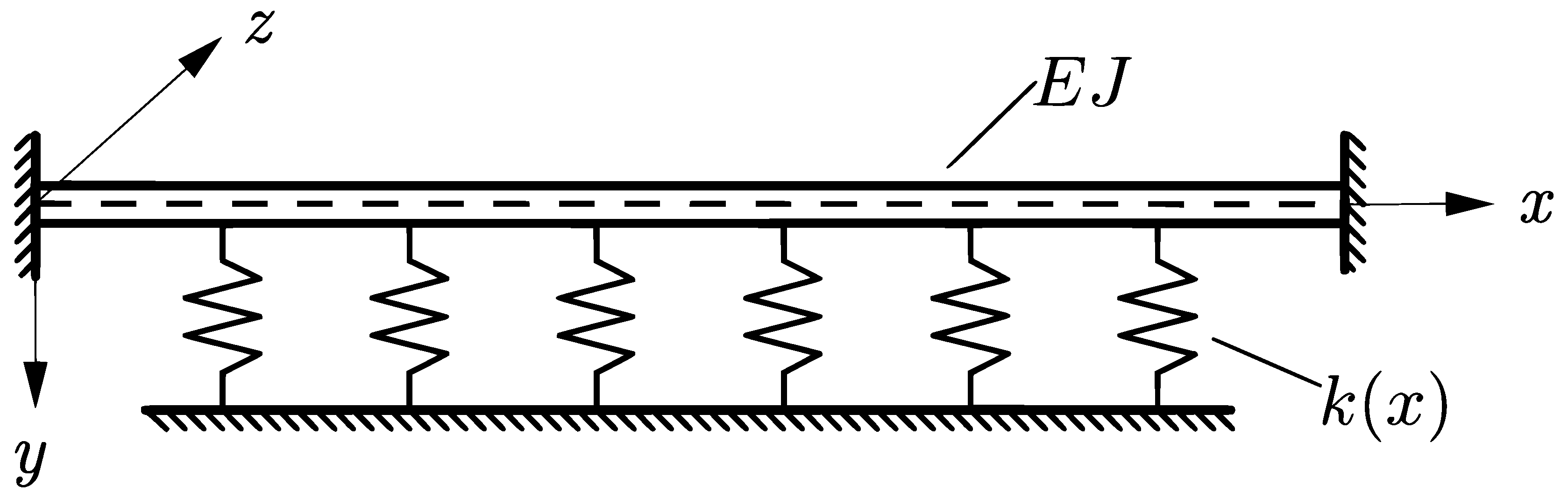
Consider a beam of unit length endowed with a right-handed system of rectangular coordinates $(x,y,z)$ with the origin at the center of gravity of the left cross-section of the beam; the x-axis is taken along the axis of the beam, while the y- and z-axes are taken along the principal axis of cross section, the positive direction of the y-axis being oriented vertically downward (see Figure 1).

The equation of free transverse vibrations of a beam of length $l=1$ has the following form:

$$\rho A\frac{{\partial }^{2}w(x,t)}{\partial t^2}+k\left(x\right)w(x,t)+EJ\frac{{\partial }^{4}w(x,t)}{\partial x^4}=0,$$

where $\rho$ is the density of material, $(\mathrm{kg}\hspace{0.17em}{\mathrm{m}}^{-3})$; A is the cross-sectional area, $\left({\mathrm{m}}^2\right)$; E is the elastic modulus of material, $(\mathrm{N}\hspace{0.17em}{\mathrm{m}}^{-2})$; J is the moment of inertia of the cross-sectional area of relative to around the z axis, $\left({\mathrm{m}}^4\right)$.

The problem of transverse vibrations of a beam of unit length after replacement $w(x,t)=v(\lambda ,x)sin\left(\omega t\right)$ reduces to the following spectral problem:

$$EJ{v}^{IV}(\lambda ,x)+k\left(x\right)v(\lambda ,x)=\lambda v(\lambda ,x),x\in I_p,p=1,2$$

(1)

where $v(\lambda ,x)$ are the eigenfunctions of the transverse static deflection of the beam; $\lambda =\rho A{\omega }^2$ are the eigenvalues, $\omega$ are the frequency parameters, $\left(\mathrm{Hz}\right)$; $I_p$ are the finite intervals. In this study, the bending stiffness, $EJ$, is assumed to be a constant; such a beam is called uniform. We present the necessary boundary conditions on finite intervals and their physical interpretations for convenience of presentation in

Table 1. The types of boundary conditions on the finite intervals and their interpretations.

Intervals	The Physical Interpretation	The Types of the Boundary Conditions	Number of Conditions
$$I_1=(0,1)$$	Clamped-clamped at the points $x=0,x=1$	$v(\lambda ,0)=0,v^{\prime }(\lambda ,0)=0,$$v(\lambda ,1)=0,v^{\prime }(\lambda ,1)=0$	(2)
$$I_2=\left(\frac{1}{2},1\right)$$	Sliding at the point $x=\frac{1}{2}$, Clamped at the point $x=1$	$v^{\prime }\left(\lambda ,\frac{1}{2}\right)=0,v^{\prime \prime \prime }\left(\lambda ,\frac{1}{2}\right)=0,$$v(\lambda ,1)=0,v^{\prime }(\lambda ,1)=0$	(3)
$$I_2=\left(\frac{1}{2},1\right)$$	Hinged at the point $x=\frac{1}{2}$, Clamped at the point $x=1$	$v\left(\lambda ,\frac{1}{2}\right)=0,v^{\prime \prime }\left(\lambda ,\frac{1}{2}\right)=0$ , $v(\lambda ,1)=0,v^{\prime }(\lambda ,1)=0$	(4)
$$I_1=(0,1)$$	Hinged-hinged at the points $x=0,x=1$	$v(\lambda ,0)=0,v^{\prime \prime }(\lambda ,0)=0,$$v(\lambda ,1)=0,v^{\prime \prime }(\lambda ,1)=0$	(5)
$$I_2=\left(\frac{1}{2},1\right)$$	Sliding at the point $x=\frac{1}{2}$, Hinged at the point $x=1$	$v^{\prime }\left(\lambda ,\frac{1}{2}\right)=0,v^{\prime \prime \prime }\left(\lambda ,\frac{1}{2}\right)=0,$$v(\lambda ,1)=0,v^{\prime \prime }(\lambda ,1)=0$	(6)
$$I_2=\left(\frac{1}{2},1\right)$$	Hinged at the point $x=\frac{1}{2}$, Hinged at the point $x=1$	$v\left(\lambda ,\frac{1}{2}\right)=0,v^{\prime \prime }\left(\lambda ,\frac{1}{2}\right)=0$ , $v(\lambda ,1)=0,v^{\prime \prime }(\lambda ,1)=0$	(7)
$$I_1=(0,1)$$	Free-free at the points $x=0,x=1$	$v^{\prime \prime }(\lambda ,0)=0,v^{\prime \prime \prime }(\lambda ,0)=0,$$v^{\prime \prime }(\lambda ,1)=0,v^{\prime \prime \prime }(\lambda ,1)=0$	(8)
$$I_2=\left(\frac{1}{2},1\right)$$	Sliding at the point $x=\frac{1}{2}$, Free at the point $x=1$	$v^{\prime }\left(\lambda ,\frac{1}{2}\right)=0,v^{\prime \prime \prime }\left(\lambda ,\frac{1}{2}\right)=0,$$v^{\prime \prime }(\lambda ,1)=0,v^{\prime \prime \prime }(\lambda ,1)=0$	(9)
$$I_2=\left(\frac{1}{2},1\right)$$	Hinged at the point $x=\frac{1}{2}$, Free at the point $x=1$	$v\left(\lambda ,\frac{1}{2}\right)=0,v^{\prime \prime }\left(\lambda ,\frac{1}{2}\right)=0$ , $v^{\prime \prime }(\lambda ,1)=0,v^{\prime \prime \prime }(\lambda ,1)=0$	(10)

(see [27,28,29]).

The main question of this work is to study the characteristics and the connections of the set of eigenvalues and eigenfunctions of the fourth order differential equation with a variable coefficient in Equation (1) with two-point boundary conditions in Equations (2), (5) and (8).

2.1. Clamped-Clamped Euler–Bernoulli Beam

First, consider the behavior of the eigenvalues of the clamped-clamped Euler–Bernoulli beam. Let $\sigma \left(A_1\right),\sigma \left(B_1\right),\sigma \left(C_1\right)$ be a set of eigenvalues of problems $A_1-\lambda I,$$B_1-\lambda I,$$C_1-\lambda I$ generated by Equation (1) on finite intervals by boundary conditions in Equations (2)–(4), respectively; the data are shown in Table 1.

Main results. The first result of the work is

Theorem 1.

Let $k\left(x\right)$ be a symmetric function with respect to the point $x=\frac{1}{2}$:

$$k\left(x\right)=k(1-x),x\in [0;1].$$

(11)

The following statements are true:

1.

$\sigma \left(A_1\right)\equiv \sigma \left(B_1\right)\cup \sigma \left(C_1\right)$

2.

If $\lambda \in \sigma \left(B_1\right)$ or $\lambda \in \sigma \left(C_1\right)$, then the eigenfunctions of problems $A-\lambda I$ corresponding to the eigenvalues λ are symmetric or asymmetric with respect to the middle of the beam at the point $x=\frac{1}{2}$ on the interval $(0,1)$, respectively.

An essential role is played by the following assertion.

Lemma 1.

Let the function $k\left(x\right)$ satisfy the condition of Equation (11). Then, there exists a fundamental system $\left\{v_i(\lambda ,x)\right\}$, $(i=\overline{1,4})$ of solutions of Equation (1) where two solutions are symmetric and two other solutions are asymmetric around the point $x=\frac{1}{2}$ on the segment $[0,1]$, i.e.,

$$v_i(\lambda ,x)={\left(-1\right)}^{i+1}{v}_i(\lambda ,1-x),(i=\overline{1,4})x\in \left[\frac{1}{2},1\right].$$

(12)

Proof of Lemma 1.

Consider the Cauchy problem with the zero initial conditions at the point $x=\frac{1}{2}$ for the function $w(\lambda ,x)=v(\lambda ,x)-\alpha v(\lambda ,1-x)$. The initial conditions acquire the form

$$w^{(i-1)}\left(\lambda ,\frac{1}{2}\right)=\left(1-{\left(-1\right)}^{i-1}\alpha \right)v^{(i-1)}\left(\lambda ,\frac{1}{2}\right)=0,(i=\overline{1,4})$$

(13)

From Equation (13), it follows that the first and third derivatives of any symmetric $(\alpha =1)$ solution $w_{+}(\lambda ,x)$ of Equation (1), as well as any asymmetric $(\alpha =-1)$ solution $w_{-}(\lambda ,x)$ together with its second derivative, are zero at the point $x=\frac{1}{2}$. In particular, these properties hold for the fundamental system of solutions $\left\{v_i(\lambda ,x)\right\},(i=\overline{1,4})$, generated by the following conditions at the point $x=\frac{1}{2}$:

$${\left.v_i^{(s-1)}(\lambda ,x)\right|}_{x=\frac{1}{2}}=\left\{\begin{array}{cc}0,& ifi\ne s\\ 1,& ifi=s,\end{array},i,s=\overline{1,4}.\right.$$

(14)

Thus, when the condition of symmetry of Equation (11) is satisfied, there are two symmetric $\left\{v_1(\lambda ,x),v_3(\lambda ,x)\right\}$ and two asymmetric $\left\{v_2(\lambda ,x),v_4(\lambda ,x)\right\}$ fundamental solutions. Note that the existence of a fundamental system of solutions at an arbitrary point $x_0\in [0,1]$ for Equation (1) was proved in [30].

The proof is complete. □

Proof of Theorem 1.

We show correctness of the relation ${\Delta }_{A_1}\left(\lambda \right)={\Delta }_{B_1}\left(\lambda \right)·{\Delta }_{C_1}\left(\lambda \right)$ for proving of Statement 1, where ${\Delta }_{A_1}\left(\lambda \right),$${\Delta }_{B_1}\left(\lambda \right),$${\Delta }_{C_1}\left(\lambda \right)$ are the characteristic determinants of correspond problems $A_1-\lambda I,B_1-\lambda I,C_1-\lambda I$.

Let $\left\{v_i(\lambda ,x)\right\},(i=\overline{1,4)}$ be a fundamental system of solutions generated by the conditions of Equation (14). Then, we get the characteristic determinant as [30] (pp. 1–27)

$${\Delta }_{A_1}\left(\lambda \right)=\left|\begin{array}{cccc}{v}_1(\lambda ,0)& v_2(\lambda ,0)& v_3(\lambda ,0)& v_4(\lambda ,0)\\ v_1^{\prime }(\lambda ,0)& v_2^{\prime }(\lambda ,0)& v_3^{\prime }(\lambda ,0)& v_4^{\prime }(\lambda ,0)\\ v_1(\lambda ,1)& v_2(\lambda ,1)& v_3(\lambda ,1)& v_4(\lambda ,1)\\ v_1^{\prime }(\lambda ,1)& v_2^{\prime }(\lambda ,1)& v_3^{\prime }(\lambda ,1)& v_4^{\prime }(\lambda ,1)\end{array}\right|$$

Taking the relation in Equation (12) into account, the characteristic determinant ${\Delta }_{A_1}\left(\lambda \right)$ can be rewritten in the following form:

$${\Delta }_{A_1}\left(\lambda \right)=\left|\begin{array}{cc}{v}_1(\lambda ,1)& v_3(\lambda ,1)\\ v_1^{\prime }(\lambda ,1)& v_3^{\prime }(\lambda ,1)\end{array}\right|·\left|\begin{array}{cc}{v}_2(\lambda ,1)& v_4(\lambda ,1)\\ v_2^{\prime }(\lambda ,1)& v_4^{\prime }(\lambda ,1)\end{array}\right|$$

(15)

The characteristic determinants of the problems $B_1-\lambda I$ and $C_1-\lambda I$ are obtained by direct substitution and by taking Equation (14) into account in the following form:

$${\Delta }_{B_1}\left(\lambda \right)=\left|\begin{array}{cc}{v}_1(\lambda ,1)& v_3(\lambda ,1)\\ v_1^{\prime }(\lambda ,1)& v_3^{\prime }(\lambda ,1)\end{array}\right|,\hspace{1em}{\Delta }_{C_1}\left(\lambda \right)=\left|\begin{array}{cc}{v}_2(\lambda ,1)& v_4(\lambda ,1)\\ v_2^{\prime }(\lambda ,1)& v_4^{\prime }(\lambda ,1)\end{array}\right|,$$

From the relation ${\Delta }_{A_1}\left(\lambda \right)={\Delta }_{B_1}\left(\lambda \right)·{\Delta }_{C_1}\left(\lambda \right)$, the proof of Statement 1 of Theorem 1 follows.

Proof of Statement 2. The general solution of Equation (1) has the following form:

$$v(\lambda ,x)={\sum }_{i=1}^4{d}_i{\tilde{v}}_i(\lambda ,x)$$

for the interval $\left(\frac{1}{2},1\right)$. Here, $\left\{{\tilde{v}}_i(\lambda ,x)\right\},(i=1,2,3,4)$ are the fundamental system of solutions of Equation (1) given by the conditions in Equation (14) on the interval $\left(\frac{1}{2},1\right)$. Let ${\lambda }^{\prime }\in {\sigma }_{B_1}\left(\lambda \right)$ be the eigenvalues; then, a linear combination of the fundamental solutions

$${\tilde{v}}_{+}({\lambda }^{\prime },x)=d_1{\tilde{v}}_1({\lambda }^{\prime },x)+d_3{\tilde{v}}_3({\lambda }^{\prime },x)$$

is the solution of Equation (1) and satisfies the condition in Equation (3):

$${\tilde{v}}_{+}^{\prime }\left({\lambda }^{\prime },\frac{1}{2}\right)=0,{\tilde{v}}_{+}^{\prime \prime \prime }\left({\lambda }^{\prime },\frac{1}{2}\right)=0$$

$${\tilde{v}}_{+}({\lambda }^{\prime },1)=0,{\tilde{v}}_{+}^{\prime }({\lambda }^{\prime },1)=0$$

This function is the eigenfunction of problem $B_1-\lambda I$ on the interval $\left(\frac{1}{2},1\right)$. Moreover, its characteristic determinant is given by the formula

$${\Delta }_{B_1}\left(\lambda \right)=\left|\begin{array}{cc}{\tilde{v}}_1({\lambda }^{\prime },1)& {\tilde{v}}_3({\lambda }^{\prime },1)\\ {\tilde{v}}_1^{\prime }({\lambda }^{\prime },1)& {\tilde{v}}_3^{\prime }({\lambda }^{\prime },1)\end{array}\right|.$$

The functions ${\tilde{v}}_{+}({\lambda }^{\prime },x)$, ${\tilde{v}}_1({\lambda }^{\prime },x)$ and ${\tilde{v}}_3({\lambda }^{\prime },x)$ will continue symmetrically on the interval $\left(0,\frac{1}{2}\right)$ if the condition of symmetry, Equation (11), is satisfied and if the Lemma 1 is taken into account. These are denoted as $v_{+}({\lambda }^{\prime },x)$, $v_1({\lambda }^{\prime },x)$ and $v_3({\lambda }^{\prime },x)$, respectively. Furthermore, we consider these functions on the entire interval $(0,1)$. The conditions at the point $x=1$ are satisfied automatically for $v_{+}({\lambda }^{\prime },x)$. Verification is required only for the conditions at the point $x=0$:

$$v_{+}({\lambda }^{\prime },0)=0,v_{+}^{\prime }({\lambda }^{\prime },0)=0$$

(16)

Substituting $v_{+}({\lambda }^{\prime },x)$ into the condition in Equation (16), the characteristic determinant is obtained as:

$$\left|\begin{array}{cc}{v}_1({\lambda }^{\prime },0)& v_3({\lambda }^{\prime },0)\\ v_1^{\prime }({\lambda }^{\prime },0)& v_3^{\prime }({\lambda }^{\prime },0)\end{array}\right|.$$

Taking the symmetry of the solutions $v_1({\lambda }^{\prime },x)$, $v_3({\lambda }^{\prime },x)$ into account with respect to $x=\frac{1}{2}$, this expression can be reduced to the form

$$\left|\begin{array}{cc}{v}_1({\lambda }^{\prime },1)& v_3({\lambda }^{\prime },1)\\ v_1^{\prime }({\lambda }^{\prime },1)& v_3^{\prime }({\lambda }^{\prime },1)\end{array}\right|={\Delta }_{B_1}\left({\lambda }^{\prime }\right).$$

Since ${\lambda }^{\prime }$ is a zero of ${\Delta }_{B_1}\left(\lambda \right)$, from representation in Equation (15), it follows that it is a zero of ${\Delta }_{A_1}\left(\lambda \right)$. Thus, the execution of the condition in Equation (16) is proved. Therefore, the continued function $v_{+}({\lambda }^{\prime },x)$ is the eigenfunction of the operator $A_1-{\lambda }^{\prime }I$ on the interval $(0,1)$. The second part of Statement 2 will be proved similarly.

The proof is complete. □

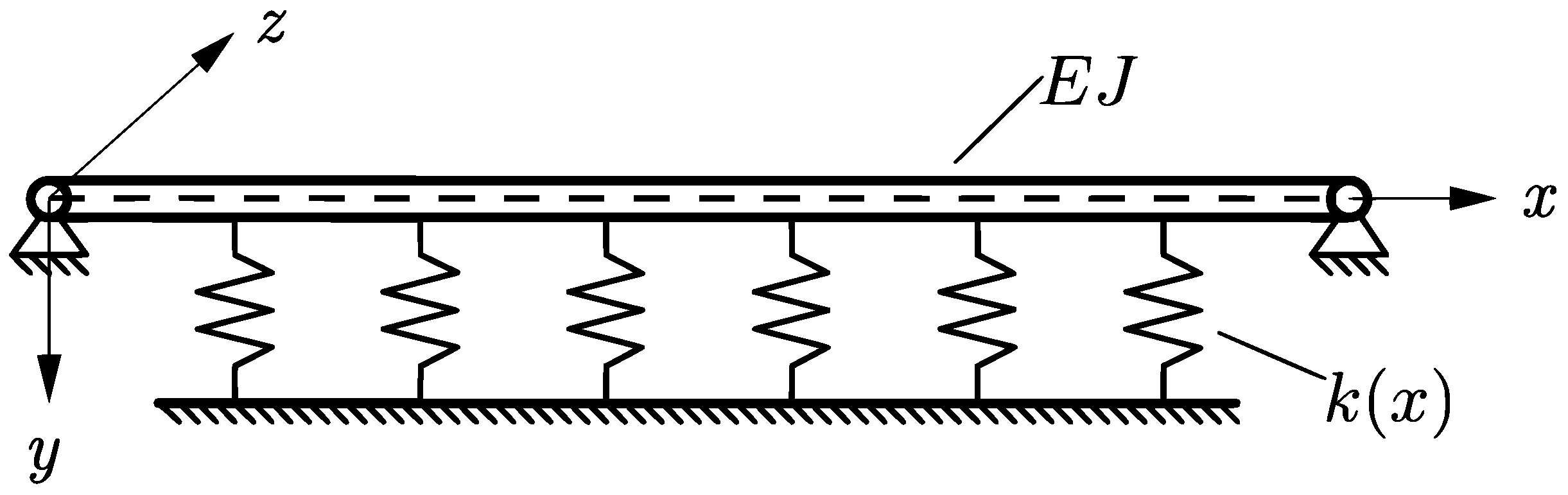
2.2. Hinged-Hinged Euler–Bernoulli Beam

Consider the behavior of the eigenvalues of the hinged-hinged Euler–Bernoulli beam (see Figure 2). Let $\sigma \left(A_2\right),\sigma \left(B_2\right),\sigma \left(C_2\right)$ be a set of eigenvalues of problems $A_2-\lambda I,$ $B_2-\lambda I,$ $C_2-\lambda I$ generated by Equation (1) on finite intervals by boundary conditions in Equations (5)–(7), respectively; the data are shown in Table 1.

Theorem 2.

Let $k\left(x\right)$ be a symmetric function with respect to the point $x=\frac{1}{2},$ i.e., the condition in Equation (11) holds. The following statements are true:

1.

$\sigma \left(A_2\right)\equiv \sigma \left(B_2\right)\cup \sigma \left(C_2\right)$

2.

If $\lambda \in \sigma \left(B_2\right)$ or $\lambda \in \sigma \left(C_2\right)$, then the eigenfunctions of problems $A_2-\lambda I$ corresponding to the eigenvalues λ are symmetric or asymmetric with respect to the middle of the beam at the point $x=\frac{1}{2}$ on the interval $(0,1)$, respectively.

Proof of Theorem 2.

We show correctness of the relation ${\Delta }_{A_2}\left(\lambda \right)={\Delta }_{B_2}\left(\lambda \right)·{\Delta }_{C_2}\left(\lambda \right)$ for proving of Statement 1, where ${\Delta }_{A_2}\left(\lambda \right),$ ${\Delta }_{B_2}\left(\lambda \right),$ ${\Delta }_{C_2}\left(\lambda \right)$ are the characteristic determinants of correspond problems $A_2-\lambda I,B_2-\lambda I,C_2-\lambda I$.

Let $\left\{v_i(\lambda ,x)\right\},(i=\overline{1,4})$ be a fundamental system of solutions generated by the conditions in Equation (7). Then, we get the characteristic determinant as [30] (pp. 1–27):

$${\Delta }_{A_2}\left(\lambda \right)=\left|\begin{array}{cccc}{v}_1(\lambda ,0)& v_2(\lambda ,0)& v_3(\lambda ,0)& v_4(\lambda ,0)\\ v_1^{\prime \prime }(\lambda ,0)& v_2^{\prime \prime }(\lambda ,0)& v_3^{\prime \prime }(\lambda ,0)& v_4^{\prime \prime }(\lambda ,0)\\ v_1(\lambda ,1)& v_2(\lambda ,1)& v_3(\lambda ,1)& v_4(\lambda ,1)\\ v_1^{\prime \prime }(\lambda ,1)& v_2^{\prime \prime }(\lambda ,1)& v_3^{\prime \prime }(\lambda ,1)& v_4^{\prime \prime }(\lambda ,1)\end{array}\right|$$

Taking the relation in Equation (12) into account, the characteristic determinant ${\Delta }_{A_2}\left(\lambda \right)$ can be rewritten in the following form:

$${\Delta }_{A_2}\left(\lambda \right)=\left|\begin{array}{cc}{v}_3(\lambda ,1)& v_1(\lambda ,1)\\ v_3^{\prime \prime }(\lambda ,1)& v_1^{\prime \prime }(\lambda ,1)\end{array}\right|·\left|\begin{array}{cc}{v}_2(\lambda ,1)& v_4(\lambda ,1)\\ v_2^{\prime \prime }(\lambda ,1)& v_4^{\prime \prime }(\lambda ,1)\end{array}\right|$$

(17)

The characteristic determinants of the problems $B_2-\lambda I$ and $C_2-\lambda I$ are obtained by direct substitution and by taking Equation (14) in the following form into account:

$${\Delta }_{B_2}\left(\lambda \right)=\left|\begin{array}{cc}{v}_3(\lambda ,1)& v_1(\lambda ,1)\\ v_3^{\prime \prime }(\lambda ,1)& v_1^{\prime \prime }(\lambda ,1)\end{array}\right|,\hspace{1em}{\Delta }_{C_2}\left(\lambda \right)=\left|\begin{array}{cc}{v}_2(\lambda ,1)& v_4(\lambda ,1)\\ v_2^{\prime \prime }(\lambda ,1)& v_4^{\prime \prime }(\lambda ,1)\end{array}\right|,$$

From the relation ${\Delta }_{A_2}\left(\lambda \right)={\Delta }_{B_2}\left(\lambda \right)·{\Delta }_{C_2}\left(\lambda \right)$, the proof of the Statement 1 of Theorem 2 follows.

Proof of the Statement 2. The general solution of Equation (1) has the following form:

$$v(\lambda ,x)={\sum }_{i=1}^4{d}_i{\tilde{v}}_i(\lambda ,x)$$

for the interval $\left(\frac{1}{2},1\right)$. Here $\left\{{\tilde{v}}_i(\lambda ,x)\right\},(i=1,2,3,4)$ are the fundamental system of solutions of Equation (1) given by the conditions in Equation (14) on the interval $\left(\frac{1}{2},1\right)$. Let ${\lambda }^{\prime }\in {\sigma }_{B_2}\left(\lambda \right)$ be the eigenvalues; then, a linear combination of the fundamental solutions

$${\tilde{v}}_{+}({\lambda }^{\prime },x)=d_1{\tilde{v}}_1({\lambda }^{\prime },x)+d_3{\tilde{v}}_3({\lambda }^{\prime },x)$$

is the solution of Equation (1) and satisfies the condition in Equation (6):

$${\tilde{v}}_{+}^{\prime }\left({\lambda }^{\prime },\frac{1}{2}\right)=0,{\tilde{v}}_{+}^{\prime \prime \prime }\left({\lambda }^{\prime },\frac{1}{2}\right)=0$$

$${\tilde{v}}_{+}({\lambda }^{\prime },1)=0,{\tilde{v}}_{+}^{\prime \prime }({\lambda }^{\prime },1)=0$$

This function is the eigenfunction of problem $B_2-\lambda I$ on the interval $\left(\frac{1}{2},1\right)$. Moreover, its characteristic determinant is given by the formula

$${\Delta }_{B_2}\left(\lambda \right)=\left|\begin{array}{cc}{\tilde{v}}_3({\lambda }^{\prime },1)& {\tilde{v}}_1({\lambda }^{\prime },1)\\ {\tilde{v}}_3^{\prime \prime }({\lambda }^{\prime },1)& {\tilde{v}}_1^{\prime \prime }({\lambda }^{\prime },1)\end{array}\right|.$$

The functions ${\tilde{v}}_{+}({\lambda }^{\prime },x)$, ${\tilde{v}}_1({\lambda }^{\prime },x)$ and ${\tilde{v}}_3({\lambda }^{\prime },x)$ will continue symmetrically on the interval $\left(0,\frac{1}{2}\right)$ if the condition of symmetry in Equation (11) is satisfied and if the Lemma 1 is take into account. These are denoted as $v_{+}({\lambda }^{\prime },x)$, $v_1({\lambda }^{\prime },x)$ and $v_3({\lambda }^{\prime },x)$, respectively. Furthermore, we consider these functions on the entire interval $(0,1)$. The conditions at the point $x=1$ are satisfied automatically for $v_{+}({\lambda }^{\prime },x)$. Verification is required only for the conditions at the point $x=0$:

$$v_{+}({\lambda }^{\prime },0)=0,v_{+}^{\prime \prime }({\lambda }^{\prime },0)=0$$

(18)

Substituting $v_{+}({\lambda }^{\prime },x)$ into the condition in Equation (18), the characteristic determinant is obtained as:

$$\left|\begin{array}{cc}{v}_3({\lambda }^{\prime },0)& v_1({\lambda }^{\prime },0)\\ v_3^{\prime \prime }({\lambda }^{\prime },0)& v_1^{\prime \prime }({\lambda }^{\prime },0)\end{array}\right|.$$

Taking the symmetry of the solutions $v_1({\lambda }^{\prime },x)$, $v_3({\lambda }^{\prime },x)$ into account with respect to $x=\frac{1}{2}$, this expression can be reduced to the form

$$\left|\begin{array}{cc}{v}_3({\lambda }^{\prime },1)& v_1({\lambda }^{\prime },1)\\ v_3^{\prime \prime }({\lambda }^{\prime },1)& v_1^{\prime \prime }({\lambda }^{\prime },1)\end{array}\right|={\Delta }_{B_2}\left({\lambda }^{\prime }\right).$$

Since ${\lambda }^{\prime }$ is a zero of ${\Delta }_{B_2}\left(\lambda \right),$ from representation in Equation (17), it follows that it is a zero of ${\Delta }_{A_2}\left(\lambda \right)$. Thus, the execution of the condition in Equation (18) is proved. Therefore, the continued function $v_{+}({\lambda }^{\prime },x)$ is the eigenfunction of the operator $A_2-{\lambda }^{\prime }I$ on the interval $(0,1)$. The second part of Statement 2 will be proved similarly.

The proof is complete. □

2.3. Free-Free Euler–Bernoulli Beam

Consider the behavior of the eigenvalues of the free-free Euler–Bernoulli beam (see Figure 3). Let $\sigma \left(A_3\right),\sigma \left(B_3\right),\sigma \left(C_3\right)$ be a set of eigenvalues of problems $A_3-\lambda I,$ $B_3-\lambda I,$ $C_3-\lambda I$ generated by Equation (1) on finite intervals by the boundary conditions in Equations (8)–(10), respectively; the data are shown in Table 1.

Theorem 3.

Let $k\left(x\right)$ be a symmetric function with respect to the point $x=\frac{1}{2},$ i.e., the condition in Equation (11) holds. The following statements are true:

1.

$\sigma \left(A_3\right)\equiv \sigma \left(B_3\right)\cup \sigma \left(C_3\right)$

2.

If $\lambda \in \sigma \left(B_3\right)$ or $\lambda \in \sigma \left(C_3\right)$, then the eigenfunctions of problems $A_3-\lambda I$ corresponding to the eigenvalues λ are symmetric or asymmetric with respect to the middle of the beam at the point $x=\frac{1}{2}$ on the interval $(0,1)$ respectively.

Proof of Theorem 3.

We show correctness of the relation ${\Delta }_{A_3}\left(\lambda \right)={\Delta }_{B_3}\left(\lambda \right)·{\Delta }_{C_3}\left(\lambda \right)$ for proving of Statement 1, where ${\Delta }_{A_3}\left(\lambda \right),$ ${\Delta }_{B_3}\left(\lambda \right),$ ${\Delta }_{C_3}\left(\lambda \right)$ are the characteristic determinants of corresponding problems $A_3-\lambda I,B_3-\lambda I,C_3-\lambda I$.

Let $\left\{v_i(\lambda ,x)\right\},(i=\overline{1,4})$ be a fundamental system of solutions generated by the conditions in Equation (14). Then, we get the characteristic determinant as [30] (pp. 1–27):

$${\Delta }_{A_3}\left(\lambda \right)=\left|\begin{array}{cccc}{v}_1^{\prime \prime }(\lambda ,0)& v_2^{\prime \prime }(\lambda ,0)& v_3^{\prime \prime }(\lambda ,0)& v_4^{\prime \prime }(\lambda ,0)\\ v_1^{\prime \prime \prime }(\lambda ,0)& v_2^{\prime \prime \prime }(\lambda ,0)& v_3^{\prime \prime \prime }(\lambda ,0)& v_4^{\prime \prime \prime }(\lambda ,0)\\ v_1^{\prime \prime }(\lambda ,1)& v_2^{\prime \prime }(\lambda ,1)& v_3^{\prime \prime }(\lambda ,1)& v_4^{\prime \prime }(\lambda ,1)\\ v_1^{\prime \prime \prime }(\lambda ,1)& v_2^{\prime \prime \prime }(\lambda ,1)& v_3^{\prime \prime \prime }(\lambda ,1)& v_4^{\prime \prime \prime }(\lambda ,1)\end{array}\right|$$

Taking the relation in Equation (12) into account, the characteristic determinant ${\Delta }_{A_3}\left(\lambda \right)$ can be rewritten in the following form:

$${\Delta }_{A_3}\left(\lambda \right)=\left|\begin{array}{cc}{v}_1^{\prime \prime \prime }(\lambda ,1)& v_3^{\prime \prime \prime }(\lambda ,1)\\ v_1^{\prime \prime }(\lambda ,1)& v_3^{\prime \prime }(\lambda ,1)\end{array}\right|·\left|\begin{array}{cc}{v}_2^{\prime \prime \prime }(\lambda ,1)& v_4^{\prime \prime \prime }(\lambda ,1)\\ v_2^{\prime \prime }(\lambda ,1)& v_4^{\prime \prime }(\lambda ,1)\end{array}\right|$$

(19)

The characteristic determinants of the problems $B_3-\lambda I$ and $C_3-\lambda I$ are obtained by direct substitution and by taking Equation (14) in the following form into account:

$${\Delta }_{B_3}\left(\lambda \right)=\left|\begin{array}{cc}{v}_1^{\prime \prime \prime }(\lambda ,1)& v_3^{\prime \prime \prime }(\lambda ,1)\\ v_1^{\prime \prime }(\lambda ,1)& v_3^{\prime \prime }(\lambda ,1)\end{array}\right|,\hspace{1em}{\Delta }_{C_3}\left(\lambda \right)=\left|\begin{array}{cc}{v}_2^{\prime \prime \prime }(\lambda ,1)& v_4^{\prime \prime \prime }(\lambda ,1)\\ v_2^{\prime \prime }(\lambda ,1)& v_4^{\prime \prime }(\lambda ,1)\end{array}\right|,$$

From the relation ${\Delta }_{A_3}\left(\lambda \right)={\Delta }_{B_3}\left(\lambda \right)·{\Delta }_{C_3}\left(\lambda \right)$, the proof of Statement 1 of Theorem 3 follows. □

Proof of the Statement 2.

The general solution of Equation (1) has the following form:

$$v(\lambda ,x)={\sum }_{i=1}^4{d}_i{\tilde{v}}_i(\lambda ,x)$$

for the interval $\left(\frac{1}{2},1\right)$. Here, $\left\{{\tilde{v}}_i(\lambda ,x)\right\},(i=\overline{1,4})$ are the fundamental system of solutions of Equation (1) given by the conditions in Equation (14) on the interval $\left(\frac{1}{2},1\right)$. Let ${\lambda }^{\prime }\in {\sigma }_{B_3}\left(\lambda \right)$ be the eigenvalues; then, a linear combination of the fundamental solutions

$${\tilde{v}}_{+}({\lambda }^{\prime },x)=d_1{\tilde{v}}_1({\lambda }^{\prime },x)+d_3{\tilde{v}}_3({\lambda }^{\prime },x)$$

is the solution of Equation (1) and satisfies the condition in Equation (9):

$${\tilde{v}}_{+}^{\prime }\left({\lambda }^{\prime },\frac{1}{2}\right)=0,{\tilde{v}}_{+}^{\prime \prime \prime }\left({\lambda }^{\prime },\frac{1}{2}\right)=0$$

$${\tilde{v}}_{+}^{\prime \prime }({\lambda }^{\prime },1)=0,{\tilde{v}}_{+}^{\prime \prime \prime }({\lambda }^{\prime },1)=0$$

This function is the eigenfunction of problem $B_3-\lambda I$ on the interval $\left(\frac{1}{2},1\right)$. Moreover, its characteristic determinant is given by the formula

$${\Delta }_{B_3}\left(\lambda \right)=\left|\begin{array}{cc}{\tilde{v}}_1^{\prime \prime \prime }({\lambda }^{\prime },1)& {\tilde{v}}_3^{\prime \prime \prime }({\lambda }^{\prime },1)\\ {\tilde{v}}_1^{\prime \prime }({\lambda }^{\prime },1)& {\tilde{v}}_3^{\prime \prime }({\lambda }^{\prime },1)\end{array}\right|.$$

The functions ${\tilde{v}}_{+}({\lambda }^{\prime },x)$, ${\tilde{v}}_1({\lambda }^{\prime },x)$ and ${\tilde{v}}_3({\lambda }^{\prime },x)$ will continue symmetrically on the interval $\left(0,\frac{1}{2}\right)$ if the condition of symmetry in Equation (11) is satisfied and if Lemma 1 is taken into account. These are denoted as $v_{+}({\lambda }^{\prime },x)$, $v_1({\lambda }^{\prime },x)$ and $v_3({\lambda }^{\prime },x)$, respectively. Furthermore, we consider these functions on the entire interval $(0,1)$. The conditions at the point $x=1$ are satisfied automatically for $v_{+}({\lambda }^{\prime },x)$. Verification is required only for the conditions at the point $x=0$:

$$v_{+}^{\prime \prime }({\lambda }^{\prime },0)=0,v_{+}^{\prime \prime \prime }({\lambda }^{\prime },0)=0$$

(20)

Substituting $v_{+}({\lambda }^{\prime },x)$ into the condition in Equation (20), the characteristic determinant is obtained as:

$$\left|\begin{array}{cc}{v}_1^{\prime \prime \prime }({\lambda }^{\prime },0)& v_3^{\prime \prime \prime }({\lambda }^{\prime },0)\\ v_1^{\prime \prime }({\lambda }^{\prime },0)& v_3^{\prime \prime }({\lambda }^{\prime },0)\end{array}\right|.$$

Taking the symmetry of the solutions $v_1({\lambda }^{\prime },x)$, $v_3({\lambda }^{\prime },x)$ into account with respect to $x=\frac{1}{2}$, this expression can be reduced to the form

$$\left|\begin{array}{cc}{v}_1^{\prime \prime \prime }({\lambda }^{\prime },1)& v_3^{\prime \prime \prime }({\lambda }^{\prime },1)\\ v_1^{\prime \prime }({\lambda }^{\prime },1)& v_3^{\prime \prime }({\lambda }^{\prime },1)\end{array}\right|={\Delta }_{B_3}\left({\lambda }^{\prime }\right).$$

Since ${\lambda }^{\prime }$ is a zero of ${\Delta }_{B_3}\left(\lambda \right)$, from the representation in Equation (19), it follows that it is a zero of ${\Delta }_{A_3}\left(\lambda \right)$. Thus, the execution of the condition in Equation (20) is proved. Therefore, the continued function $v_{+}({\lambda }^{\prime },x)$ is the eigenfunction of the operator $A_3-{\lambda }^{\prime }I$ on the interval $(0,1)$. The second part of Statement 2 will be proved similarly.

The proof is complete. □

3. Examples

In this section, we calculate approximately the five eigenvalues of boundary value problems $A_i-\lambda I,$ $B_i-\lambda I,$ $C_i-\lambda I$ $(i=1,2,3)$ generated by the Euler–Bernoulli equation for the various coefficients $k\left(x\right)$. The results of calculation of the eigenvalues are shown in the corresponding columns of

Table 2. The numerical results of first five eigenvalues for Example 1.

Clamped-Clamped at the Points $\mathit{x}=0,$ $\mathit{x}=1$	Sliding at the Point $\mathit{x}=\frac{1}{2},$ Clamped at the Point $\mathit{x}=1$	Hinged at the Point $\mathit{x}=\frac{1}{2},$ Clamped at the Point $\mathit{x}=1$
500.56	500.56	3803.53
3803.53	14,617.63	39,943.79
14,617.63	89,135.41	173,881.32
39,943.79	308,208.45	508,481.54
89,135.41	793,403.13	$1.184\times {10}^6$

,

Table 3. The numerical results of the first five eigenvalues for Example 2.

Clamped-Clamped at the Points $\mathit{x}=0,$ $\mathit{x}=1$	Sliding at the Point $\mathit{x}=\frac{1}{2},$ Clamped at the Point $\mathit{x}=1$	Hinged at the Point $\mathit{x}=\frac{1}{2},$ Clamped at the Point $\mathit{x}=1$
509.69	509.69	3811.41
3811.41	14,624.97	39,950.9
14,624.97	89,142.37	173,888.2
39,950.9	308,215.28	508,488.34
89,142.37	793,412.99	$1.184\times {10}^6$

,

Table 4. The numerical results of first five eigenvalues for Example 3.

Hinged-Hinged at the Points $\mathit{x}=0,$ $\mathit{x}=1$	Sliding at the Point $\mathit{x}=\frac{1}{2},$ Hinged at the Point $\mathit{x}=1$	Hinged at the Point $\mathit{x}=\frac{1}{2},$ Hinged at the Point $\mathit{x}=1$
97.63	97.63	1558.72
1558.72	7890.31	24,936.9
7890.31	60,880.85	126,242.35
24,936.9	233,879.4	398,987.81
60,880.85	639,101.62	974,094.13

and

Table 5. The numerical results of first five eigenvalues for Example 4.

Hinged-Hinged at the Points $\mathit{x}=0,$ $\mathit{x}=1$	Sliding at the Point $\mathit{x}=\frac{1}{2},$ Hinged at the Point $\mathit{x}=1$	Hinged at the Point $\mathit{x}=\frac{1}{2},$ Hinged at the Point $\mathit{x}=1$
99.15	97.94	1558.76
1560.86	7890.49	24,937.01
7899.55	60,881.01	126,242.48
24,939.18	233,879.54	398,987.94
60,883.15	639,101.76	974,094.28

.

Example 1.

Let $k\left(x\right)\equiv 0$ and $EJ=1.$

The numerical results of first five eigenvalues for Example 1 are shown in Table 2.

Example 2.

Let $k\left(x\right)=4x(1-x)$ and $EJ=1.$

The numerical results of first five eigenvalues for Example 2 are shown in Table 3. The calculations which represent in Examples 1 and 2 confirm the validity of Statement 1 of the Theorem 1 on the factorization of the set of eigenvalues. The physical interpretation of Statement 2 was given in [27] (p. 270) for $k\left(x\right)\equiv 0$.

Example 3.

Let $k\left(x\right)=4x(1-x)$ and $EJ=1.$ The function $k\left(x\right)$ satisfies the symmetry condition in Equation (11).

Example 4.

Let $k\left(x\right)=10{(1-x)}^3$ and $EJ=1.$ The function $k\left(x\right)$ does not satisfy the symmetry condition in Equation (11).

The violation of the regularity of factorization of eigenvalues in Example 4 is due to the asymmetry of the function $k\left(x\right).$ The above calculations in Examples 3 and 4 confirm the validity of Statement 1 of Theorem 2. The numerical results of the first five eigenvalues for Examples 3 and 4 are shown in Table 4 and Table 5, respectively.

Example 5.

Let $k\left(x\right)=10-40x(1-x)$ and $EJ=1.$ The function $k\left(x\right)$ satisfies the symmetry condition in Equation (11).

The numerical results of the first five eigenvalues for Example 5 are shown in

Table 6. The numerical results of the first five eigenvalues for Example 5.

Free-Free at the Points $\mathit{x}=0,$ $\mathit{x}=1$	Sliding at the Point $\mathit{x}=\frac{1}{2},$ Free at the Point $\mathit{x}=1$	Hinged at the Point $\mathit{x}=\frac{1}{2},$ Free at the Point $\mathit{x}=1$
3.32	3.32	5.99
5.99	505.38	3807.59
505.38	14,621.36	39,947.39
3807.59	89,138.92	173,884.78
14,621.36	308,211.88	508,484.95

. The calculations represented in Example 5 confirm the validity of Statement 1 of the Theorem 3. The eigenfunctions that confirm Statement 2 were given in [22] (Example 3.2) for $k\left(x\right)\equiv 0.$

According to the authors, the qualitative behavior of the spectrum is revealed on the basis of the qualitative theory of differential equations. In this work, numerical methods give the possibility to test hypotheses and are used as an additional tool. We used a numerical method for calculating the eigenvalues at variable coefficient of $k\left(x\right)$ with the polynomial expansion and integral techniques [25]. The degree of the polynomial was chosen $N=25$, which ensures high accuracy of calculations. Numerical calculations were carried out in the Maple computer mathematics system.

The new results can be useful for solving the inverse coefficient problems using known natural frequencies (see [31]). In the future, the practical interest will be to investigate the behavior of a beam (thermodynamic response) with a variable foundation coefficient when the beam is irradiated by moving laser pulses. This issue was investigated in [32] for the constant coefficient. The results can be generalized to investigate the dynamic design of thin films on compliant substrates [33].

4. Conclusions

In this paper, the problems for determining the eigenvalues of the uniform Euler–Bernoulli beam lying on the Winkler’s type foundation at three types of fixings at the ends were solved: clamped-clamped, hinged-hinged and free-free. The types of boundary value problems for a beam with a symmetric coefficient of foundation are described, and the set of eigenvalues on a full segment can be represented as two groups of the eigenvalues of certain problems on a half segment. If $\lambda$ belongs to the first group, the eigenfunctions of the problems on the complete segment corresponding to the eigenvalues $\lambda$ are symmetric with respect to the middle of the beam of the point $x=\frac{1}{2}$ if the second ones are asymmetric. Numerical calculations are carried out to check the validity of Statement 1 of Theorems 1–3. The proposed method can be useful for solving inverse problems of restoring the elasticity coefficient of foundation from natural frequencies and developing algorithms for nondestructive testing devices.