Multiple Lump Novel and Accurate Analytical and Numerical Solutions of the Three-Dimensional Potential Yu–Toda–Sasa–Fukuyama Equation

Abstract

The accuracy of novel lump solutions of the potential form of the three–dimensional potential Yu–Toda–Sasa–Fukuyama (3-Dp-YTSF) equation is investigated. These solutions are obtained by employing the extended simplest equation (ESE) and modified Kudryashov (MKud) schemes to explore its lump and breather wave solutions that characterizes the dynamics of solitons and nonlinear waves in weakly dispersive media, plasma physics, and fluid dynamics. The accuracy of the obtained analytical solutions is investigated through the perspective of numerical and semi-analytical strategies (septic B-spline (SBS) and variational iteration (VI) techniques). Additionally, matching the analytical and numerical solutions is represented along with some distinct types of sketches. The superiority of the MKud is showed as the fourth research paper in our series that has been beginning by Mostafa M. A. Khater and Carlo Cattani with the title “Accuracy of computational schemes”. The functioning of employed schemes appears their effectual and ability to apply to different nonlinear evolution equations.

1. Introduction

Soliton is one of the most well-known properties that characterize the integrability of nonlinear evolution equations [1,2]. Recently, the rogue waves or monster waves, freak waves, abnormal waves have been observed as one of the soliton waves which are an exceptional type of nonlinear waves that are restricted in just one direction and have much significance in a variety of physical branches [3,4]. These waves are first figured out in the deep ocean [5,6]. The applications of this wave appear in the oceanography and optical fibers [7,8,9]. Nowadays, a new branch of the rogue wave is known as a lump wave which is defined by a restricted rogue wave in every direction in space [10,11,12].

Nowadays and based on computer revolution that has a great effect on deriving computational, semi-analytical and numerical schemes, many schemes have derived such as sech-tanh expansion method, auxiliary equation method, direct algebraic equation method, iteration method, exponential expansion method, B-spline schemes, Kudryashov methods, Adomian decomposition method, Khater methods, $\left(\frac{{\phi }^{\prime }\left(\zeta \right)}{\phi \left(\zeta \right)}\right)$-expansion methods and so on [13,14,15,16,17,18,19], the lump solutions of many nonlinear phenomena have been investigated [20,21,22,23,24].

In this context, our paper aims to investigate novel lump solutions of the 3-Dp-YTSF equation through the perspective of ESE and MKud analytical techniques [25,26]. Additionally, The another goal of this manuscript limits to check semi-analytical and numerical solutions of the considered model to explain the accuracy of the obtained analytical solutions and employed analytical schemes [27,28]. The 3-Dp-YTSF equation is given by [29,30,31,32,33,34]

$$\begin{array}{c}\hfill -{\mathcal{Y}}_{xt}+{\mathcal{Y}}_{xxxz}+4{\mathcal{Y}}_x{\mathcal{Y}}_{xz}+2{\mathcal{Y}}_{xx}{\mathcal{Y}}_z+3{\mathcal{Y}}_{yy}=0.\end{array}$$

(1)

where $\mathcal{Y}=\mathcal{Y}(\zeta ,t),\zeta =(x,y,z)$ explains the dynamics of solitons and nonlinear waves. Employing the next wave transformation $\mathcal{Y}=\mathcal{Y}(x,y,z,t)=\mathcal{T}\left(\phi \right)$ where $\phi =\delta +\lambda t,\delta =x+y+z$ converts Equation (1) into the following ordinary differential equation. Integrating the obtained equation once with zero constant of integration, get

$$\begin{array}{c}\hfill (3-\lambda ){\mathcal{T}}^{\prime }+{\mathcal{T}}^{‴}+3{\left({\mathcal{T}}^{\prime }\right)}^2=0.\end{array}$$

(2)

Handling Equation (2) through the perspective of the above-mentioned analytical schemes and the homogeneous balance principles, gives $n=1$. Thus, the general solutions of Equation (2) are evaluated by

$$\begin{array}{c}\hfill \mathcal{T}\left(\phi \right)=\left\{\begin{array}{c}\sum _{i=-n}^n{a}_i\mathcal{C}{\left(\phi \right)}^i=a_1\mathcal{C}\left(\phi \right)+\frac{a_{-1}}{\mathcal{C}\left(\phi \right)}+a_0,\\ \\ \sum _{i=0}^n{a}_i\mathcal{L}{\left(\phi \right)}^i=a_1\mathcal{L}\left(\phi \right)+a_0,\end{array}\right.\end{array}$$

(3)

where $a_0,a_1,a_{-1}$ are arbitrary constants.

The structure of the other sections in this manuscript are given as follows; Section 2 investigates lump solutions of the 3-Dp-YTSF model. Additionally, checking the accuracy of the obtained solution through the above-mentioned semi-analytical and numerical schemes. Section 3 explains the obtained solutions and achieved goals of our research paper. Section 4 gives a summary of the manuscript.

2. Analytical and Numerical Matching for the 3-Dp-YTSF Equation

This section investigates the analytical, semi-analytical and numerical simulations for the 3-Dp-YTSF equation. The headline of this section can be summarized in the following order:

• Applying ESE and MKud schemes to Equation (2) to get lump wave solutions then getting the initial and boundary conditions to investigate semi-analytical and numerical solutions trough the SBS and VI techniques.
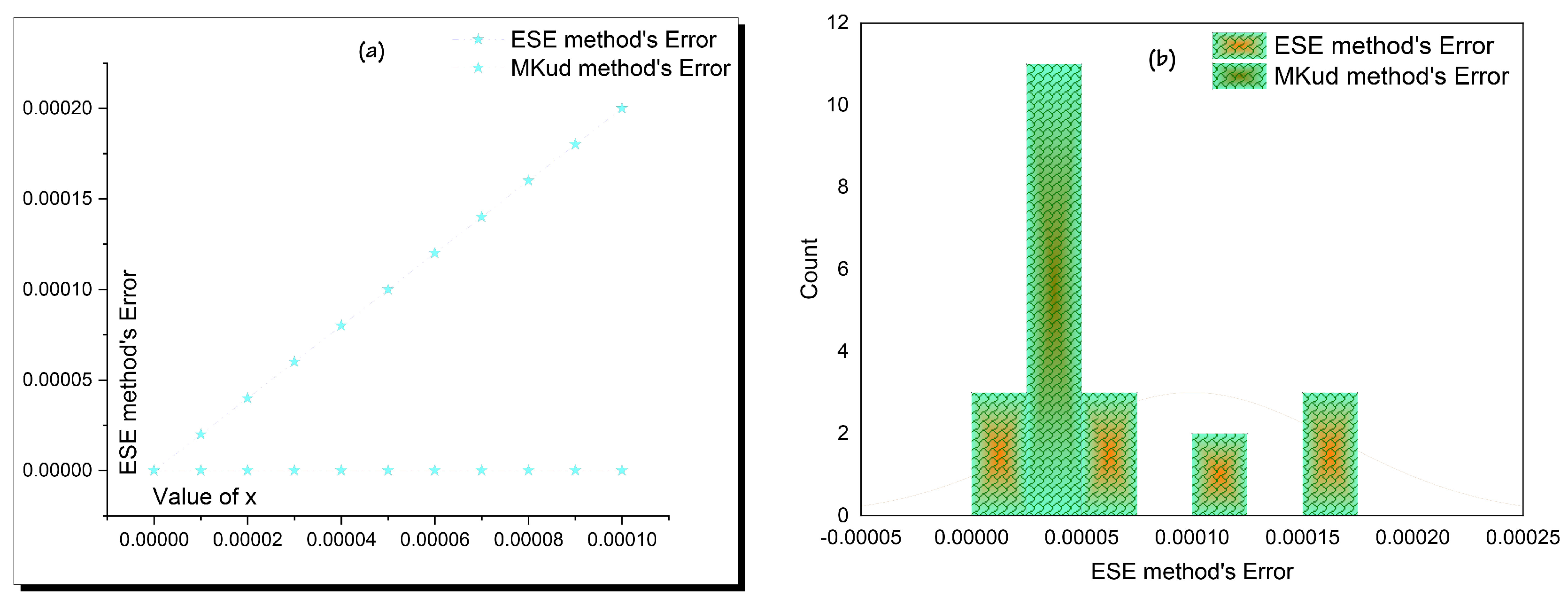
• Checking the accuracy of the obtained solutions along calculating the absolute value of error between exact and semi-analytical & numerical solutions.

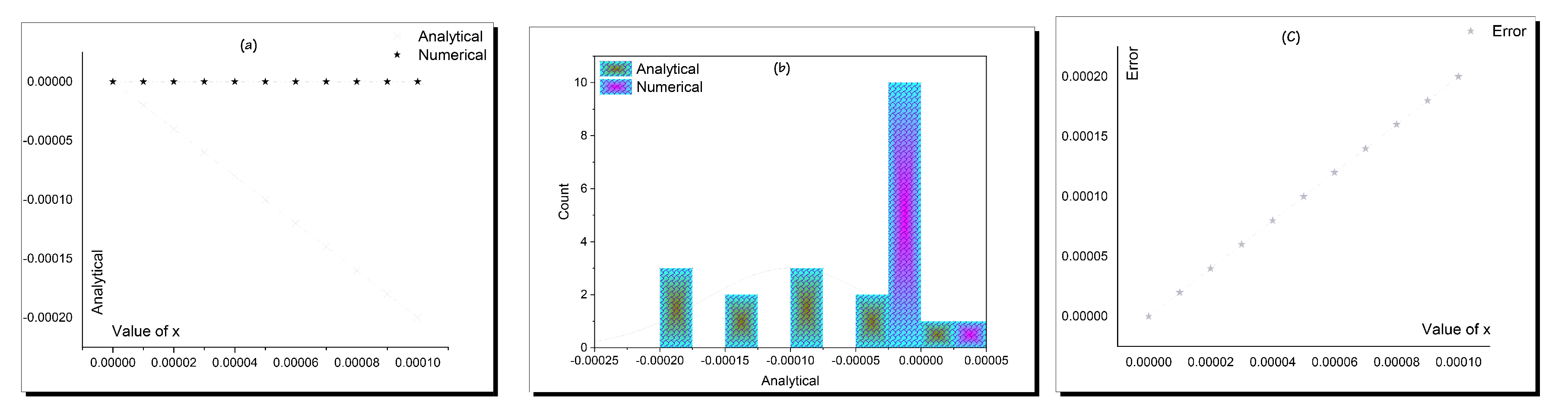
2.1. ESE Analytical vs. SBS and VI Numerical Techniques along 3-Dp-YTSF Equation

Applying the ESE scheme’s framework and its auxiliary $\left({\mathcal{C}}^{\prime }\left(\phi \right)=h_3\mathcal{C}{\left(\phi \right)}^2+h_2\mathcal{C}\left(\phi \right)+h_1\right)$, where $h_i,i=1,2,3$ are arbitrary constants to be determined later, to Equation (2), obtains the following sets of the above-mentioned parameters:

Set I

$$\begin{array}{c}\hfill \begin{array}{c}\hfill a_{-1}\to 2h_1,a_1\to 0,\lambda \to h_2^2-4h_1{h}_3+3.\end{array}\end{array}$$

Set II

$$\begin{array}{c}\hfill \begin{array}{c}\hfill a_{-1}\to 0,a_1\to -2h_3,\lambda \to h_2^2-4h_1{h}_3+3.\end{array}\end{array}$$

Therefore, the solitary solutions of (2+1)D-3-Dp-YTSF equation are constructed in the following formulas.

For $h_2=0,h_1{h}_3>0$, we get

$$\begin{array}{c}\hfill {\mathcal{Y}}_{\mathrm{I},1}(\zeta ,t)=a_0+2\sqrt{h_1{h}_3}cot\left(\sqrt{h_1{h}_3}\left(\eta +\left(3-4h_1{h}_3\right)t+\delta \right)\right),\end{array}$$

(4)

$$\begin{array}{c}\hfill {\mathcal{Y}}_{\mathrm{I},2}(\zeta ,t)=a_0+2\sqrt{h_1{h}_3}tan\left(\sqrt{h_1{h}_3}\left(\eta +\left(3-4h_1{h}_3\right)t+\delta \right)\right),\end{array}$$

(5)

$$\begin{array}{c}\hfill {\mathcal{Y}}_{\mathrm{II},1}(\zeta ,t)=a_0-2\sqrt{h_1{h}_3}tan\left(\sqrt{h_1{h}_3}\left(\eta +\left(3-4h_1{h}_3\right)t+\delta \right)\right),\end{array}$$

(6)

$$\begin{array}{c}\hfill {\mathcal{Y}}_{\mathrm{II},2}(\zeta ,t)=a_0-2\sqrt{h_1{h}_3}cot\left(\sqrt{h_1{h}_3}\left(\eta +\left(3-4h_1{h}_3\right)t+\delta \right)\right).\end{array}$$

(7)

For $h_2=0,h_1{h}_3<0$, we get

$$\begin{array}{c}\hfill {\mathcal{Y}}_{\mathrm{I},3}(\zeta ,t)=a_0-2\sqrt{-h_1{h}_3}coth\left(\sqrt{-h_1{h}_3}\left(\left(3-4h_1{h}_3\right)t+\delta \right)\mp \frac{log\left(\eta \right)}{2}\right),\end{array}$$

(8)

$$\begin{array}{c}\hfill {\mathcal{Y}}_{\mathrm{I},4}(\zeta ,t)=a_0-2\sqrt{-h_1{h}_3}tanh\left(\sqrt{-h_1{h}_3}\left(\left(3-4h_1{h}_3\right)t+\delta \right)\mp \frac{log\left(\eta \right)}{2}\right),\end{array}$$

(9)

$$\begin{array}{c}\hfill {\mathcal{Y}}_{\mathrm{II},3}(\zeta ,t)=a_0-2\sqrt{-h_1{h}_3}tanh\left(\sqrt{-h_1{h}_3}\left(\left(3-4h_1{h}_3\right)t+\delta \right)\mp \frac{log\left(\eta \right)}{2}\right),\end{array}$$

(10)

$$\begin{array}{c}\hfill {\mathcal{Y}}_{\mathrm{II},4}(\zeta ,t)=a_0-2\sqrt{-h_1{h}_3}coth\left(\sqrt{-h_1{h}_3}\left(\left(3-4h_1{h}_3\right)t+\delta \right)\mp \frac{log\left(\eta \right)}{2}\right).\end{array}$$

(11)

For $h_1=0,h_2>0$, we get

$$\begin{array}{c}\hfill {\mathcal{Y}}_{\mathrm{II},5}(\zeta ,t)=a_0+\frac{2h_2}{h_3{e}^{h_2\left(\eta +\left(h_2^2+3\right)t+\delta \right)}-1}+2h_2.\end{array}$$

(12)

For $h_1=0,h_2<0$, we get

$$\begin{array}{c}\hfill {\mathcal{Y}}_{\mathrm{II},6}(\zeta ,t)=a_0-\frac{2h_3}{h_3{e}^{h_2\left(\eta +\left(h_2^2+3\right)t+\delta \right)}+1}+2h_3.\end{array}$$

(13)

For $4h_1{h}_3>h_2^2$, we get

$$\begin{array}{c}\hfill \begin{array}{c}\hfill {\mathcal{Y}}_{\mathrm{I},5}(\zeta ,t)=a_0-\frac{4h_1{h}_3}{h_2-\sqrt{4h_1{h}_3-h_2^2}tan\left(\frac{1}{2}\sqrt{4h_1{h}_3-h_2^2}\left(\eta +\left(h_2^2-4h_1{h}_3+3\right)t+\delta \right)\right)},\end{array}\end{array}$$

(14)

$$\begin{array}{c}\hfill \begin{array}{c}\hfill {\mathcal{Y}}_{\mathrm{I},6}(\zeta ,t)=a_0-\frac{4h_1{h}_3}{h_2-\sqrt{4h_1{h}_3-h_2^2}cot\left(\frac{1}{2}\sqrt{4h_1{h}_3-h_2^2}\left(\eta +\left(h_2^2-4h_1{h}_3+3\right)t+\delta \right)\right)},\end{array}\end{array}$$

(15)

$$\begin{array}{c}\hfill \begin{array}{c}\hfill {\mathcal{Y}}_{\mathrm{II},7}(\zeta ,t)=a_0-\sqrt{4h_1{h}_3-h_2^2}tan\left(\frac{1}{2}\sqrt{4h_1{h}_3-h_2^2}\left(\eta +\left(h_2^2-4h_1{h}_3+3\right)t+\delta \right)\right)+h_2,\end{array}\end{array}$$

(16)

$$\begin{array}{c}\hfill \begin{array}{c}\hfill {\mathcal{Y}}_{\mathrm{II},8}(\zeta ,t)=a_0+\sqrt{4h_1{h}_3-h_2^2}\left(-cot\left(\frac{1}{2}\sqrt{4h_1{h}_3-h_2^2}\left(\eta +\left(h_2^2-4h_1{h}_3+3\right)t+\delta \right)\right)\right)+h_2.\end{array}\end{array}$$

(17)

Matching between Analytical and Numerical

Here, we employ two recent numerical and semi-analytical schemes to verify the accuracy of our analytical obtained solutions:

• Applying the SBS numerical technique with the following initial condition $\mathcal{Y}(x,0,0,0)=-2tanh\left(x\right)$ gets the following shown analytical and numerical solutions’ values with respect to different values of x in

  Table 1. Analytical and numerical matching through ESE and SBS schemes.

  Value of x	Analytical	Numerical	Absolute Error
  0	0	2.59953 $\times {10}^{-20}$	2.59953 $\times {10}^{-20}$
  0.00001	−0.00002	−4.94237 $\times {10}^{-14}$	0.00002
  0.00002	−0.00004	−6.43149 $\times {10}^{-14}$	0.00004
  0.00003	−0.00006	−1.08723 $\times {10}^{-13}$	0.00006
  0.00004	−0.00008	−1.13736 $\times {10}^{-13}$	0.00008
  0.00005	−0.0001	−1.48758 $\times {10}^{-13}$	0.0001
  0.00006	−0.00012	−1.44334 $\times {10}^{-13}$	0.00012
  0.00007	−0.00014	−1.69924 $\times {10}^{-13}$	0.00014
  0.00008	−0.00016	−1.56069 $\times {10}^{-13}$	0.00016
  0.00009	−0.00018	−1.72219 $\times {10}^{-13}$	0.00018
  0.0001	−0.0002	−1.49012 $\times {10}^{-13}$	−0.0002

• Applying the VI method to Equation (1), gets the following semi-analytical solutions:

  $$\begin{array}{c}\hfill {\mathcal{Y}}_{n+1}={\mathcal{Y}}_n-{\int }_0^t\left(-{\left({\mathcal{Y}}_n\right)}_{xs}+{\left({\mathcal{Y}}_n\right)}_{xxxz}+4{\left({\mathcal{Y}}_n\right)}_x{\left({\mathcal{Y}}_n\right)}_{xz}+2{\left({\mathcal{Y}}_n\right)}_{xx}{\left({\mathcal{Y}}_n\right)}_z+3{\left({\mathcal{Y}}_n\right)}_{yy}\right)ds.\end{array}$$

  (18)
  Using Equation (18)

  $$\begin{array}{c}\hfill {\mathcal{Y}}_0(\zeta ,t)=-2tanh\left(\delta \right),\end{array}$$

  (19)

  $$\begin{array}{c}\hfill {\mathcal{Y}}_1(\zeta ,t)=2tanh\left(\delta \right)\left(48t{\mathrm{sech}}^4\left(\delta \right)-14t{\mathrm{sech}}^2\left(\delta \right)-1\right),\end{array}$$

  (20)

  $$\begin{array}{c}\hfill \begin{array}{cc}\hfill {\mathcal{Y}}_2(\zeta ,t)=& 2tanh\left(\delta \right)\left(4t{\mathrm{sech}}^2\left(\delta \right)\right({\mathrm{sech}}^2\left(\delta \right)(1404t(9-28t)\hfill \\ & \times {\mathrm{sech}}^2\left(\delta \right)+48t{\mathrm{sech}}^4\left(\delta \right)(450t(3-13cosh\left(2\left(\delta \right)\right))\hfill \\ & \times {\mathrm{sech}}^4\left(\delta \right)+5683t-270)+t(1568t-2475)+24)+49t-7)-1).\hfill \end{array}\end{array}$$

  (21)
  Using same steps we can get ${\mathcal{Y}}_i,i=3,4,5,\cdots .$

2.2. Kud Analytical vs. SBS and VI Numerical Techniques along 3-Dp-YTSF Equation

Applying the MKud scheme’s framework and its auxiliary $\left({\mathcal{L}}^{\prime }\left(\phi \right)=ln\left(k\right)\left(\mathcal{L}{\left(\phi \right)}^2-\mathcal{L}\left(\phi \right)\right)\right)$, where k is arbitrary constant to be evaluated later, to Equation (2), obtains the following sets of the above-mentioned parameters:

Set I

$$\begin{array}{c}\hfill a_0=-1,a_1=2,r=2,\mu =-\frac{1}{{log}^2\left(k\right)}.\end{array}$$

Set II

$$\begin{array}{c}\hfill a_0=0,a_1=1,r=\frac{4log\left(k\right)-3}{2log\left(k\right)},\mu =-\frac{1}{4{log}^2\left(k\right)}.\end{array}$$

Set III

$$\begin{array}{c}\hfill a_0=1,a_1=-1,r=\frac{4log\left(k\right)+3}{2log\left(k\right)},\mu =-\frac{1}{4{log}^2\left(k\right)}.\end{array}$$

Therefore, the solitary solutions of 3-Dp-YTSF equation are constructed in the following formulas:

$$\begin{array}{c}\hfill \mathcal{Y}(\zeta ,t)=a_0-\frac{2log\left(k\right)}{1\pm k^{t\left({log}^2\left(k\right)+3\right)+\delta }}.\end{array}$$

(22)

Matching between Analytical, Semi-Analytical and Numerical Solutions

Here, we employ two recent numerical and semi-analytical schemes to verify the accuracy of our analytical obtained solutions:

• Applying the SBS numerical technique with the following initial condition $\mathcal{Y}(x,0,0,0)=tanh\left(\frac{x}{2}\right)$ gets the following shown analytical and numerical solutions’ values with respect to different values of x in

  Table 2. Analytical and numerical matching through MKud and SBS schemes.

  Value of x	Analytical	Numerical	Error
  0	0	2.98907 $\times {10}^{-21}$	2.98907 $\times {10}^{-21}$
  0.00001	5 $\times {10}^{-6}$	1.02496 $\times {10}^{-13}$	5$\times {10}^{-6}$
  0.00002	0.00001	1.31139 $\times {10}^{-13}$	0.00001
  0.00003	0.000015	2.19425 $\times {10}^{-13}$	0.000015
  0.00004	0.00002	2.28909 $\times {10}^{-13}$	0.00002
  0.00005	0.000025	2.98536 $\times {10}^{-13}$	0.000025
  0.00006	0.00003	2.89309 $\times {10}^{-13}$	0.00003
  0.00007	0.000035	3.40231 $\times {10}^{-13}$	0.000035
  0.00008	0.00004	3.12301 $\times {10}^{-13}$	0.00004
  0.00009	0.000045	3.44501 $\times {10}^{-13}$	0.000045
  0.0001	0.00005	2.98023 $\times {10}^{-13}$	0.00005

• Applying VI method along Equation (18) to Equation (1), obtains

  $$\begin{array}{c}\hfill {\mathcal{Y}}_0(\zeta ,t)=tanh\left(\frac{1}{2}\left(\delta \right)\right),\end{array}$$

  (23)

  $$\begin{array}{c}\hfill {\mathcal{Y}}_1(\zeta ,t)=\frac{1}{2}tanh\left(\frac{1}{2}\left(\delta \right)\right){\mathrm{sech}}^2\left(\frac{1}{2}\left(\delta \right)\right)(4t+cosh\left(\delta \right)+1),\end{array}$$

  (24)

  $$\begin{array}{c}\hfill \begin{array}{cc}\hfill {\mathcal{Y}}_2(\zeta ,t)=& \frac{1}{128}tanh\left(\frac{1}{2}\left(\delta \right)\right){\mathrm{sech}}^8\left(\frac{1}{2}\left(\delta \right)\right)(4\left(8t\left(4t^2+6t+3\right)+7\right)\hfill \\ & \times cosh\left(2\left(\delta \right)\right)+32t\left(84t^2+4t+5\right)+8(2t(7t(3-16t)+15)+7)\hfill \\ & \times cosh\left(\delta \right)+8(1-2(t-1\left)t\right)cosh\left(3\right(\delta \left)\right)+cosh\left(4\right(\delta \left)\right)+35),\hfill \end{array}\end{array}$$

  (25)
  Using same steps we can get ${\mathcal{Y}}_i,i=3,4,5,\cdots .$

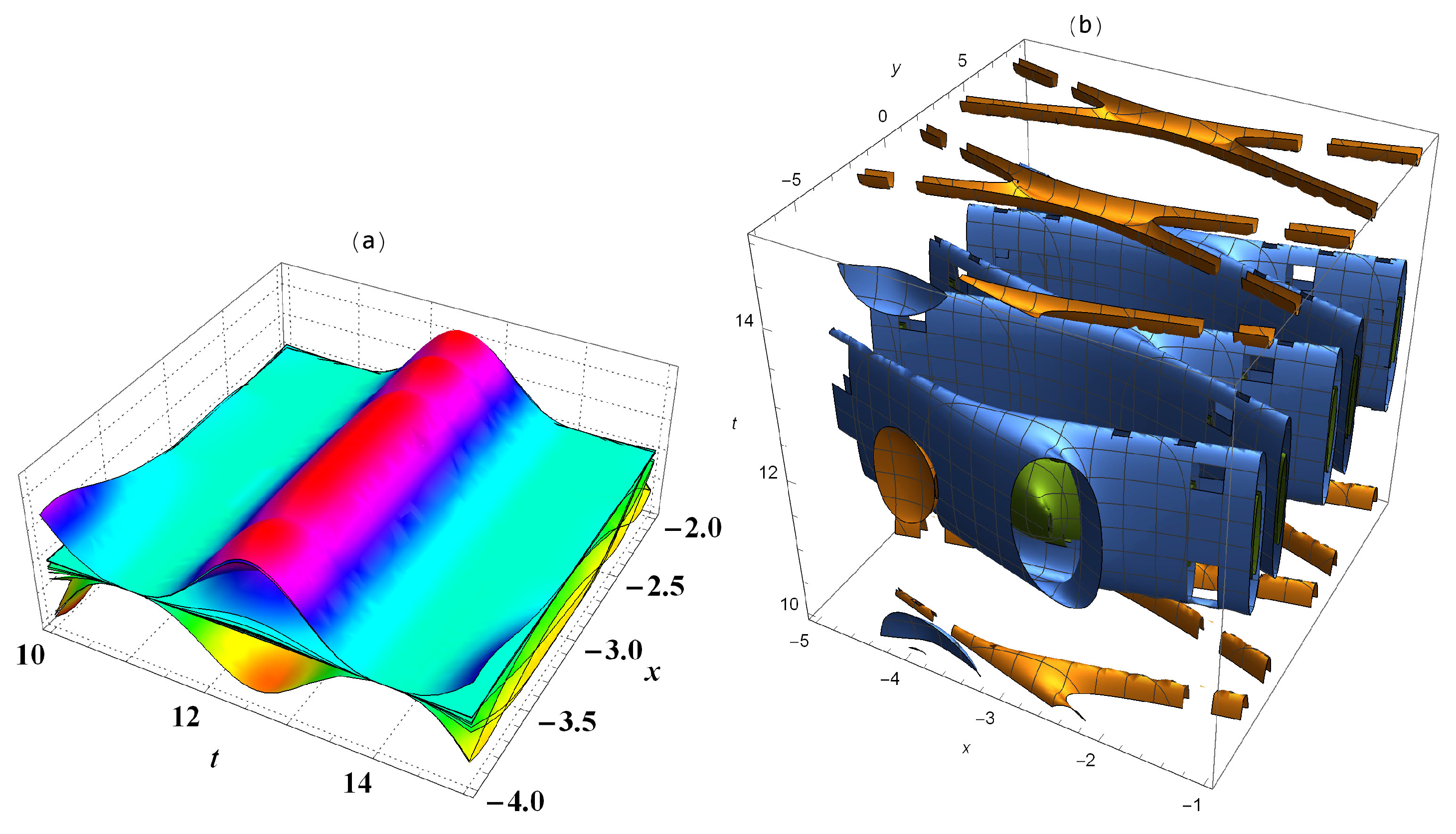
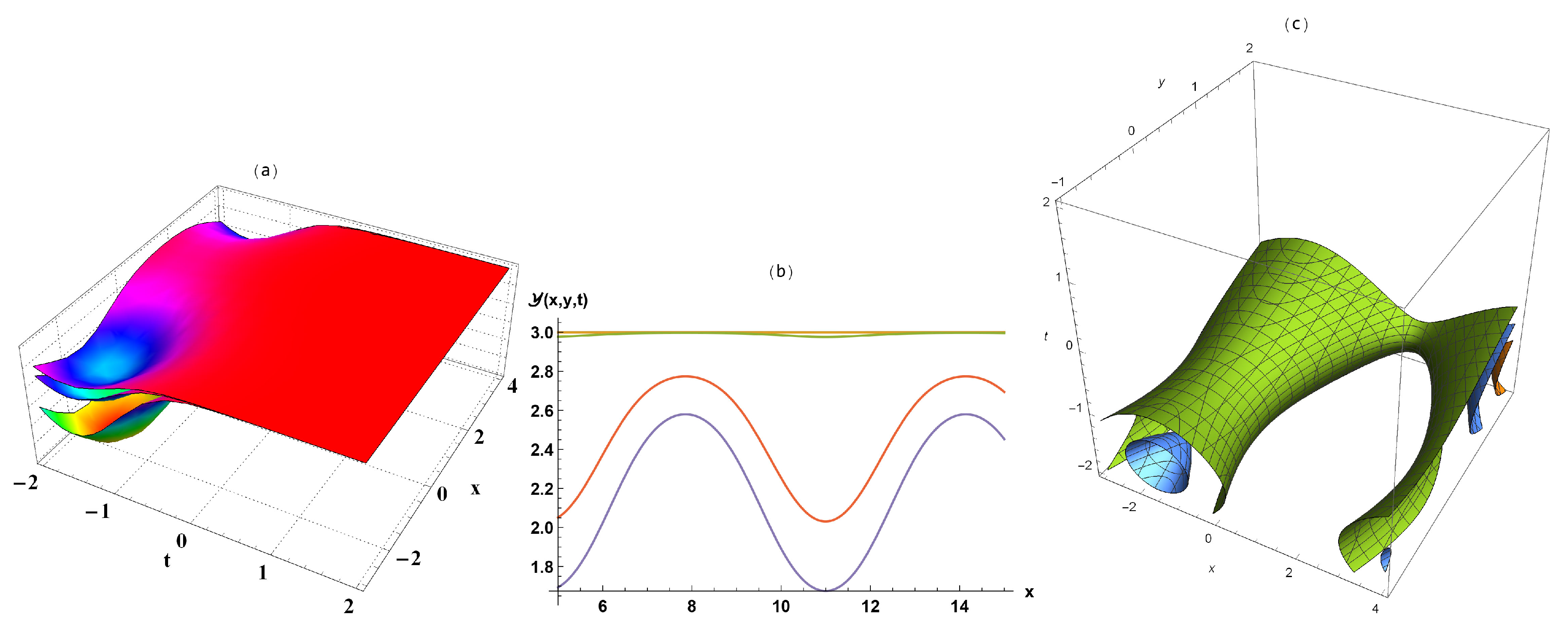
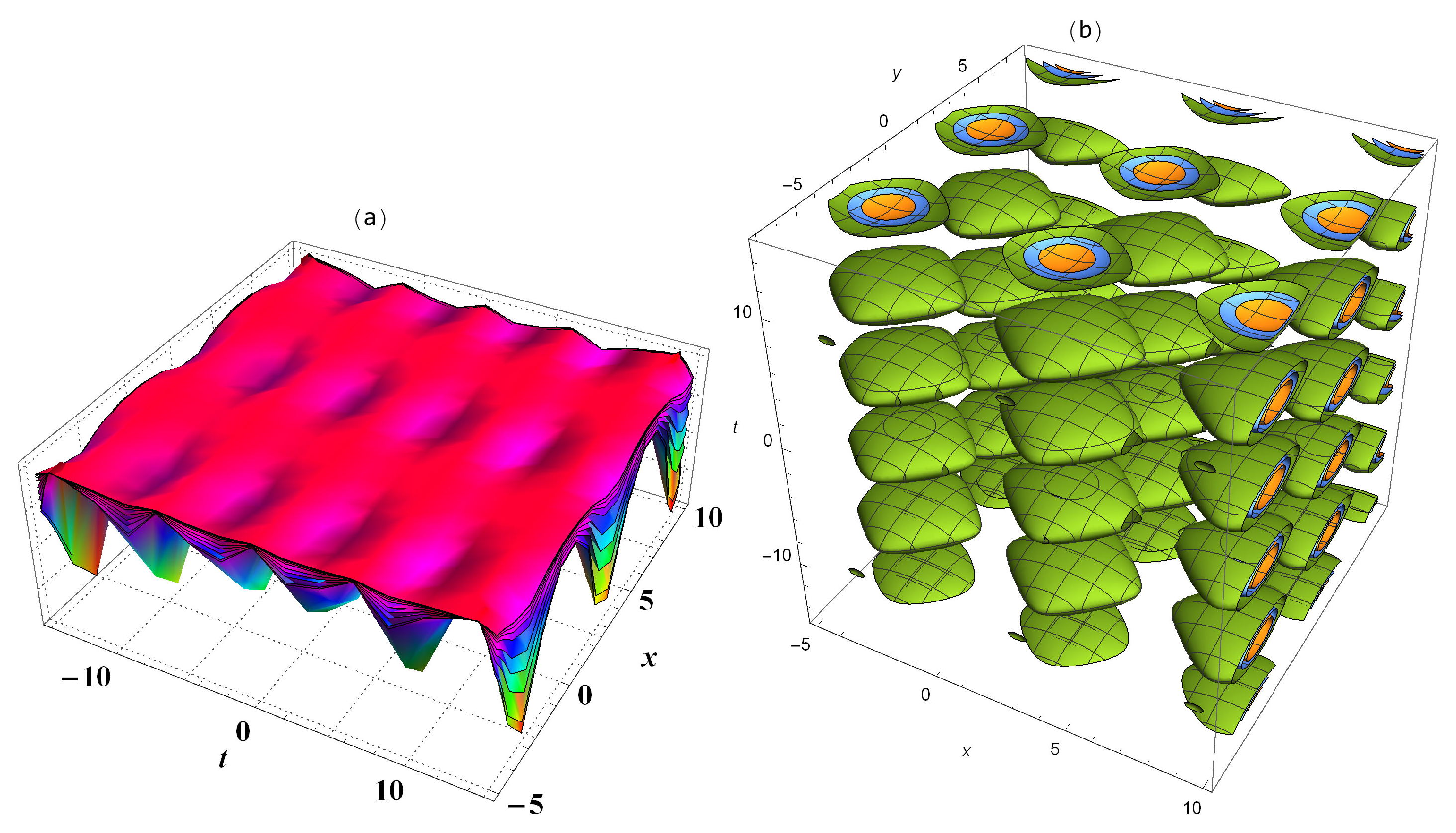
3. Results’ Interpretation

This section studies the originality and novelty of our research paper. It also shows the accuracy of the obtained analytical solutions. The ESE and MKud computational schemes were applied to the 3-Dp-YTSF equation for constructed solitary wave solutions. Many distinct wave solutions have been obtained, and some of them were demonstrated through some sketches in 2D, 3D, and contour plots to explain the dynamic behaviour of the soliton waves in weakly dispersive media. Comparing our solutions with those that were obtained in previously published papers shows our solutions are completely different from that have been evaluated in [29,30,31,32,33], but some of our solutions are matching the obtained solutions in [34] when $\left(a_0=(A_0+1),h_1{h}_3=\frac{-(3l^2+4c)}{4m},c=\lambda ,\eta =1\right)$ Equation (33) [34] are equal to Equation (9), however the authors in that paper have studied the same model with modified simplest equation method.

The SBS and VI schemes have been applied to the considered model based on the obtained computational solutions. The absolute error between the analytical and numerical solutions was calculated to show the accuracy of the solutions and used methods (Table 1 and Table 2; Figure 1 and Figure 2) while Figure 3 shows lump solitary wave solutions. While Figure 4 represents the matching between analytical and numerical solutions of Equation (1) based on Table 2. Additionally, Figure 5 demonstrates the semi–analytical solutions of Equation (1) in two and three–dimensional plots. This calculating shows the arrogance of the MKud method over the ESE method where its absolute values of error are much smaller than that have been obtained by the ESE method (Figure 6).

4. Conclusions

This research paper successfully handled the nonlinear 3-Dp-YTSF equation arising in fluid dynamics, plasma physics and weakly dispersive media. The ESE, MKud, SBS, and VI schemes were employed to find accurate novel solitary wave solutions of the considered model. Lump wave solutions have been represented in three various types of sketches. The accuracy of the MKud method has been verified over the ESE method where it is our fourth paper in series with title accuracy of the computational schemes. This series aims to determine the accuracy of all computational schemes.

References

1. Shen, B.; Chang, L.; Liu, J.; Wang, H.; Yang, Q.F.; Xiang, C.; Wang, R.N.; He, J.; Liu, T.; Xie, W.; et al. Integrated turnkey soliton microcombs. Nature 2020, 582, 365–369. [Google Scholar] [CrossRef] [PubMed]
2. Ni, G.; Wang, H.; Jiang, B.Y.; Chen, L.; Du, Y.; Sun, Z.; Goldflam, M.; Frenzel, A.; Xie, X.; Fogler, M.; et al. Soliton superlattices in twisted hexagonal boron nitride. Nat. Commun. 2019, 10, 1–6. [Google Scholar] [CrossRef] [PubMed] [Green Version]
3. Dudley, J.M.; Genty, G.; Mussot, A.; Chabchoub, A.; Dias, F. Rogue waves and analogies in optics and oceanography. Nat. Rev. Phys. 2019, 1, 675–689. [Google Scholar] [CrossRef]
4. Su, J.J.; Gao, Y.T.; Deng, G.F.; Jia, T.T. Solitary waves, breathers, and rogue waves modulated by long waves for a model of a baroclinic shear flow. Phys. Rev. E 2019, 100, 042210. [Google Scholar] [CrossRef]
5. Dematteis, G.; Grafke, T.; Onorato, M.; Vanden-Eijnden, E. Experimental evidence of hydrodynamic instantons: The universal route to rogue waves. Phys. Rev. X 2019, 9, 041057. [Google Scholar] [CrossRef] [Green Version]
6. Kannan, R.; Wang, Z. A high order spectral volume solution to the Burgers’ equation using the Hopf–Cole transformation. Int. J. Numer. Methods Fluids 2012, 69, 781–801. [Google Scholar] [CrossRef]
7. Lan, Z.Z.; Su, J.J. Solitary and rogue waves with controllable backgrounds for the non-autonomous generalized AB system. Nonlinear Dyn. 2019, 96, 2535–2546. [Google Scholar] [CrossRef]
8. Marcucci, G.; Pierangeli, D.; Conti, C. Theory of neuromorphic computing by waves: Machine learning by rogue waves, dispersive shocks, and solitons. Phys. Rev. Lett. 2020, 125, 093901. [Google Scholar] [CrossRef]
9. Kannan, R. A high order spectral volume formulation for solving equations containing higher spatial derivative terms: Formulation and analysis for third derivative spatial terms using the LDG discretization procedure. Commun. Comput. Phys. 2011, 10, 1257–1279. [Google Scholar] [CrossRef]
10. Ilhan, O.A.; Manafian, J.; Shahriari, M. Lump wave solutions and the interaction phenomenon for a variable-coefficient Kadomtsev–Petviashvili equation. Comput. Math. Appl. 2019, 78, 2429–2448. [Google Scholar] [CrossRef]
11. Kannan, R. A high order spectral volume formulation for solving equations containing higher spatial derivative terms II: Improving the third derivative spatial discretization using the LDG2 method. Commun. Comput. Phys. 2012, 12, 767–788. [Google Scholar] [CrossRef]
12. Kannan, R.; Wang, Z.J. LDG2: A variant of the LDG flux formulation for the spectral volume method. J. Sci. Comput. 2011, 46, 314–328. [Google Scholar] [CrossRef]
13. Khater, M.M.; Baleanu, D. On abundant new solutions of two fractional complex models. Adv. Differ. Equ. 2020, 2020, 1–14. [Google Scholar] [CrossRef]
14. Abdel-Aty, A.H.; Khater, M.M.; Dutta, H.; Bouslimi, J.; Omri, M. Computational solutions of the HIV-1 infection of CD4+ T-cells fractional mathematical model that causes acquired immunodeficiency syndrome (AIDS) with the effect of antiviral drug therapy. Chaos Solitons Fractals 2020, 139, 110092. [Google Scholar] [CrossRef]
15. Khater, M.M.; Attia, R.A.; Park, C.; Lu, D. On the numerical investigation of the interaction in plasma between (high & low) frequency of (Langmuir & ion-acoustic) waves. Results Phys. 2020, 18, 103317. [Google Scholar]
16. Qin, H.; Khater, M.; Attia, R.A. Inelastic Interaction and Blowup New Solutions of Nonlinear and Dispersive Long Gravity Waves. J. Funct. Spaces 2020, 2020, 5362989. [Google Scholar] [CrossRef]
17. Khater, M.M.; Ghanbari, B.; Nisar, K.S.; Kumar, D. Novel exact solutions of the fractional Bogoyavlensky–Konopelchenko equation involving the Atangana-Baleanu-Riemann derivative. Alex. Eng. J. 2020, 59, 2957–2967. [Google Scholar] [CrossRef]
18. Yue, C.; Lu, D.; Khater, M.M.; Abdel-Aty, A.H.; Alharbi, W.; Attia, R.A. On explicit wave solutions of the fractional nonlinear DSW system via the modified Khater method. Fractals 2020. [Google Scholar] [CrossRef]
19. Abdel-Aty, A.H.; Khater, M.; Attia, R.A.; Eleuch, H. Exact Traveling and Nano-Solitons Wave Solitons of the Ionic Waves Propagating along Microtubules in Living Cells. Mathematics 2020, 8, 697. [Google Scholar] [CrossRef]
20. Qin, H.; Khater, M.; Attia, R.A. Copious Closed Forms of Solutions for the Fractional Nonlinear Longitudinal Strain Wave Equation in Microstructured Solids. Math. Probl. Eng. 2020, 2020, 3498796. [Google Scholar] [CrossRef]
21. Li, J.; Attia, R.A.; Khater, M.M.; Lu, D. The new structure of analytical and semi-analytical solutions of the longitudinal plasma wave equation in a magneto-electro-elastic circular rod. Mod. Phys. Lett. B 2020, 34, 2050123. [Google Scholar] [CrossRef]
22. Khater, M.M.; Attia, R.A.; Alodhaibi, S.S.; Lu, D. Novel soliton waves of two fluid nonlinear evolutions models in the view of computational scheme. Int. J. Mod. Phys. B 2020, 34, 2050096. [Google Scholar] [CrossRef]
23. Günerhan, H.; Khodadad, F.S.; Rezazadeh, H.; Khater, M.M. Exact optical solutions of the (2+ 1) dimensions Kundu–Mukherjee–Naskar model via the new extended direct algebraic method. Mod. Phys. Lett. B 2020, 34, 2050225. [Google Scholar] [CrossRef]
24. Yue, C.; Khater, M.M.; Inc, M.; Attia, R.A.; Lu, D. Abundant analytical solutions of the fractional nonlinear (2+ 1)-dimensional BLMP equation arising in incompressible fluid. Int. J. Mod. Phys. B 2020, 34, 2050084. [Google Scholar] [CrossRef]
25. Yue, C.; Elmoasry, A.; Khater, M.; Osman, M.; Attia, R.; Lu, D.; Elazab, N.S. On complex wave structures related to the nonlinear long–short wave interaction system: Analytical and numerical techniques. AIP Adv. 2020, 10, 045212. [Google Scholar] [CrossRef] [Green Version]
26. Yue, C.; Khater, M.M.; Attia, R.A.; Lu, D. Computational simulations of the couple Boiti–Leon–Pempinelli (BLP) system and the (3+ 1)-dimensional Kadomtsev–Petviashvili (KP) equation. AIP Adv. 2020, 10, 045216. [Google Scholar] [CrossRef] [Green Version]
27. Khater, M.M.; Attia, R.A.; Lu, D. Computational and numerical simulations for the nonlinear fractional Kolmogorov–Petrovskii–Piskunov (FKPP) equation. Phys. Scr. 2020, 95, 055213. [Google Scholar] [CrossRef]
28. Khater, M.M.; Alzaidi, J.; Attia, R.A.; Lu, D. Analytical and numerical solutions for the current and voltage model on an electrical transmission line with time and distance. Phys. Scr. 2020, 95, 055206. [Google Scholar] [CrossRef]
29. Dong, M.J.; Tian, S.F.; Wang, X.B.; Zhang, T.T. Lump-type solutions and interaction solutions in the (3+ 1)-dimensional potential Yu–Toda–Sasa–Fukuyama equation. Anal. Math. Phys. 2019, 9, 1511–1523. [Google Scholar] [CrossRef]
30. Hu, Y.; Chen, H.; Dai, Z. New kink multi-soliton solutions for the (3+ 1)-dimensional potential-Yu–Toda–Sasa– Fukuyama equation. Appl. Math. Comput. 2014, 234, 548–556. [Google Scholar] [CrossRef]
31. Zhang, S.; Zhang, H.Q. A transformed rational function method for (3+ 1)-dimensional potential Yu–Toda–Sasa–Fukuyama equation. Pramana 2011, 76, 561–571. [Google Scholar] [CrossRef]
32. Liu, W. Rogue waves of the (3+ 1)-dimensional potential Yu–Toda–Sasa–Fukuyama equation. Rom. Rep. Phys. 2017, 69, 16. [Google Scholar]
33. Roshid, H.O. Lump solutions to a (3+ 1)-dimensional potential-Yu–Toda–Sasa–Fukuyama (YTSF) like equation. Int. J. Appl. Comput. Math. 2017, 3, 1455–1461. [Google Scholar] [CrossRef]
34. Zayed, E.; Arnous, A. Exact solutions of the nonlinear ZK-MEW and the potential YTSF equations using the modified simple equation method. AIP Conf. Proc. 2012, 1479, 2044–2048. [Google Scholar]
Figure 1. Analytical, numerical represented in two dimensional (a), column plot (b), while absolute error for Equation (1) is represented in two dimensional (c) with respect to Table 1.
Symmetry 12 02081 g001
Figure 2. Semi-analytical solutions of Equation (2) in three-dimensional (a) and contour plots (b).
Symmetry 12 02081 g002
Figure 3. Solitary wave solutions Equation (22) in three (a), two (b), and contour plots (c).
Symmetry 12 02081 g003
Figure 4. Analytical, numerical represented in two dimensional (a), column plot (b), while absolute error for Equation (1) is represented in two dimensional (c) with respect to Table 2.
Symmetry 12 02081 g004
Figure 5. Semi-analytical solutions of Equation (1) in three-dimensional (a) and contour plots (b).
Symmetry 12 02081 g005
Figure 6. Absolute error along ESE, MKud analytical schemes and TQBS numerical scheme in two dimensional (a) and column plots (b).
Symmetry 12 02081 g006