Numerical Solution of Nonlinear Fredholm and Volterra Integrals by Newton–Kantorovich and Haar Wavelets Methods

Abstract

The current study proposes a numerical method which solves nonlinear Fredholm and Volterra integral of the second kind using a combination of a Newton–Kantorovich and Haar wavelet. Error analysis for the Holder classes was established to ensure convergence of the Haar wavelets. Numerical examples will illustrate the accuracy and simplicity of Newton–Kantorovich and Haar wavelets. Numerical results of the current method were then compared with previous well-established methods.

1. Introduction

The application of integral equations can be found in various fields which include mathematics, physics and engineering. The process of solving the integral equations analytically is very complicated and for application purposes, it will be sufficient to solve the latter numerically. Previously, many methods have been established to find numerical solutions for integral equations. These methods include the polynomial approximation [1,2], linear multistep methods [3], modified homotopy perturbation [4], wavelets [5,6,7,8,9], triangular functions [10] and Newton–Kantorovich method [11,12,13,14]. A few of the mentioned methods are applicable to merely linear integrals whereas the latter are capable of approximating nonlinear integral equations. Finding the numerical solutions for integral equations are often a complicated process and requires a large number of arithmetic computations. Therefore, a simple and efficient technique that can solve both linear and nonlinear integral equations is needed.

This research aims to present a numerical method which approximates nonlinear Fredholm integrals

$$x\left(t\right)=f\left(t\right)+{\int }_0^{1}K(t,s)\sum _{l=0}^m{f}_l\left(s\right)x^l\left(s\right)ds,m>1,$$

(1)

and nonlinear Volterra integral

$$x\left(t\right)=f\left(t\right)+{\int }_0^{t}K(t,s)\sum _{l=0}^m{f}_l\left(s\right)x^l\left(s\right)ds,m>1,$$

(2)

both of the second kind. The functions $f,f_l\in L^2[0,1],l=0,1,\dots ,m$, $K(t,s)\in L^2[0,1]\times [0,1]$ are given functions whereas, $x\left(t\right)$ is the unknown function with m as a positive integer. This article is organized as follows: following the introduction section, Section 2 and Section 3 provides the preliminaries and approximation of the functions by Haar wavelets; numerical solutions for both nonlinear Fredholm and Volterra integrals are then constructed in Section 4 and Section 5 respectively; error analysis for Haar wavelets which is derived in Section 6 satisfies the conditions in Holder space; the numerical results are reported in Section 7; while the conclusion is elaborated in Section 8.

2. Preliminaries

Theorem 1.

The solution of system

$$x_n\left(t_p\right)=\sum _{n=1}^{2N}{c}_n{h}_n\left(t_p\right),p=1,2,\dots ,2N,$$

is established as below:

$$\begin{array}{cc}\hfill & c_1=\frac{1}{2N}\sum _{j=1}^{2N}x\left(t_j\right)\hfill \\ \hfill & c_i=\frac{1}{{\rho }_i}\left(\sum _{p={\alpha }_i}^{{\beta }_i}x\left(t_p\right)-\sum _{p={\beta }_i+1}^{{\gamma }_i}x\left(t_p\right)\right),i=2,3,\dots ,2N,\hfill \end{array}$$

(3)

where

$$\begin{array}{cc}\hfill & {\alpha }_i={\rho }_i({\sigma }_i-1)+1,\hfill \\ \hfill & {\beta }_i={\rho }_i({\sigma }_i-1)+\frac{{\rho }_i}{2},\hfill \\ \hfill & {\gamma }_i={\rho }_i{\sigma }_i,\hfill \\ \hfill & {\rho }_i=\frac{2N}{{\tau }_i},\hfill \\ \hfill & {\sigma }_i=i-{\tau }_i,\hfill \\ \hfill & {\tau }_i=2^{\lfloor lo{g}_2(i-1)\rfloor }.\hfill \end{array}$$

(4)

See [6,15].

Corollary 1.

The solution of the system

$$K_N(t,s_p)=\sum _{n=1}^{2N}{c}_n\left(t\right)h_n\left(s_p\right),p=1,2,\dots ,2N,$$

is defined below:

$$\begin{array}{cc}\hfill & c_1\left(t\right)=\frac{1}{2N}\sum _{j=1}^{2N}K(t,s_j)\hfill \\ \hfill & c_i\left(t\right)=\frac{1}{{\rho }_i}\left(\sum _{p={\alpha }_i}^{{\beta }_i}K(t,s_p)-\sum _{p={\beta }_i+1}^{{\gamma }_i}K(t,s_p)\right),i=2,3,\dots ,2N,\hfill \end{array}$$

(5)

where ${\tau }_i,{\sigma }_i,{\beta }_i,{\alpha }_i$ and ${\rho }_i$ are illustrated in Theorem 1. See [8].

Definition 1.

The set of all continuous functions on $[0,1]$, which satisfies the inequality

$$\left|f\left(t\right)-f\left(y\right)\right|\le L{\left|t-y\right|}^s,L>0,\forall t,y\in [0,1].$$

is called a Holder space of order s and denoted by $H^s[0,1]$ whereas, the norm is given by

$${∥f∥}_{H^s[0,1]}={∥f∥}_{C[0,1]}+\underset{t\ne y}{sup}\frac{\left|f\left(t\right)-f\left(y\right)\right|}{{\left|t-y\right|}^s},$$

for all $t,y\in [0,1]$.

3. Establishing Haar Wavelets

Haar wavelets are selected to solve the Equations (1) and (2) due to fact that they are the most simple orthonormal wavelets with compact support. The Haar wavelets are defined on the interval $[0,1)$ by

$$H\left(x\right)=\left\{\begin{array}{cc}\hfill 1,& x\in [0,\frac{1}{2})\hfill \\ \hfill -1,& x\in [\frac{1}{2},1)\hfill \\ \hfill 0,& elsewhere,\hfill \end{array}\right.$$

where,

$$h_n\left(x\right)=2^{\frac{j}{2}}H(2^{j}x-k),n=2^j+k,j=0,1,2,\dots ,k=0,1,\dots ,2^j-1$$

which forms an orthonormal system:

$${\int }_0^1{h}_n\left(x\right)h_{\ell }\left(x\right)dx=\left\{\begin{array}{cc}\hfill 1,& n=\ell =2^j+k\hfill \\ \hfill 0,& n\ne \ell .\hfill \end{array}\right.$$

Any square integrable function, $x\left(t\right)$ over the interval $(0,1)$ can be approximated using Haar wavelets as follows:

$$x\left(t\right)=\sum _{n=1}^{\infty }{c}_n{h}_n\left(t\right).$$

(6)

In practice, the series (6) is truncated as

$$x\left(t\right)\simeq x_N\left(t\right)=\sum _{n=1}^{2N}{c}_n{h}_n\left(t\right),$$

(7)

where $N=2^{\beta },\beta =0,1,2,\dots ,$ and $c_n$ are the unknown coefficients. To evaluate the coefficients $c_n,$ we need to consider these collocation points

$$t_p=\frac{p-0.5}{2N},p=1,2,\dots ,2N.$$

(8)

Next, by substituting the collocation points (8) into (6), we obtain the following $2N\times 2N$ linear system of equations

$$x_n\left(t_p\right)=\sum _{n=1}^{2N}{c}_n{h}_n\left(t_p\right),p=1,2,\dots ,2N,$$

(9)

which could be written in the matrix form

$$x_n\left(t_p\right)=H^{T}C,$$

where H is an $2N\times 2N$ with $h_{ij}=h_i\left(t_j\right)$ and unknown coefficients, $C={[c_1,c_2,\dots ,c_n]}^T$. The H is an asymmetric Haar with only element $1,-1$ or 0. Here we do not need to solve the above system which is computationally expensive for large values of N, thus Theorem 1 gives us a simple formula to calculate the coefficients $c_n$.

Let $K(t,s)$ be a square integrable function with variables t and s where the function $K(t,s)$ is approximated using the Haar wavelet basis as

$$K(t,s)\simeq K_N(t,s)=\sum _{n=1}^{2N}{c}_n\left(t\right)h_n\left(s\right).$$

(10)

Substituting (8) into (10) yields the following system of $2N\times 2N$ linear equations

$$K_N(t,s_p)=\sum _{n=1}^{2N}{c}_n\left(t\right)h_n\left(s_p\right),p=1,2,\dots ,2N,$$

(11)

where the corollary 1 above denotes an algorithm for finding the unknown coefficients $c_i\left(t\right),i=1,2,\dots ,2N$.

4. Nonlinear Fredholm Integral of the Second Kind

This section provides the derivation for solving nonlinear Fredholm integral of the second kind. Firstly consider the following nonlinear Fredholm integral of the second kind

$$x\left(t\right)=f\left(t\right)+{\int }_0^{1}K(t,s)\sum _{l=0}^m{f}_l\left(s\right)x^l\left(s\right)ds,m>1,$$

(12)

which can be rewritten in the operator form

$$P\left(x\right)=x\left(t\right)-{\int }_0^{1}K(t,s)\sum _{l=0}^m{f}_l\left(s\right)x^l\left(s\right)ds-f\left(t\right).$$

The initial iteration of Newton–Kantorovich method is described as

$$P^{\prime }\left(x_0\right)(x-x_0)+P\left(x_0\right)=0,$$

(13)

where $x_0=x_0\left(t\right)$ is the initial guess and is a continuously differentiable function in the interval $[0,1]$. $P^{\prime }\left(x_0\right)$ is the derivative of $P\left(x\right)$ at the point $x_0$. By the method of iteration, we obtain a sequence of linear integral equations as follows:

$$\begin{array}{cc}\hfill & \Delta x_i\left(t\right)-{\int }_0^{1}K(t,s)\Delta x_i\left(s\right)\sum _{l=0}^{m}l{f}_l\left(s\right)x_0^{l-1}\left(s\right)ds\hfill \\ \hfill & =f\left(t\right)-x_{i-1}\left(t\right)+{\int }_0^{1}K(t,s)\sum _{l=0}^m{f}_l\left(s\right)x_{i-1}^l\left(s\right)ds,\hfill \end{array}$$

(14)

where $\Delta x_i\left(t\right)=x_i\left(t\right)-x_{i-1}\left(t\right),i=1,2,3,\dots$.

Therefore, the nonlinear Fredholm integral Equation (12) is reduced to a sequence of linear integral Equations (14). The Newton–Kantorovich method constructs a sequence of functions that will converge to the solution (13). The Newton–Kantorovich theorem was first introduced by Leonid Kantorovich in 1948 since then, many studies and applications have been done in this area (see [13,14,16,17,18,19]).

Next, substitute $i=1$ in the linear Fredholm integral (14) to obtain

$$\Delta x_1\left(t\right)+{\int }_0^1{K}_1(t,s)\Delta x_1\left(s\right)ds=f\left(t\right)-x_0\left(t\right)+{\int }_0^{1}K(t,s)\sum _{l=0}^m{f}_l\left(s\right)x_0^l\left(s\right)ds,$$

(15)

where $K_1(t,s)=K(t,s){\displaystyle \sum _{l=0}^m}l{f}_l\left(s\right)x_0^{l-1}\left(s\right).$ Subsequently, the functions $\Delta x_1\left(t\right)$ and $K_1(t,s)\Delta x_1\left(s\right)$ are approximated as

$$\Delta x_1\left(t\right)\simeq \sum _{n=1}^{2N}{c}_n{h}_n\left(t\right),$$

(16)

$$K_1(t,s)\Delta x_1\left(s\right)\simeq \sum _{n=1}^{2N}{d}_n\left(t\right)h_n\left(s\right),$$

(17)

where

$$d_1\left(t\right)=\frac{1}{2N}\sum _{j=1}^{2N}{K}_1(t,s_j)\Delta x_1\left(s_j\right)$$

and

$$d_i\left(t\right)=\frac{1}{{\rho }_i}\left(\sum _{p={\alpha }_i}^{{\beta }_i}{K}_1(t,s_p)\Delta x_1\left(s_p\right)-\sum _{p={\beta }_i+1}^{{\gamma }_i}{K}_1(t,s_p)\Delta x_1\left(s_p\right)\right),i=2,3,\dots ,2N.$$

The functions $d_i\left(t\right),i=1,2,\dots ,2N$ are derived using Equation (5), then Equations (16) and (17) are substituted into (15) to get:

$$\sum _{n=1}^{2N}{c}_n{h}_n\left(t\right)+\sum _{n=1}^{2N}{d}_n\left(t\right){\int }_0^1{h}_n\left(s\right)ds=f\left(t\right)-x_0\left(t\right)+{\int }_0^{1}K(t,s)\sum _{l=0}^m{f}_l\left(s\right)x_0^l\left(s\right)ds.$$

(18)

Since ${\int }_0^1{h}_n\left(s\right)ds=0$ for all $n=2,3,\dots ,2N$ and ${\int }_0^1{h}_1\left(s\right)ds=1$ then Equation (18) reduce to

$$\sum _{n=1}^{2N}{c}_n{h}_n\left(t\right)+d_1\left(t\right)=f\left(t\right)-x_0\left(t\right)+{\int }_0^{1}K(t,s)\sum _{l=0}^m{f}_l\left(s\right)x_0^l\left(s\right)ds.$$

(19)

Only the left side of Equation (18) is expanded by Haar wavelets, because of the unknown function $\Delta x_1\left(t\right)$, whereas, the right hand side are given functions including $x_0\left(t\right)$. Equation (19) is then utilized by the collocation points (8) to attain $2N\times 2N$ linear system of equations

$$\sum _{n=1}^{2N}{c}_n{h}_n\left(t_p\right)+d_1\left(t_p\right)=f\left(t_p\right)-x_0\left(t_p\right)+{\int }_0^{1}K(t_p,s)\sum _{l=0}^m{f}_l\left(s\right)x_0^l\left(s\right)ds,$$

(20)

where $p=1,2,\dots ,2N$. Solving the linear algebraic system (20), we get $x_1\left(t\right),$ given that $x_1\left(t\right)=\Delta x_1\left(t\right)+x_0\left(t\right).$ By repeating this procedure (20), we obtain the values $x_2\left(t\right),x_3\left(t\right),\dots$ for a selected $i\in 1,2,3,\dots ,$ in order to provide better approximation of $x\left(t\right)$.

In general, the sequence of $x_i\left(t\right)$ can be evaluated by solving the following equation

$$\Delta x_i\left(t\right)+{\int }_0^1{K}_1(t,s)\Delta x_i\left(s\right)ds=f\left(t\right)-x_{i-1}\left(t\right)+{\int }_0^{1}K(t,s)\sum _{l=0}^m{f}_l\left(s\right)x_{i-1}^l\left(s\right)ds,$$

where $\Delta x_i\left(t\right)=x_i\left(t\right)-x_{i-1}\left(t\right)i=1,2,3,\dots ,$ in order to achieve better approximation of $x\left(t\right)$.

After a few iterations, the approximated solution $x_i\left(t\right)$ stacks at a certain level of iteration and is not gaining better results. Therefore, we need to increase the number of bases N for the Haar wavelets as to improve the approximated solution of $x_i\left(t\right)$. The consequence of increasing the number of bases N increases the computational effort. Fortunately, the problem can be avoided. Due to the Haar wavelets figure (step functions), one’s could take the average of the approximated solution $x_i\left(t\right)$ below:

$$S_1\left(t\right)=\frac{x_i\left(t\right)+x_i(t+\frac{1}{2N})}{2},$$

and allign back the approximated solution as

$$S_{j+1}\left(t\right)=\frac{S_j\left(t\right)+S_j(t-\frac{1}{2N})}{2}j=1,2,3,\dots .$$

(21)

The Equation (21) will perform a better approximation solution than $x_i\left(t\right)$ without any increase in the number of bases N for the Haar wavelets. Next, we proceed with the nonlinear Volterra integral of the second kind.

5. Nonlinear Volterra Integral of the Second Kind

The general nonlinear Volterra integral of the second kind is formulated as.

$$x\left(t\right)=f\left(t\right)+{\int }_0^{t}K(t,s)\sum _{l=0}^m{f}_l\left(s\right)x^l\left(s\right)ds,m>1.$$

Using similar techniques, the Fredholm integral is reduced via the Newton–Kantorovich method produces a sequence of linear Volterra integral equations

$$\begin{array}{cc}\hfill & \Delta x_i\left(t\right)-{\int }_0^{t}K(t,s)\Delta x_i\left(s\right)\sum _{l=0}^{m}l{f}_l\left(s\right)x_0^{l-1}\left(s\right)ds\hfill \\ \hfill & =f\left(t\right)-x_{i-1}\left(t\right)+{\int }_0^{t}K(t,s)\sum _{l=0}^m{f}_l\left(s\right)x_{i-1}^l\left(s\right)ds,\hfill \end{array}$$

(22)

where $\Delta x_i\left(t\right)=x_i\left(t\right)-x_{i-1}\left(t\right)$. Next, substitute $i=1$ in the Equation (22) to obtain

$$\Delta x_1\left(t\right)+{\int }_0^t{K}_1(t,s)\Delta x_1\left(s\right)ds=f\left(t\right)-x_0\left(t\right)+{\int }_0^{t}K(t,s)\sum _{l=0}^m{f}_l\left(s\right)x_0^l\left(s\right)ds,$$

(23)

where $K_1(t,s)=K(t,s){\displaystyle \sum _{l=0}^m}l{f}_l\left(s\right)x_0^{l-1}\left(s\right).$ By approximating the functions $\Delta x_1\left(t\right)$ and $K_1(t,s)\Delta x_1\left(s\right)$ using the Equations (16) and (17) and substituting it into Equation (23) yields

$$\sum _{n=1}^{2N}{c}_n{h}_n\left(t\right)+\sum _{n=1}^{2N}{d}_n\left(t\right){\int }_0^t{h}_n\left(s\right)ds=f\left(t\right)-x_0\left(t\right)+{\int }_0^{t}K(t,s)\sum _{l=0}^m{f}_l\left(s\right)x_0^l\left(s\right)ds.$$

(24)

Similarly to the Fredholm integral, we only expand the left side of the Equation (24) by the Haar wavelets. Then, we substitute Equation (24) using the collocation points from (8) and get the following $2N\times 2N$ linear system of equation:

$$\sum _{n=1}^{2N}{c}_n{h}_n\left(t_p\right)+\sum _{n=1}^{2N}{d}_n\left(t_p\right){\int }_0^{t_p}{h}_n\left(s\right)ds=f\left(t_p\right)-x_0\left(t_p\right)+{\int }_0^{t_p}K(t_p,s)\sum _{l=0}^m{f}_l\left(s\right)x_0^l\left(s\right)ds.$$

By solving this linear system, we obtain $x_1\left(t\right)$ where, $x_1\left(t\right)=\Delta x_1\left(t\right)+x_0\left(t\right).$ For a better approximation of $x\left(t\right),$ this process is repeated to find $x_2\left(t\right),x_3\left(t\right),\dots$ until a sufficient solution for $x_i\left(t\right)$ is obtained. Finally, to achieve a better approximation than $x_i\left(t\right)$ without increasing the number of Haar wavelet bases N as mentioned in the previous section, the sufficient solution $x_i\left(t\right)$ is substituted into Equation (21).

6. Error Analysis

Let $x_i\left(t\right)\in L_2[0,1]$ be sequence of functions which satisfy

$$\begin{array}{cc}\hfill & \Delta x_i\left(t\right)-{\int }_0^{1}K(t,s)\Delta x_i\left(s\right)\sum _{l=0}^{m}l{f}_l\left(s\right)x_0^{l-1}\left(s\right)ds\hfill \\ \hfill & =f\left(t\right)-x_{i-1}\left(t\right)+{\int }_0^{1}K(t,s)\sum _{l=0}^m{f}_l\left(s\right)x_{i-1}^l\left(s\right)ds,\hfill \end{array}$$

(25)

where $\Delta x_i\left(t\right)=x_i\left(t\right)-x_{i-1}\left(t\right),i=1,2,3,\dots ,$ and the Haar wavelet expansion of $\Delta x_i$ be

$$\Delta x_i\left(t\right)=\sum _{n=0}^{\infty }{c}_n{h}_n\left(t\right).$$

Theorem 2.

If the sequence $x_i\left(t\right)$ satisfy the Lipschitz condition with $0<s<1$ then

$${∥\sum _{n=M}^{\infty }{c}_n{h}_n\left(t\right)∥}_{L_2[0,1]}\le \frac{L^2}{2(4^s-1)M^{2s}}.$$

Proof. 

Let $M=2^{\beta +1},\beta =0,1,2,\dots ,$ then by taking the error in $L^2[0,1]$ norm,

$${∥\sum _{n=2^{\beta +1}}^{\infty }{c}_n{h}_n\left(t\right)∥}_{L_2[0,1]}^2=\sum _{n=2^{\beta +1}}^{\infty }\sum _{n^{\prime }=2^{{\beta }^{\prime }+1}}^{\infty }{c}_n{c}_{n^{\prime }}{\int }_0^1{h}_n\left(t\right)h_{n^{\prime }}\left(t\right)dt=\sum _{n=2^{\beta +1}}^{\infty }{c}_n^2,$$

where

$$c_n=〈\Delta x_i,h_n〉={\int }_0^1\Delta x_i\left(t\right)h_n\left(t\right)dt.$$

From definition of the Haar wavelets:

$$h_n\left(t\right)=2^{\frac{j}{2}}H(2^{j}t-k),k=0,1,...2^j-1,j=0,1,...,$$

$$H(2^{j}t-k)=\left\{\begin{array}{c}1fort\in \left[k{2}^{-j}\right.,\left.\left(k+\frac{1}{2}\right)2^{-j}\right),\hfill \\ -1fort\in \left[\left(k+\frac{1}{2}\right)2^{-j}\right.,\left.\left(k+1\right)2^{-j}\right),\hfill \\ 0elsewhere,\hfill \end{array}\right.$$

we obtain

$$\begin{array}{cc}\hfill c_n=〈\Delta x_i,h_n〉=& {\int }_0^1{2}^{\frac{j}{2}}\Delta x_i\left(t\right)H(2^{j}t-k)dt,\hfill \\ \hfill =& 2^{\frac{j}{2}}\left({\int }_{k{2}^{-j}}^{(k+\frac{1}{2})2^{-j}}\Delta x_i\left(t\right)dt-{\int }_{(k+\frac{1}{2})2^{-j}}^{(k+1)2^{-j}}\Delta x_i\left(t\right)dt\right).\hfill \end{array}$$

By changing the limit of integration in the above equation from

$$\left(k+\frac{1}{2}\right)2^{-j}\le t<(k+1)2^{-j},$$

to

$$k{2}^{-j}\le t-2^{-j-1}<\left(k+\frac{1}{2}\right)2^{-j},$$

yields

$$\begin{array}{cc}\hfill c_n=& 2^{\frac{j}{2}}\left({\int }_{k{2}^{-j}}^{(k+\frac{1}{2})2^{-j}}\Delta x_i\left(t\right)dt-{\int }_{k{2}^{-j}}^{(k+\frac{1}{2})2^{-j}}\Delta x_i(x+2^{-j-1})dt\right),\hfill \\ \hfill =& 2^{\frac{j}{2}}{\int }_{k{2}^{-j}}^{(k+\frac{1}{2})2^{-j}}\left(\Delta x_i\left(t\right)-\Delta x_i(t+2^{-j-1})\right)dt.\hfill \end{array}$$

Taking into account that the sequence of function $x_i\left(t\right)$

$$\left|x_i(t+h)-x_i\left(t\right)\right|\le L{\left|h\right|}^s,L>0\forall t,h\in [0,1].$$

The latter allow us to estimate the coefficients $c_n$ as follows

$$\begin{array}{cc}\hfill \left|c_n\right|\le & 2^{\frac{j}{2}}{\int }_{k{2}^{-j}}^{(k+\frac{1}{2})2^{-j}}\left|\Delta x_i\left(t\right)-\Delta x_i(t+2^{-j-1})\right|dt,\hfill \\ \hfill \le & 2^{\frac{j+2}{2}}L{2}^{s(-j-1)}{\int }_{k{2}^{-j}}^{(k+\frac{1}{2})2^{-j}}dt=L{2}^{s(-j-1)-\frac{j}{2}}.\hfill \end{array}$$

Hence, we have arrived to the final estimation for the coefficients

$$c_n^2\le L^2{2}^{-2s(j+1)-j}.$$

Therefore,

$$\begin{array}{cc}\hfill {∥\sum _{n=M}^{\infty }{c}_n{h}_n\left(t\right)∥}^2=& \sum _{n=2^{\beta +1}}^{\infty }{c}_n^2\le \sum _{n=2^{\beta +1}}^{\infty }{L}^2{2}^{-2s(j+1)-j},\hfill \\ \hfill =& \frac{2L^2}{4^{s+1}}\sum _{j=\beta +1}^{\infty }\sum _{n=2^j}^{2^{j+1}-1}{2}^{-2sj-j}=\frac{2L^2}{4^{s+1}}\sum _{j=\beta +1}^{\infty }{2}^{-2sj},\hfill \\ \hfill =& \frac{L^2}{2\left(4^s-1\right)M^{2s}}.\hfill \end{array}$$

Finally

$${∥\sum _{n=M}^{\infty }{c}_n{h}_n\left(t\right)∥}_{{}_{L_2[0,1]}}^2\le \frac{L^2}{2\left(4^s-1\right)M^{2s}}.$$

This completes the proof of the Theorem 2. □

We note that Ahmedov et al. [20] have shown that the error in $L^2[0,1]$ norm is given by

$${∥f-f_N∥}_{L_2[0,1]}\le \frac{L^2}{4(4^s-1)N^{2s}},$$

if $f\left(t\right)\in H^s[0,1],0<s<1$. This ensures that the Haar wavelet approximation converges if N increases.

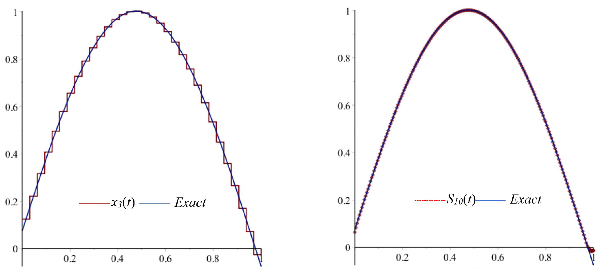
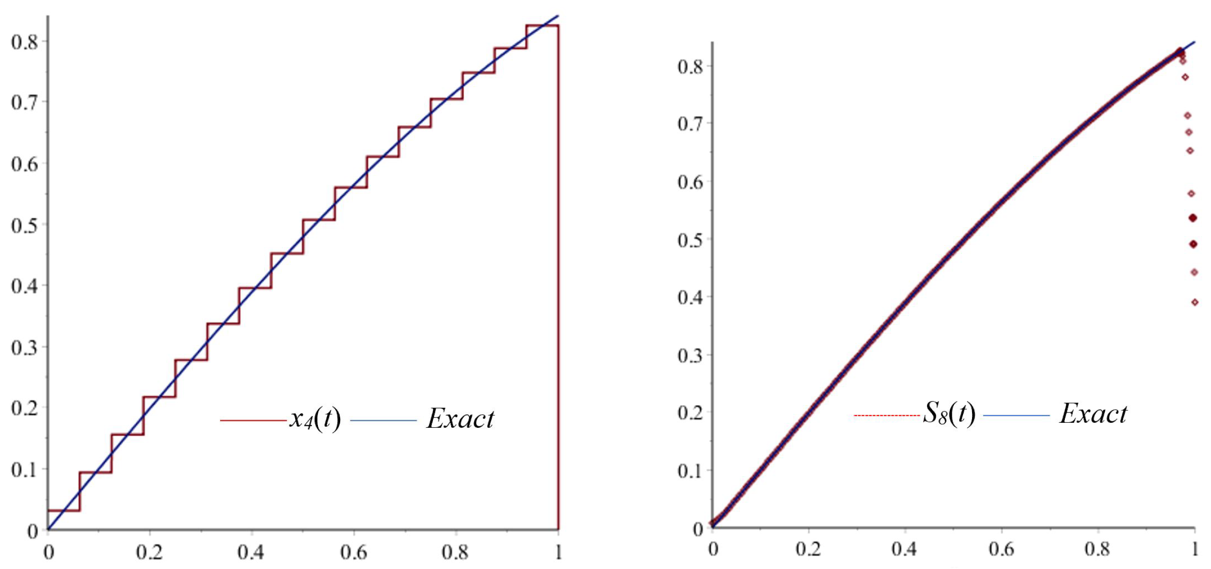
7. Numerical Examples

In this section, we demonstrate the efficiency of the Newton–Kantorovich-Haar wavelets method to solve nonlinear Fredholm and Volterra integral equations of the second kind. The calculation for each of these examples was performed in Maple 15.

Example 1.

Consider the following nonlinear Fredholm integral equation [11]

$$x\left(t\right)=sin\left(\pi t\right)+\frac{1}{5}{\int }_0^{1}cos\left(\pi t\right)sin\left(\pi s\right){\left(x\left(s\right)\right)}^{3}ds.$$

In order to approximate this integral equation, we repeat the Haar wavelets method until $x_3\left(t\right)$ and used the approach in Equation () to obtain $S_{10}\left(t\right)$.

We apply the same initial condition as $x_0\left(t\right)=0$ stated in [11] for $N=8$ and $N=16$. In

Table 1. Comparison of errors with the Newton–Kantorovich–Simpson quadrature method [11] for Example 1.

t	[11]	Presented Method	Presented Method
		${\mathit{S}}_{\mathbf{10}}\left(\mathit{t}\right),\mathit{N}=\mathbf{8}$	${\mathit{S}}_{\mathbf{10}}\left(\mathit{t}\right),\mathit{N}=\mathbf{16}$
0	4.98 × 10${}^{-2}$	1.38 × 10${}^{-2}$	1.13 × 10${}^{-3}$
0.05	4.92 × 10${}^{-2}$	1.41 × 10${}^{-3}$	5.85 × 10${}^{-4}$
0.1	4.74 × 10${}^{-2}$	2.75 × 10${}^{-4}$	1.96 × 10${}^{-4}$
0.15	4.44 × 10${}^{-2}$	4.15 × 10${}^{-3}$	9.23 × 10${}^{-4}$
0.2	4.03 × 10${}^{-2}$	2.70 × 10${}^{-3}$	21.51 × 10${}^{-3}$
0.25	3.52 × 10${}^{-2}$	1.75 × 10${}^{-3}$	6.49 × 10${}^{-5}$
0.3	2.93 × 10${}^{-2}$	4.53 × 10${}^{-3}$	5.63 × 10${}^{-4}$
0.35	2.26 × 10${}^{-2}$	3.80 × 10${}^{-3}$	1.01 × 10${}^{-3}$
0.4	1.54 × 10${}^{-2}$	5.14 × 10${}^{-3}$	1.26 × 10${}^{-3}$
0.45	7.80 × 10${}^{-3}$	4.77 × 10${}^{-3}$	1.28 × 10${}^{-3}$
0.5	0	5.05 × 10${}^{-3}$	1.32 × 10${}^{-3}$
0.55	0.780 × 10${}^{-3}$	4.52 × 10${}^{-3}$	1.38 × 10${}^{-3}$
0.6	1.54 × 10${}^{-2}$	5.10 × 10${}^{-3}$	1.23 × 10${}^{-3}$
0.65	2.26 × 10${}^{-2}$	3.12 × 10${}^{-3}$	8.53 × 10${}^{-4}$
0.7	2.93 × 10${}^{-2}$	4.04 × 10${}^{-3}$	3.08 × 10${}^{-4}$
0.75	3.52 × 10${}^{-2}$	5.39 × 10${}^{-3}$	1.93 × 10${}^{-3}$
0.8	4.03 × 10${}^{-2}$	1.86 × 10${}^{-3}$	1.39 × 10${}^{-3}$
0.85	4.44 × 10${}^{-2}$	3.41 × 10${}^{-3}$	7.29 × 10${}^{-4}$
0.9	4.74 × 10${}^{-2}$	7.29 × 10${}^{-4}$	4.96 × 10${}^{-5}$
0.95	4.92 × 10${}^{-2}$	2.60 × 10${}^{-3}$	8.46 × 10${}^{-4}$
1	4.98 × 10${}^{-2}$	8.66 × 10${}^{-2}$	6.27 × 10${}^{-2}$

, we compare the absolute error of the proposed method with those from Newton–Kantorovich–Simpson quadrature method [11]. Figure 1 shows the comparison of the approximated solution $x_3\left(x\right)$, $S_{10}\left(t\right)$ and the exact solution of this integral equation $x\left(t\right)=sin\left(\pi t\right)+\frac{1}{3}(20-\sqrt{391})cos\left(\pi t\right)$. The advantage of the proposed method is that we can obtain an estimate of all t values in the interval $\left[0,1\right]$ for any value of N, unlike the [11] method which can only obtain a certain t value depending on the subinterval number they divide.

Example 2.

Consider the following nonlinear Volterra integral equation [11]

$$x\left(t\right)-{\int }_0^t{x}^2\left(s\right)ds=sin\left(x\right)-\frac{t}{2}+\frac{1}{4}sin\left(2x\right).$$

For this example, we intend to solve the nonlinear Volterra integral equation by choosing the initial $x_0\left(t\right)=1$. In this case, we use four iterations to get the estimated settlement of $x_4\left(t\right)$ in Figure 2. In

Table 2. Comparison of errors with the Newton–Kantorovich–block-by-block method [11] for Example 2.

Nodes t	[11]	Presented Method	Presented Method
		${\mathit{S}}_{\mathbf{10}}\left(\mathit{t}\right),\mathit{N}=\mathbf{8}$	${\mathit{S}}_{\mathbf{8}}\left(\mathit{t}\right),\mathit{N}=\mathbf{16}$
0	0	1.61 × 10${}^{-2}$	8.29 × 10${}^{-3}$
$0.05$	4.16 × 10${}^{-5}$	4.52 × 10${}^{-4}$	7.31 × 10${}^{-4}$
$0.1$	3.33 × 10${}^{-4}$	5.98 × 10${}^{-4}$	4.40 × 10${}^{-4}$
$0.15$	7.90 × 10${}^{-4}$	5.55 × 10${}^{-4}$	7.66 × 10${}^{-4}$
$0.2$	1.54 × 10${}^{-3}$	2.26 × 10${}^{-4}$	2.79 × 10${}^{-6}$
$0.25$	3.93 × 10${}^{-3}$	9.88 × 10${}^{-4}$	3.78 × 10${}^{-4}$
$0.3$	6.65 × 10${}^{-3}$	1.37 × 10${}^{-4}$	4.69 × 10${}^{-4}$
$0.35$	8.87 × 10${}^{-3}$	6.11 × 10${}^{-4}$	3.00 × 10${}^{-4}$
$0.4$	1.39 × 10${}^{-2}$	4.67 × 10${}^{-4}$	7.69 × 10${}^{-4}$
$0.45$	1.97 × 10${}^{-2}$	2.60 × 10${}^{-4}$	7.84 × 10${}^{-5}$
$0.5$	0	9.34 × 10${}^{-4}$	7.31 × 10${}^{-4}$
$0.55$	3.53 × 10${}^{-2}$	1.08 × 10${}^{-4}$	5.60 × 10${}^{-4}$
$0.6$	4.70 × 10${}^{-2}$	5.30 × 10${}^{-4}$	7.68 × 10${}^{-5}$
$0.65$	5.47 × 10${}^{-2}$	4.15 × 10${}^{-4}$	8.85 × 10${}^{-4}$
$0.7$	6.90 × 10${}^{-2}$	2.17 × 10${}^{-4}$	1.84 × 10${}^{-4}$
$0.75$	8.45 × 10${}^{-2}$	7.98 × 10${}^{-4}$	3.56 × 10${}^{-4}$
$0.8$	9.59 × 10${}^{-2}$	3.31 × 10${}^{-5}$	6.48 × 10${}^{-4}$
$0.85$	1.19 × 10${}^{-1}$	5.23 × 10${}^{-4}$	1.47 × 10${}^{-4}$
$0.9$	1.43 × 10${}^{-1}$	1.80 × 10${}^{-4}$	6.48 × 10${}^{-4}$
$0.95$	1.60 × 10${}^{-1}$	1.73 × 10${}^{-2}$	3.22 × 10${}^{-4}$
1	1.85 × 10${}^{-1}$	4.42 × 10${}^{-1}$	4.51 × 10${}^{-1}$

, we compare the absolute error of the proposed method with Newton–Kantorovich block-by-block methods [11]. The exact solution for the integral equation is $sin\left(t\right).$

Example 3.

Consider the following nonlinear Fredholm integral equations [9]

$$x\left(t\right)+{\int }_0^1{e}^{t-2s}{\left[x\left(s\right)\right]}^{3}ds=e^{t+1}.$$

We solve the Fredholm integral equation by choosing the initial condition $x_0\left(t\right)=1.$ The approximated solution $x_3\left(t\right)$ is then converted to $S_{10}$ to obtain better accuracy for $N=4$. For the case of $N=8$, an adequate solution is obtained using a single iteration $x_1\left(t\right)$ but with a slight alteration where the approximated solution, $x_3\left(t\right)$ for $N=4$ is taken as the new initial condition. Similarly, we attain $x_1\left(t\right),$ for $N=16$ using the initial condition $x_1\left(t\right)$ of $N=8$.

Table 3. Comparison of errors with the Haar wavelet method [9] for Example 3.

Nodes t	[9],	Presented Method	Presented Method	Presented Method
	$\mathit{N}=\mathbf{16}$	${\mathit{S}}_{\mathbf{10}}\left(\mathit{t}\right),\mathit{N}=\mathbf{4}$	${\mathit{S}}_{\mathbf{10}}\left(\mathit{t}\right),\mathit{N}=\mathbf{8}$	${\mathit{S}}_{\mathbf{10}}\left(\mathit{t}\right),\mathit{N}=\mathbf{16}$
$0.1$	2.05 × 10${}^{-3}$	3.53 × 10${}^{-3}$	1.94 × 10${}^{-3}$	4.31 × 10${}^{-4}$
$0.2$	3.30 × 10${}^{-3}$	4.44 × 10${}^{-3}$	1.67 × 10${}^{-3}$	3.32 × 10${}^{-7}$
$0.3$	8.69 × 10${}^{-3}$	1.71 × 10${}^{-3}$	1.32 × 10${}^{-3}$	7.91 × 10${}^{-4}$
$0.4$	1.69 × 10${}^{-2}$	4.23 × 10${}^{-3}$	8.69 × 10${}^{-4}$	2.92 × 10${}^{-4}$
$0.5$	1.87 × 10${}^{-2}$	7.27 × 10${}^{-3}$	3.54 × 10${}^{-3}$	1.29 × 10${}^{-3}$
$0.6$	1.17 × 10${}^{-2}$	3.78 × 10${}^{-3}$	3.20 × 10${}^{-3}$	7.11 × 10${}^{-4}$
$0.7$	2.93 × 10${}^{-3}$	7.32 × 10${}^{-3}$	2.75 × 10${}^{-3}$	5.49 × 10${}^{-7}$
$0.8$	8.08 × 10${}^{-3}$	2.82 × 10${}^{-3}$	2.17 × 10${}^{-3}$	1.30 × 10${}^{-3}$
$0.9$	2.16 × 10${}^{-2}$	3.19 × 10${}^{-2}$	1.43 × 10${}^{-3}$	4.81 × 10${}^{-4}$

shows the absolute error using the Haar wavelets method [9] and the presented method. It is evident in Table 3 that our method is better than the Haar wavelets method [9] for this problem. Moreover, the presented method yields good estimation results with only $N=4$ compared to the Haar [9] method using $N=16$.

Example 4.

Consider the following nonlinear Fredholm integral equation [9]

$$x\left(t\right)-{\int }_0^{1}ts{\left[x\left(s\right)\right]}^{3}ds=e^t-\frac{(1+2e^3)t}{9},$$

in which the exact solution is $x\left(t\right)=e^t.$ In this example, we acquire an approximated solution of $x_3\left(t\right)$ using $N=4$ and by letting the initial condition $x_0\left(t\right)=1+x.$ Next, the first iterations for $N=8$ and $N=16$ are attained in similar manner as Example 3.

Table 4. Comparison of errors with the Haar wavelet method [9] for Example 4.

Nodes t	[9],	Presented Method	Presented Method	Presented Method
	$\mathit{N}=\mathbf{16}$	${\mathit{S}}_{\mathbf{10}}\left(\mathit{t}\right),\mathit{N}=\mathbf{4}$	${\mathit{S}}_{\mathbf{10}}\left(\mathit{t}\right),\mathit{N}=\mathbf{8}$	${\mathit{S}}_{\mathbf{10}}\left(\mathit{t}\right),\mathit{N}=\mathbf{16}$
$0.1$	9.46 × 10${}^{-3}$	3.05 × 10${}^{-3}$	9.42 × 10${}^{-4}$	1.96 × 10${}^{-4}$
$0.2$	5.36 × 10${}^{-3}$	4.56 × 10${}^{-3}$	1.31 × 10${}^{-3}$	2.53 × 10${}^{-4}$
$0.3$	4.40 × 10${}^{-3}$	5.03 × 10${}^{-3}$	1.61 × 10${}^{-3}$	5.22 × 10${}^{-4}$
$0.4$	1.16 × 10${}^{-2}$	6.86 × 10${}^{-3}$	1.79 × 10${}^{-3}$	4.73 × 10${}^{-4}$
$0.5$	2.30 × 10${}^{-2}$	9.23 × 10${}^{-3}$	3.13 × 10${}^{-3}$	9.42 × 10${}^{-4}$
$0.6$	1.67 × 10${}^{-2}$	8.92 × 10${}^{-3}$	3.40 × 10${}^{-3}$	8.11 × 10${}^{-4}$
$0.7$	8.37 × 10${}^{-3}$	1.18 × 10${}^{-2}$	3.54 × 10${}^{-3}$	5.42 × 10${}^{-4}$
$0.8$	2.40 × 10${}^{-3}$	1.04 × 10${}^{-2}$	3.55 × 10${}^{-3}$	1.31 × 10${}^{-3}$
$0.9$	1.59 × 10${}^{-2}$	3.41 × 10${}^{-3}$	3.38 × 10${}^{-3}$	8.46 × 10${}^{-4}$

describes both the absolute errors for the presented method $S_{10}\left(t\right)$ and Haar wavelets method [9].

Example 5.

Consider the following nonlinear Volterra integral equation [21]

$$x\left(t\right)+{\int }_0^t(x^2\left(s\right)+x\left(s\right))ds=\frac{3}{2}-\frac{1}{2}{e}^{-2t}.$$

with exact solution $e^{-t}.$ The initial guess is $x_0\left(t\right)=1$ in finding the approximate solution $x_4\left(t\right)$ and we use the same procedure as the example above in finding the approximate solution for $N=8$ and $N=16$. In

Table 5. Comparison of errors with the Haar wavelet method [21] for Example 5.

Nodes t	[21]	Presented Method	Presented Method	Presented Method
		${\mathit{S}}_{\mathbf{10}}\left(\mathit{t}\right),\mathit{N}=\mathbf{4}$	${\mathit{S}}_{\mathbf{10}}\left(\mathit{t}\right),\mathit{N}=\mathbf{8}$	${\mathit{S}}_{\mathbf{10}}\left(\mathit{t}\right),\mathit{N}=\mathbf{16}$
0	0	2.87 × 10${}^{-2}$	1.54 × 10${}^{-2}$	7.90 × 10${}^{-3}$
$0.1$	8.33 × 10${}^{-4}$	3.73 × 10${}^{-2}$	4.79 × 10${}^{-3}$	2.33 × 10${}^{-4}$
$0.2$	3.75 × 10${}^{-4}$	1.41 × 10${}^{-2}$	5.52 × 10${}^{-3}$	1.28 × 10${}^{-5}$
$0.3$	1.11 × 10${}^{-3}$	5.86 × 10${}^{-3}$	5.54 × 10${}^{-3}$	4.25 × 10${}^{-4}$
$0.4$	3.51 × 10${}^{-4}$	2.06 × 10${}^{-2}$	3.27 × 10${}^{-3}$	3.64 × 10${}^{-7}$
$0.5$	5.80 × 10${}^{-4}$	2.73 × 10${}^{-3}$	8.20 × 10${}^{-7}$	1.19 × 10${}^{-4}$
$0.6$	1.32 × 10${}^{-4}$	2.27 × 10${}^{-2}$	2.84 × 10${}^{-3}$	7.97 × 10${}^{-6}$
$0.7$	4.95 × 10${}^{-4}$	9.48 × 10${}^{-3}$	3.19 × 10${}^{-3}$	2.41 × 10${}^{-4}$
$0.8$	1.73 × 10${}^{-4}$	3.00 × 10${}^{-3}$	3.67 × 10${}^{-3}$	2.74 × 10${}^{-5}$
$0.9$	3.68 × 10${}^{-4}$	1.41 × 10${}^{-2}$	1.68 × 10${}^{-3}$	2.56 × 10${}^{-4}$

, we compare the absolute error of the proposed method with hybrid Taylor polynomials and Block-Pulse functions [21].

8. Conclusions

This study describes new techniques using a combination of Newton–Kantrovich and Haar wavelets to solve the second kind of nonlinear Fredholm and Volterra integral equations. It has been proven that an appropriate initial guess is required in the Newton–Kantrovich method. Therefore, when applying large values of N such as $N=16$ to the approximation of the Haar wavelets $x_{16}\left(t\right)$, we recommend using the previous approximate solution $x_8\left(t\right)$ or $x_4\left(t\right)$ which considers the smaller value of N as an initial condition. This will ultimately reduce the number of iterations and improve the accuracy of the estimated solution. We also provide a simple approach at the end of Section 4 and Section 5 that can improve the approximation solution without increasing the number of bases N for the functions of Haar wavelets.

References

1. Liu, Y. Application of the Chebyshev polynomial in solving Fredholm integral equations. Math. Comput. Model. 2009, 50, 465–469. [Google Scholar] [CrossRef]
2. Babaaghaie, A.; Maleknejad, K. A new approach for numerical solution of two-dimensional nonlinear Fredholm integral equations in the most general kind of kernel, based on Bernstein polynomials and its convergence analysis. J. Comput. Appl. Math. 2018, 344, 482–494. [Google Scholar] [CrossRef]
3. Capobianco, G.; Conte, D.; Del Prete, I. High performance parallel numerical methods for Volterra equations with weakly singular kernels. J. Comput. Appl. Math. 2009, 228, 571–579. [Google Scholar] [CrossRef] [Green Version]
4. Golbabai, A.; Keramati, B. Solution of non-linear Fredholm integral equations of the first kind using modified homotopy perturbation method. Chaos Solitons Fractals 2009, 39, 2316–2321. [Google Scholar] [CrossRef]
5. Yousefi, S.; Razzaghi, M. Legendre wavelets method for the nonlinear Volterra–Fredholm integral equations. Math. Comput. Simul. 2005, 70, 1–8. [Google Scholar] [CrossRef]
6. Aziz, I. New algorithms for the numerical solution of nonlinear Fredholm and Volterra integral equations using Haar wavelets. J. Comput. Appl. Math. 2013, 239, 333–345. [Google Scholar] [CrossRef]
7. Mohammadi, F.A. Chebyshev wavelet operational method for solving stochastic Volterra-Fredholm integral equations. Int. J. Appl. Math. Res. 2015, 4, 217. [Google Scholar] [CrossRef] [Green Version]
8. Aziz, I.; Al-Fhaid, A.S. An improved method based on Haar wavelets for numerical solution of nonlinear integral and integro-differential equations of first and higher orders. J. Comput. Appl. Math. 2014, 260, 449–469. [Google Scholar]
9. Babolian, E.; Shahsavaran, A. Numerical solution of nonlinear Fredholm integral equations of the second kind using Haar wavelets. J. Comput. Appl. Math. 2009, 225, 87–95. [Google Scholar] [CrossRef] [Green Version]
10. Maleknejad, K.; Almasieh, H.; Roodaki, M. Triangular functions (TF) method for the solution of nonlinear Volterra–Fredholm integral equations. Commun. Nonlinear Sci. Numer. Simul. 2010, 15, 3293–3298. [Google Scholar] [CrossRef]
11. Saberi-Nadjafi, J.; Heidari, M. Solving nonlinear integral equations in the Urysohn form by Newton–Kantorovich–quadrature method. Comput. Math. Appl. 2010, 60, 2058–2065. [Google Scholar] [CrossRef] [Green Version]
12. Appell, J.; De Pascale, E.; Zabrejko, P.P. On the application of the Newton-Kantorovich method to nonlinear integral equations of Uryson type. Numer. Funct. Anal. Optim. 1991, 12, 271–283. [Google Scholar] [CrossRef]
13. Appell, J.; De Pascale, E.; Lysenko, J.V.; Zabrejko, P.P. New results on Newton-Kantorovich approximations with applications to nonlinear integral equations. Numer. Funct. Anal. Optim. 1997, 18, 1–17. [Google Scholar] [CrossRef]
14. Boikov, I.V.; Tynda, A.N. Approximate Solution of Nonlinear Integral Equations of the Theory of Developing Systems. Differ. Equ. 2003, 39, 1277–1288. [Google Scholar] [CrossRef]
15. Aziz, I.; Haq, F. A comparative study of numerical integration based on Haar wavelets and hybrid functions. Comput. Math. Appl. 2010, 59, 2026–2036. [Google Scholar]
16. Uko, L.U.; Argyros, I.K. A weak Kantorovich existence theorem for the solution of nonlinear equations. J. Math. Anal. Appl. 2008, 342, 909–914. [Google Scholar] [CrossRef] [Green Version]
17. Kantorovich, L.V. On Newton’s method for functional equations. Dokl. Akad. Nauk SSSR 1948, 59, 1237–1240. [Google Scholar]
18. Shen, W.; Li, C. Kantorovich-type convergence criterion for in exact Newton methods. Appl. Numer. 2009, 59, 1599–1611. [Google Scholar] [CrossRef]
19. Argyros, I.K. On Newton’s method for solving equations containing Fr’echet-differentiable operators of order at least two. Appl. Math. Comput. 2009, 215, 1553–1560. [Google Scholar]
20. Anvarjon, A. Ahmedov and Mohammad Hasan Abdul Sathar and Ahmad Fadly Nurullah Rasedee and Nor Fadzilah Binti Mokhtar. Approximating of functions from Holder classes Hα[0, 1]. by Haar wavelets. J. Phys. Conf. Ser. 2017, 890, 012073. [Google Scholar]
21. Sabzevari, M. A review on “Numerical solution of nonlinear Volterra-Fredholm integral equations using hybrid of.” 52 (2013) 551–555. Alex. Eng. J. 2019, 58, 1099–1102. [Google Scholar] [CrossRef]
Figure 1. Comparison of the approximated solution x 3 ( t ) and S 10 ( t ) for N = 16 with the exact solution for Example 1.
Symmetry 12 02034 g001
Figure 2. Comparison of the approximated solution x 4 ( t ) and S 8 ( t ) for N = 16 with the exact solution for Example 2.
Symmetry 12 02034 g002