Optimization of the Mixture Transition Distribution Model Using the March Package for R

Abstract

Optimization of mixture models such as the mixture transition distribution (MTD) model is notoriously difficult because of the high complexity of their solution space. The best approach comprises combining features of two types of algorithms: an algorithm that can explore as completely as possible the whole solution space (e.g., an evolutionary algorithm), and another that can quickly identify an optimum starting from a set of initial conditions (for instance, an EM algorithm). The march package for the R environment is a library dedicated to the computation of Markovian models for categorical variables. It includes different algorithms that can manage the complexity of the MTD model, including an ad hoc hill-climbing procedure. In this article, we first discuss the problems related to the optimization of the MTD model, and then we show how march can be used to solve these problems; further, we provide different syntaxes for the computation of other models, including homogeneous Markov chains, hidden Markov models, and double chain Markov models.

1. Introduction

Despite their long history and use in many scientific fields, Markovian models are difficult to apply in practice because of the lack of empirical tools. For instance, Markovian models are not included in the base versions of statistical environments such as SPSS, SAS, and Stata, and researchers need to either adopt a log-linear approach (for homogeneous Markov chains only) or rely on ad hoc toolboxes developed by third parties such as MARKOV [1] and mixmcm [2] for Stata, or PTRANSIT [3] and MARKOV [4] for SAS. Some specialized software programs such as Latent Gold [5] have been developed; however, they remain incomplete and are not open source. Recently, some researchers used the Julia language [6], but now the most used environment for Markovian computations is R [7] with packages such as depmixS4 [8] for continuous variables and markovchain [9] for categorical variables.

In addition to the well-known homogeneous Markov chain and hidden Markov models, many other Markovian models have been developed over the years. Among them, the mixture transition distribution (MTD) model proposed first by Raftery [10] is of great interest because it is considerably more parsimonious than the fully parameterized Markov chains. However, to the best of our knowledge, none of the above-mentioned software programs can estimate the MTD model for categorical variables. In fact, we know that only two pieces of software can deal with the MTD model: seqpp [11], which was developed in C++, but it is no longer available; and march for Windows [12], a standalone piece of software available for the Windows environment only, which is still available but whose development was definitively stopped in 2010. This lack of options when using the MTD model is not surprising, because similarly to other mixture models, this model is notoriously difficult to optimize. Therefore, there is a need for an R package dedicated to the computation of Markovian models for categorical variables and one that can handle the MTD model. We decided to rewrite the old march for Windows software (originally developed in the MATLAB language) as an R package and improve it. This package is freely available from CRAN (https://cran.r-project.org/).

The objectives of this paper are (1) to describe the difficulties occurring when optimizing the MTD model; (2) to demonstrate how to overcome these difficulties using the R package march; (3) to show how the march package can be used to optimize other Markovian models.

The rest of this paper is organized as follows. Section 2 introduces the MTD model and its optimization details. In Section 3, we present the main features of the march package, and in Section 4, we consider the specific case of MTD models. Further, we provide a practical example in Section 5. An appendix provides additional syntax with which to optimize other Markovian models.

2. MTD Model and Its Optimization

Let $Y_t$ be a categorical random variable that takes values in the finite set $\{1,\dots ,c\}$. In an f-order MTD model, each lag of the random variable ($Y_{t-1},Y_{t-2},\dots ,Y_{t-f}$) influences $Y_t$ independently as

$$\begin{array}{ccc}\hfill P(Y_t=i_0|Y_{t-f}=i_f,\dots ,Y_{t-1}=i_1)& =& \sum _{g=1}^f{\lambda }_{g}P(Y_t=i_0|Y_{t-g}=i_g)\hfill \\ & =& \sum _{g=1}^f{\lambda }_g{q}_{i_g{i}_0},\hfill \end{array}$$

where

$$Q=\left(\begin{array}{ccc}{q}_{11}& \dots & q_{1c}\\ ⋮& & ⋮\\ q_{c1}& \dots & q_{cc}\end{array}\right)$$

represents a transition matrix, and where $({\lambda }_1,\dots ,{\lambda }_f)$, ${\sum }_i{\lambda }_i=1$, are the weights associated to each lag. The transition probabilities in the matrix Q and the weights associated with each lag are estimated by optimization of the log-likelihood of the model [13]. The MTDg model is a generalization of the MTD model wherein a different transition matrix, $Q_1$, $Q_2$, etc., is used to represent the link between each lag of the model and $Y_t$. Moreover, covariates can be added to the model [14]. For more details about the concept of the MTD model and its usefulness, readers can refer to the review article by Berchtold and Raftery [15].

Mixture models are notoriously difficult to optimize [16], and the MTD model is not an exception, especially when a different transition matrix is used for each lag and/or when covariates are added to the model. The problem arises from the fact that as the complexity of the model increases, the solution space can become very irregular, with many different local optima. Standard estimation algorithms such as the EM algorithm are very efficient in finding a solution; however, they are trapped inside the basin of attraction of one specific optimum. An ad hoc estimation algorithm belonging to the hill-climbing family was proposed for the MTD model [13]; however, even if this algorithm is efficient in most scenarios—similarly to the EM algorithm—it sometimes fails to identify the global optimum of the solution space because (1) the re-estimation of each parameter is considered separately, and (2) some parts of the solution space are not explored at all. These issues indicate that finding the global optimum is related to the set of initial conditions: If the starting point of the optimization process lies inside the basin of attraction of the global optimum, it will be found. Otherwise, the algorithm will converge to another (local) optimum.

To illustrate this point, we defined the following second-order MTDg model: The vector of the lag weights is

$$\Lambda =\left(\frac{{\theta }_1+{\theta }_2}{2}1-\frac{{\theta }_1+{\theta }_2}{2}\right),$$

and the transition matrices corresponding to the first and second lags are

$$Q_1=\left(\begin{array}{cc}{\theta }_1& 1-{\theta }_1\\ {\theta }_2& 1-{\theta }_2\end{array}\right)and{Q}_2=\left(\begin{array}{cc}1-0.8·{\theta }_2& 0.8·{\theta }_2\\ 1-0.5·{\theta }_1& 0.5·{\theta }_1\end{array}\right).$$

The model was applied to a dataset of n = 845 sequences of length 13 of a dichotomous variable using the hill-climbing optimization algorithm. Refer to Section 5 for a description of the dataset.

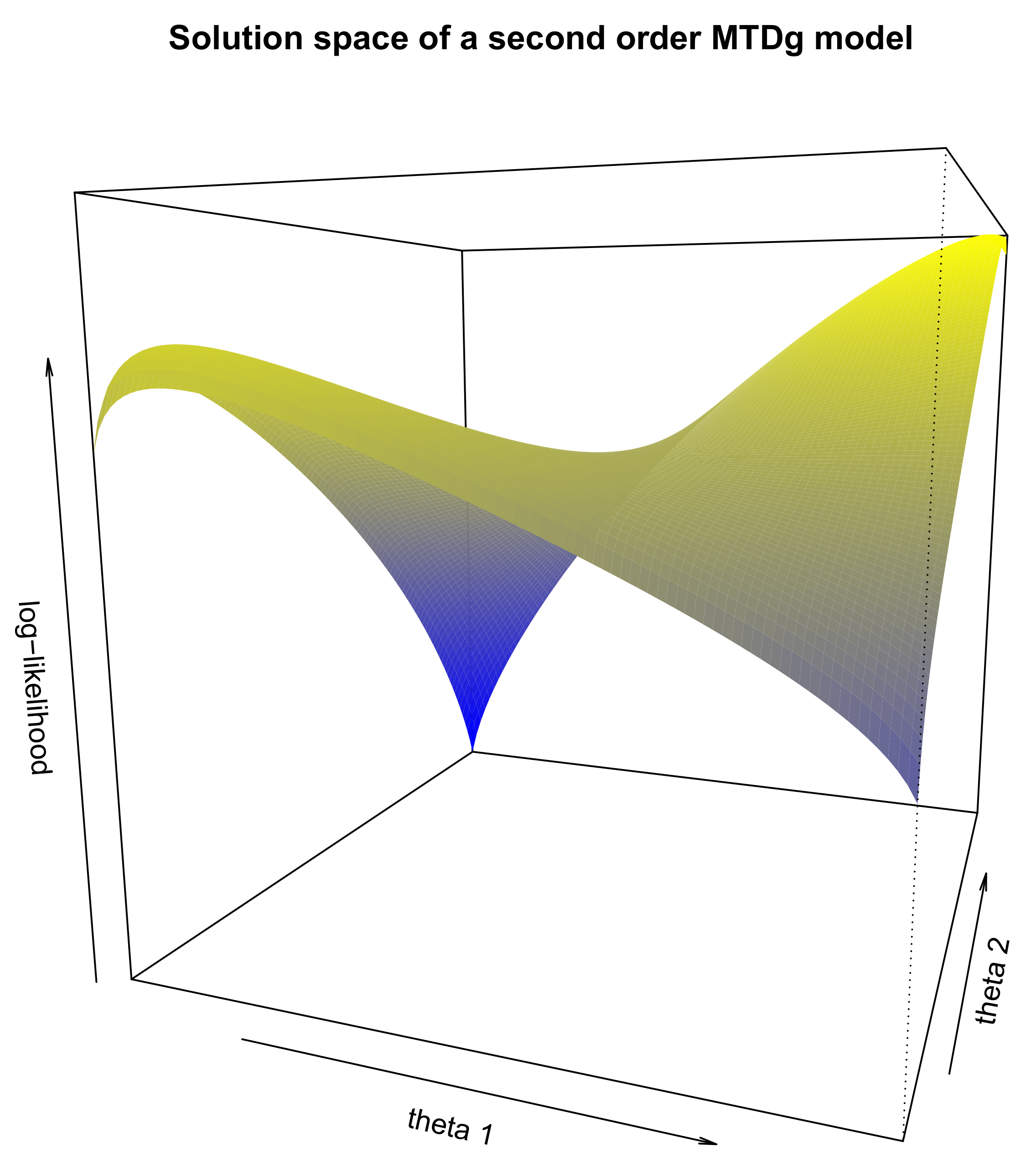
Figure 1 shows the solution space of this model for all combinations of ${\theta }_1=(0.01,\dots ,0.99)$ and ${\theta }_2=(0.01,\dots ,0.99)$. We can see that there are two optima, a local one on the left and the global one on the right. If we optimize the MTDg model starting from each point on the figure and by applying the HC algorithm [13], the model will then converge to two different values of the log-likelihood, −3348.3 corresponding to the local optimum and −2057.9 corresponding to the global one. Therefore, converging to the global optimum rather than to the local optimum depends on the starting point of the optimization algorithm.

The above example is not fully realistic because it involves a model with many constraints on its parameters; however, these constraints were necessary to visualize the solution space. Despite this limitation, this example correctly illustrates the types of issues that occur with mixture models. It is absolutely necessary to explore the entire solution space to identify the basin of attraction of the global maximum, and thereby, the global maximum itself.

Different solutions to the exploration of the solution space problem were proposed in the literature, either based on a modification of the standard EM algorithm to allow it to escape from a specific basin of attraction (e.g., SEM, CEM [17]), or based on a better exploration of the entire solution space. In the second category, we find that different nature-inspired optimization algorithms, i.e., algorithms that attempt to mimic life or genetic behaviors, for instance, by recombining different potential solutions, allow the emergence of even better solutions [18]. These evolutionary algorithms have the theoretical capacity to explore the solution space of a problem fully to identify its global optimum. However, the drawback is that they can be extremely slow to converge. Therefore, a good solution is to perform two-step optimization. In the first step, an evolutionary algorithm is used to identify the region of the solution space that contains the optimum, and in the second step, a faster algorithm is used to converge to this optimum. Such an approach is feasible in the case of the MTD model by combining the different algorithms implemented in the march package.

3. Main Features of the march Package

As noted before, there remains a lack of available software for the computation of Markovian models adapted to categorical variables. The march package for R was developed to fill this gap. It was developed around the double chain Markov model (DCMM) [19,20], a general framework that includes many different Markovian models. This framework is characterized by a two-level approach similar to a standard hidden Markov model, but with a direct link between successive observations of the visible variable Y, which is similar to standard homogeneous Markov chains (Figure 2). The DCMM model is a method of modeling heterogeneous observed behaviors; however, this framework is sufficiently flexible to include many other specific models as subcases. For instance, by removing the direct link between successive values of the observed variable, the DCMM becomes a standard HMM. By allowing only one state for the hidden variable X, we suppress the influence of this latent process upon the visible level, transforming the DCMM into a homogeneous Markov chain. By constraining the hidden transition matrix with the identity matrix, the DCMM becomes a clustering tool. If we consider dependence orders larger than one for either the hidden process or the visible one, then we can also replace these processes with MTD modelings. Finally, covariates can also be included at both levels.

Three different optimization algorithms are implemented in the march package, and they can be combined to improve the speed of convergence and the quality of the solution. First, the DCMM is traditionally optimized using the Baum–Welch algorithm, a customized version of the EM algorithm [19]. In particular, to fulfill all constraints inherent to the model, we implemented a general EM (GEM) algorithm, which is an EM algorithm in which the M-step ensures a monotonous increase in the log-likelihood but not necessarily the best possible improvement of the log-likelihood [21].

The second optimization algorithm is an evolutionary algorithm (EA) that can be used to better explore the solution space of complex models [18]. Starting from an initial randomly generated population of possible solutions, new generations of the population are built by applying three different operators: simulated binary crossover [22], Gaussian mutation, and fitness proportional selection [23]. Each possible solution is evaluated using a measure of its fitness, defined as −1/log-likelihood. The algorithm itself is a Lamarckian EA, where a new generation is potentially composed of children and parents. In particular, if $PopSize$ denotes the size of the population, the following operations are performed to build the next generation:

• Two members of the current population are randomly selected, and their probabilities of selection are proportional to their fitness values.
• A random crossover occurs between the two selected members of the population with a probability that can be selected by the user (default: 50%). This operation leads to two children solutions.
• A mutation is applied to the two children by adding a Gaussian distributed noise to each parameter with a probability that can be chosen by the user (default: 5%).
• The two children are improved using the GEM algorithm, with a number of iterations that can be chosen by the user (default: 2).
• The fitness of each children is computed.

The five steps above are repeated until the size of the children’s population equals that of the parent population. Then, the populations of parents and children are aggregated, and a reduction operation is applied to return to the original population size. $PopSize$ solutions are selected randomly to constitute the new generation, with probabilities of selection proportional to their fitness values. The algorithm then iterates to build the next generation until the planned number of iterations is reached.

By using fitness proportional selection, we allow that in some cases none of the best current members of the population are selected. This provides the algorithm a better capability to explore the full solution space. Simulated binary crossover and Gaussian mutation are also helpful in dealing with the real-valued genome representation, which is used to encode the different parameters of the DCMM. Indeed, using bit-flip operations would induce problems in bit-encoded real values; for instance, mutating the sign bit of a number creates a very different individual. The user can choose to suppress some parts of the above algorithm by setting the crossover probability, mutation probability, or number of GEM iterations to zero.

Combining the two previous optimization algorithms, a typical estimation procedure for the DCMM consists of the following two steps:

• The EA algorithm is used to identify a candidate solution in the attraction basin of the global optimum.
• Starting from this candidate solution, the GEM algorithm is used to optimize the model until reaching the global optimum.

The third estimation algorithm included in march specifically concerns the MTD model and comprises an implementation of the ad hoc hill-climbing (HC) algorithm proposed by Berchtold [13]. This HC algorithm is used in two different manners within march: On the one hand, when the MTD model is viewed as a special case of the DCMM, it is estimated with the EA + GEM algorithm, and in this case, the HC algorithm is part of the GEM algorithm. On the other hand, when a MTD model is defined directly, without reference to the DCMM framework, the HC algorithm is used directly to compute the model. The main difference between the two cases is that in the first case, the HC algorithm is reinitialized at the beginning of each iteration of the GEM algorithm to account for the possible other changes performed by the algorithm. In contrast, when used independently of the DCMM framework, the HC algorithm is initialized only once, and then it runs until reaching an optimum. Therefore, depending on the context of use, the HC algorithm can possibly lead to different (local) optima of the solution space.

In addition to being able to optimize many models within the DCMM framework, and to have a dedicated function for the MTD model, the march package includes optimized functions for the computation of the independence model, of homogeneous Markov chains of any order, of confidence intervals, and of the Akaike and Bayesian information criteria. Moreover, covariates can be added to most models, even if the resulting models are no longer Markovian.

4. Combining Estimation Algorithms for the MTD Model

The march package includes three different algorithms (EA, GEM, and HC) that can be used to optimize an MTD model, and these algorithms can be combined for improved efficiency. Therefore, we suggest the following approach:

• Optimize the MTD model of interest using the HC algorithm with standard parameter values. If the model is sufficiently simple and if it is likely to have only one global optimum and no local ones, then this algorithm will find the optimum value very quickly. Otherwise, it could provide a good idea for the structure of the solution.
• Use the EA algorithm to perform a more complete search of the solution space to identify possible solutions that could have been missed by the HC algorithm because they do not belong to the same basin of attraction.
• Optimize the best solution fond by the EA algorithm using the HC algorithm either within the GEM algorithm or independently of it.

A solution that is found after applying step 3 will often be similar to that of point 1; however, it can sometimes be different, and the more complex the solution space, the more likely they will differ. Moreover, other possibilities including optimization based on the sole GEM or EA algorithms exist.

In many scenarios, the exact structure of the best MTD model is not known in advance, and it will need to be selected as a function of the analyzed dataset. For instance, it may not be known which dependence order will fit the data more accurately, and whether a single transition matrix should be used for each lag or if it is more suitable to use as many matrices as lags, or whether the addition of covariates to the model will improve it. Different optimization algorithms available in march can optimize a specific MTD model, but they cannot compare different specifications of the MTD model automatically. Therefore, when unsure about the best specification of the model, it is necessary to separately optimize each possible specification of the model before deciding which one is the most appropriate. In addition to the log-likelihood that is available for each model, it is recommended to use the AIC and BIC criteria to compare these different models [24].

An important point when comparing different models is to ensure that each model is computed on the same subsample of the dataset. For instance, if the Markov chains of orders one and two are computed on a sequence of n = 100 data points, then 99 transitions are available for computing the first-order model, but only 98 for the second-order model. Therefore, the log-likelihood of the two models and the models themselves are not fully comparable. In such a scenario, the solution is to fix a maximal order for the computation of all models, and then compute each model as a function of this maximal order. The parameter maxOrder that is available in all optimization functions in march allows the researcher to compute models that are all comparable. In the previous example, if maxOrder is set to 2, then the a second-order Markov chain will be computed using data points 1 to 100, and the first-order model will be computed using data points 2 to 100. In both cases, exactly 98 transitions will be used to estimate the model and compute its log-likelihood.

5. Example

We used the Employment.2 dataset, which has been included in the march package since version 3.2.5. This dataset contains n = 845 sequences of the 13 successive observations of a categorical variable representing the professional activity categorized into two categories: 1 = “Full time employee”; 2 = “Other situation”. The first observation of each sequence corresponds to the status of the respondent at age 20, and then the following data were observed every two years, the last observation corresponding to the status at age 44. In addition, two covariates were also provided in the dataset. The first one is a fixed covariate representing gender (1 = “Female”; 2 = “Male”), and the second one is a time-varying covariate representing health status (1 = “Good”; 2 = “Bad”). The example discussed in Section 2 was based on the same dataset.

We considered a second-order MTDg model, which is a model whose current observation is explained by the last two observations, and in which two different transition matrices are used to represent the relationship between each of the two lags and the present. Further, we included the gender and health covariates in the model. This model was chosen for the convenience of the presentation, and it is not necessarily the best model to explain the dataset. This question is beyond the scope of the present article.

To find the best solution of the model in terms of statistical criteria, the first possibility is to rely on the sole HC algorithm by using the syntax:

 set.seed(1234)

 Model.1 <- march.mtd.construct(Employment.2,order=2, MCovar=c(1,1), init="best",

                                mtdg=T, llStop=0.0001, maxIter = 1000, maxOrder=2)

 print(Model.1)

 march.BIC(Model.1)

In the above code, the set.seed(1234) command is used to allow reproducible results by setting the R random generator to a specific point (here: 1234). Using another seed is likely to produce slightly different results. The march.mtd.construct() function is used to define the model and then optimize it using the pure HC algorithm. The march.BIC() command computes the Bayesian information criterion of the solution. We obtained a log-likelihood of −1813.737 for 10 independent parameters and a BIC value of 3718.846.

In the above syntax, the init= "best" option means that the initial transition matrix between each lag of the MTDg model and the present is the corresponding empirical transition matrix computed from the entire dataset. The use of another seed would not change that, but another possibility is to use the init="random" option that replace the empirical transition matrices by randomly created transition matrices as the starting points of the optimization procedure. In practice, using the init="random" option with seed 1234 did not change the results, and the same was observed with other seeds such as 233 and 984. Other options used in the march.mtd.construct function indicate that the model is an MTDg rather than an MTD model (mtdg = T); the algorithm will stop when the difference in the log-likelihood between two successive iterations is below 0.0001 (llStop = 0.0001); the maximal number of iterations of the algorithm is fixed to 1000 (maxIter = 1000); and the model is computed considering a maximal possible order of two for comparison with other model specifications (maxOrder = 2).

A second possibility is to estimate the model using the GEM algorithm. Using the following syntax,

 set.seed(1234)

 Model.2 <- march.dcmm.construct(Employment.2, orderHC=1, orderVC=2, M=1,

                                 gen=1, popSize=1, iterBw=100, stopBw = 0.01,

                                 CMCovar=c(1,1), Cmodel="mtdg", maxOrder=2)

 print(Model.2)

 march.BIC(Model.2)

we obtained a log-likelihood of −1813.782 for 10 independent parameters and a BIC value of 3718.935. Here, we allowed for a maximum of 100 iterations of the algorithm (iterBw = 100), and the algorithm had to stop whenever the difference in log-likelihood between two successive iterations became lower than 0.01 (stopBw = 0.01). Moreover, the options gen = 1 and popSize = 1 ensured that only the GEM part of the function was used, completely bypassing the evolutionary algorithm.

A third option is to first explore the solution space using an evolutionary algorithm before optimizing the best candidate using either the GEM or HC algorithm. The following syntax starts a search in the entire solution space with a population of 20 candidate solutions and 20 iterations of the EA algorithm:

 set.seed(1234)

 Model.3 <- march.dcmm.construct(Employment.2, orderHC=1, orderVC=2, M=1,

                                 gen=20, popSize=20, pMut=0.05, pCross=0.5, iterBw=0,

                                 CMCovar=c(1,1), Cmodel="mtdg", maxOrder=2)

 print(Model.3)

 march.BIC(Model.3)

In the above syntax, the crossover and mutation operators were allowed with respective probabilities 0.5 and 0.05; however, no improvement of children solutions with the GEM algorithm did occur (option iterBw = 0). As expected, the solution reached after this pure EA with a very limited number of generations (20) was far from optimal with a log-likelihood of −1895.900 for six independent parameters and a BIC value of 3846.624. However, it was possible to improve it, by using either the HC algorithm

 set.seed(1234)

 Model.3a <- march.mtd.construct(Employment.2, order=2, MCovar=c(1,1),

                                 mtdg=T, llStop=0.0001, maxIter = 1000, maxOrder=2,

                                 seedModel=Model.3)

 print(Model.3a)

 march.BIC(Model.3a)

or the GEM algorithm

 set.seed(1234)

 Model.3b <- march.dcmm.construct(Employment.2, orderHC=1, orderVC=2, M=1,

                                  gen=1, popSize=1, iterBw=100, stopBw = 0.01,

                                  CMCovar=c(1,1), Cmodel="mtdg", maxOrder=2,

                                  seedModel = Model.3)

 print(Model.3b)

 march.BIC(Model.3b)

In both of the above codes, the seedModel option indicates that the optimization must start from the model stored in the Model.3 object containing the best solution at the end of the EA algorithm. The HC algorithm then leads to a log-likelihood of −1818.598 for six independent parameters and a BIC value of 3692.019, when the GEM algorithm leads to a solution with a log-likelihood of −1813.955 for eight independent parameters and a BIC value of 3701.008.

As explained in Section 3, the exploration of the solution space by the EA algorithm can be improved when a few number of GEM iterations are applied to each child solution. This is performed by the following syntax. Compared to the syntax used for the Model.3, the iterBw option is now set to two iterations:

 set.seed(1234)

 Model.4 <- march.dcmm.construct(Employment.2, orderHC=1, orderVC=2, M=1,

                                 gen=20, popSize=20, pMut=0.05, pCross=0.5, iterBw=2,

                                 CMCovar=c(1,1), Cmodel="mtdg", maxOrder=2)

 print(Model.4)

 march.BIC(Model.4)

With this optimization procedure, we obtained a log-likelihood of −1813.735 for 11 independent parameters and a BIC value of 3727.979. Similarly to what was done for Model.3, we attempted to improve this solution by using either the HC algorithm or the GEM algorithm, but none of these algorithms could find a better solution. The results from the different optimization procedures are summarized in

Table 1. Main characteristics of the different Markovian models computed on the Employment.2 dataset. The first part of the table summarizes the second-order MTDg models with two covariates obtained from different optimization procedures, and the second part of the table summarizes the other Markovian models appearing in Appendix A. Regarding the different optimization procedures, HC means hill-climbing, GEM means general expectation-maximization algorithm, EA means evolutionary algorithm, and exact indicates that there is an exact solution to the maximization of the log-likelihood.

Model	Model	Optimization	Number of	Log-Likelihood	BIC
Name	Structure	Procedure	Parameters
Model.1	MTDg2 + cov	HC	10	−1813.737	3718.846
Model.2	MTDg2 + cov	GEM	10	−1813.782	3718.935
Model.3	MTDg2 + cov	EA	6	−1895.900	3846.624
Model.3a	MTDg2 + cov	EA + HC	6	−1818.598	3692.019
Model.3b	MTDg2 + cov	EA + GEM	8	−1813.955	3701.008
Model.4	MTDg2 + cov	EA/GEM	11	−1813.735	3727.979
Model.indep	Independence	exact	1	−6433.625	12876.390
Model.mc1	MC1	exact	2	−2064.818	4147.910
Model.mc2	MC2	exact	4	−2055.297	4147.193
Model.mtd2	MTD2	HC	3	−2057.873	4143.159
Model.mtdg2	MTDg2	HC	4	−2057.873	4152.296
Model.hmm2	HMM2	GEM	5	−2288.941	4623.568
Model.hmm3	HMM3	GEM	11	−2265.008	4630.526
Model.dcmm2	DCMM2	GEM	7	−2063.297	4190.555

.

To summarize, depending on the optimization procedure, we obtained different solutions with close log-likelihoods, but with different numbers of parameters and hence BIC values. The solution achieved by the pure HC algorithm reads

$$\Lambda =\left(0.7900.0350.1480.026\right),$$

(1a)

where the four weights correspond to the first and second lags, respectively, and to the Gender and Health covariates. The transition matrices corresponding to the first and second lags are

$$Q_1=\left(\begin{array}{cc}1& 0\\ 0.001& 0.999\end{array}\right)\mathrm{and}{Q}_2=\left(\begin{array}{cc}0.852& 0.148\\ 0.158& 0.842\end{array}\right),$$

(1b)

and the transition matrices corresponding to the two covariates are

$$Q_{Gender}=\left(\begin{array}{cc}0.017& 0.983\\ 0.955& 0.045\end{array}\right)\mathrm{and}{Q}_{Health}=\left(\begin{array}{cc}0.511& 0.489\\ 0.651& 0.349\end{array}\right).$$

(1c)

At the sample level, the four explanatory elements are all useful because their weights are all larger than zero; however, the first lag is clearly the most important explanatory element, followed by the Gender covariate.

The solution provided by the combination EA + HC reads

$$\Lambda =\left(0.85800.1410.001\right),$$

(2a)

$$Q_1=\left(\begin{array}{cc}0.971& 0.029\\ 0.031& 0.969\end{array}\right)\mathrm{and}{Q}_2=\left(\begin{array}{cc}0.481& 0.519\\ 0.528& 0.472\end{array}\right),$$

(2b)

$$Q_{Gender}=\left(\begin{array}{cc}0& 1\\ 0.998& 0.002\end{array}\right)\mathrm{and}{Q}_{Health}=\left(\begin{array}{cc}1& 0\\ 0.565& 0.435\end{array}\right).$$

(2c)

Contrarily to the solution given by parameters (1a)–(1c), the second lag is inactive (its weight is zero), and therefore, the corresponding transition matrix is not used, which explains in part the reduced number of parameters. Further, it can be noticed that the weight associated with the Health covariate is very small, and that it could be interesting to recompute the model without it. Moreover, the transition matrix associated with each covariate has a transition that is certain (with a probability of 1), what implies one less independent parameter for each matrix.

Finally, the solution given by the combination EA + GEM reads

$$\Lambda =\left(0.7980.0270.1760\right),$$

(3a)

$$Q_1=\left(\begin{array}{cc}0.991& 0.009\\ 0.003& 0.997\end{array}\right)\mathrm{and}{Q}_2=\left(\begin{array}{cc}0.977& 0.023\\ 0.059& 0.941\end{array}\right),$$

(3b)

$$Q_{Gender}=\left(\begin{array}{cc}0.106& 0.894\\ 0.906& 0.094\end{array}\right)\mathrm{and}{Q}_{Health}=\left(\begin{array}{cc}1& 0\\ 0.565& 0.435\end{array}\right).$$

(3c)

Here, the second lag of the dependent variable is active, on the contrary of the Health covariate.

The computation using only the HC algorithm did not reach the best solution, at least when evaluated by the BIC. We attempted different alternatives to this algorithm by choosing other initial values through the init option of the march.mtd.construct function; however, the algorithm converged each time to the same suboptimal solution. Indeed, multiplying the number of trials with each time a different seed value for the random generator of R could possibly lead to a better solution, but such an approach is certainly not the most efficient way of exploring the entire solution space.

A second important point is that the two final models obtained with the two-step procedures (EA + HC, parameters (2a)–(2c), and EA + GEM, parameters (3a)–(3c)) are considerably different. From a strict statistical perspective, the EA + HC solution seems very interesting with the lowest BIC of all models (3692.019), owing to its parsimony. However, the best fit to the data, as measured by the log-likelihood, is provided by the solution from the EA + GEM procedure with a log-likelihood of −1813.955. In terms of interpretation, the two models also differ because the first one places more importance on the first lag (2a), but with more chances to switch from the first state to the second one, and conversely (2b), when the second model also uses the second lag (3a), thereby indicating a more persistent influence of the past on the present. The role of the two covariates is similar in both models, and only the Gender has an influence on the dependent variable.

In both models obtained with a combination of algorithms, the transition matrix associated with the Health covariate is similar (parameters (2c) and (3c)). Since both models were obtained starting from the same seed model, this transition matrix was not reestimated during the second part of the estimation procedure, which is not surprising given the very low weight attributed to this covariate.

Even if this article is directed toward the estimation of the MTD model, the march package can optimize a larger set of models from the Markovian family. The second part of Table 1 summarizes the main characteristics of some of these models, and Appendix A provides the corresponding syntaxes. First, Table 1 shows that models without direct dependence between successive observations of the dependent variable (independence, HMM2, HMM3) fitted the dataset very poorly, with their log-likelihood being the lowest. The second-order MTD model without covariates obtained a log-likelihood between the ones of the first- and second-order homogeneous Markov chains, which was expected; however, it is preferred to the second-order Markov chain on the basis of BIC because of its parsimony.

Interestingly, the second-order MTD and MTDg models without covariates reached exactly the same log-likelihood, even if their parameters were different; however, this is only a coincidence. Finally, none of the models in the second part of Table 1 came close to the second-order MTDg model with covariates, which indicates that the use of covariates really improved the overall quality of the modeling.

6. Conclusions

The main objectives of this article were to discuss the difficulties encountered when optimizing MTD models and to introduce the R package march developed to provide some answers. Compared to previous publications using combinations of different estimation algorithms (e.g., [16,25,26]), we have considered here the case of models for categorical variables. Moreover, the solution implemented in the march package allows us to work with many different Markovian models in a unified way, there is no limit to the complexity of the models that can be estimated, and the functioning of the evolutionary algorithm is now clearly described.

The main issue with the MTD model is caused by the complex nature of the solution space when the order of the model increases, or when covariates are added to the model. On the one hand, even if very fast algorithms such as the hill-climbing algorithm exist, they cannot always reach the global maximum of solution space. On the other hand, algorithms derived from natural behaviors such as genetic algorithms can explore the solution space more fully; however, they can necessitate a near-infinite computational time. Therefore, as noted by different authors in the past, an arbitrary decision has to be made between the available computational time and the quality of the solution. A good approach is to adopt a two-step strategy beginning with a short run of an EA to identify the region of the solution space containing the overall optimum. Then, starting from this initial solution, a second algorithm that can reach this optimum quickly is executed.

Indeed, even if it improves the probability of identifying the global optimum, this strategy does not offer any guarantee of success. Therefore, the choice and parameterization of both algorithms should be tailored to each problem, and more work is still required before finding an overall best optimization procedure for the MTD model as well as for other mixture models.