Optimal Transport with Dimensionality Reduction for Domain Adaptation

Abstract

Domain adaptation manages to learn a robust classifier for target domain, using the source domain, but they often follow different distributions. To bridge distribution shift between the two domains, most of previous works aim to align their feature distributions through feature transformation, of which optimal transport for domain adaptation has attract researchers’ interest, as it can exploit the local information of the two domains in the process of mapping the source instances to the target ones by minimizing Wasserstein distance between their feature distributions. However, it may weaken the feature discriminability of source domain, thus degrade domain adaptation performance. To address this problem, this paper proposes a two-stage feature-based adaptation approach, referred to as optimal transport with dimensionality reduction (OTDR). In the first stage, we apply the dimensionality reduction with intradomain variant maximization but source intraclass compactness minimization, to separate data samples as much as possible and enhance the feature discriminability of the source domain. In the second stage, we leverage optimal transport-based technique to preserve the local information of the two domains. Notably, the desirable properties in the first stage can mitigate the degradation of feature discriminability of the source domain in the second stage. Extensive experiments on several cross-domain image datasets validate that OTDR is superior to its competitors in classification accuracy.

1. Introduction

In order to train a classifier with strong robustness to the test data set, the traditional machine learning methods usually assume that the training and test data sets follow the same distribution, and require sufficient labeled training samples for the model training process [1,2]. However, in practical applications, especially in some areas of computer vision, it is difficult to label samples. For example, in object image recognition, manual annotation of images of different objects is time-consuming and expensive [3,4].

Although some object image datasets with annotations have been established for training classification models, the distribution of the real-world images to be recognized is usually different from that of the training sets due to the differences of viewpoint, resolution, brightness, occlusion, background, and other factors [5,6]. As a result, the classifier with good training performance in one scene (e.g., Caltech 256 [7]) performs poorly in another scene (e.g., images taken by mobile phone).

To address these challenges, domain adaptation (DA) aims to make a classifier, trained on source domain which contains rich label information, robust to unlabeled target domain by reducing the distribution divergence between them [8,9]. As shown in Figure 1, DA can be applied to language translation learning, image recognition, activity recognition, document translation and sentiment analysis, man–machine interactive, indoor location. In this paper, we focus on unsupervised DA with no labeled instances at all in the target domain, which is a more challenging and realistic problem.

DA methods can be broadly classified into three categories: instance-based adaptation [10,11], classifier-based adaptation [12,13], and feature-based adaptation [14,15,16,17,18]. With recent growth of deep neural network technology, deep DA methods have been developed and achieved satisfying performances on image classification [19,20,21]. However, deep DA methods need to retrain deep neural networks and debug a large number of hyper-parameters, which is cumbersome and expensive to operate and is generally not stable [22].

Feature-based adaptation, which manages to learn the domain-invariant features to reduce the difference between domains, can be implemented on both shallow and deep feature representations, which has aroused great interest in DA works. A fruitful line of feature-based adaptation works statistically utilize distribution alignment [16,17,23,24,25] to learn shared features while another line of works geometrically adopt subspace alignment to find domain specific features [14,15,26]. All these works aim to achieve global feature alignment to reduce the divergence between domains, while the local information is ignored.

In recent works [18,27], optimal transport (OT) [28] is used for domain adaptation by adding different forms of regularization to the OT problem formulation, which can map each source instance to target instances like graph matching to achieve feature alignment, thus the local information of the domains can be preserved. However, these methods usually reduce the variation of the source data dramatically and make the source samples crowded, which may weaken the feature discriminability of the source domain and lead to degradation of the DA performance.

Therefore, we propose a two-stage feature-based adaptation approach referred to as optimal transport with dimensionality reduction (OTDR). In the first stage, we construct a dimensionality reduction framework similar to principle component analysis (PCA) where the intradomain dispersion is maximized and the intraclass compactness of source domain is minimized. As such, both the source and target data samples are separated as much as possible, the source data samples in the same class are drawn as close as possible, and the feature discriminability is enhanced accordingly. In the second stage, by virtue of the above properties, we solve the group-lasso regularized OT problem with source label information in the low-dimensional space, thus the degradation of source feature discriminability can be alleviated. Finally, we obtain an optimal transport plan (OTP) with more discriminant information, which not only bridges distribution shift by mapping the source instances into the target domain with the Wasserstein distance minimization, but also generates a more discriminative representation of the source domain. Therefore, the DA performance can be improved. The whole pipeline of our algorithm is briefly depicted in Figure 2.

We summarize the contributions of this paper as follows:

(1)

In combination with optimal transport and dimensionality reduction, a two-stage feature-based adaptation is proposed for domain adaptation. Compared with global feature alignment methods, our approach can preserve local information of the domains and has a relatively simple structure, which does not need continuous iteration to learn pseudo tags of the target domain;

(2)

To address the source sample crowding problem generated by previous regularized optimal transport methods which transform the source data in the original space, we solve OT problem in a low-dimensional space where the intradomain instances are dispersed as much as possible. In this way, the solution OTP will have larger variance, and the separability of the source samples will be enhanced with the new representation generated by the OTP;

(3)

To enhance the discriminability of source data, we consider the source label information and add the source intraclass compactness regularization to the dimensionality reduction frame in the first stage. Besides, we add a class-based regularization to the OT problem in the second stage. By solving the OT problem, we obtain the OTP, which makes a target instance more likely to be associated with all source domain instances from only one of the classes. Therefore, the OTP can generate a more discriminative representation of the source domain;

(4)

Comprehensive experiments on several image datasets with shallow or deep features demonstrate that the proposed approach is competitive compared to several traditional and deep DA methods.

2. Related Works

This section presents the related works on domain adaptation (DA) from the following two aspects: dimensionality reduction for DA and optimal transport for DA.

2.1. Dimensionality Reduction for Domain Adaptation

Domain adaptation aims to deal with distribution shift between the source and target domains. In this area, dimensionality reduction as a very popular strategy, compensates for cross-domain divergence by aligning feature subspaces, feature distributions, or simultaneously aligning the feature subspaces and feature distributions of the source and target domains.

2.1.1. Subspace Alignment

Subspace alignment states that the reason of distribution shift is due to the source and target domains data are geometrically located in different subspaces [29]. Hence, subspace alignment aims to match the source and target subspaces, to implicitly and geometrically minimize the distribution shift between the two domains. In [5,14], the authors adopt dimensionality reduction to learn low-dimensional subspaces of two different domains and regard the subspaces as two different points, then connect them using intermediary points on the Grassmann manifold to achieve subspace alignment. Fernando et al. [15] introduce a subspace alignment method which learns a mapping function to align the source and target low-dimensional subspaces. These methods align the subspaces of different domains without specifically considering the cross-domain distribution shift from statistical viewpoint.

2.1.2. Distribution Alignment

Differently, distribution alignment points out that the cause of distribution shift is that data distribution functions of the source and target domains are different [29]. Thus, distribution alignment commits to separately constructing some statistics of the source and target distribution functions, then narrows the distance between each pair statistics, to explicitly and statistically reduce the distribution divergence between the source and target domains. Pan et al. [16] construct a dimensionality reduction framework according to the maximum mean discrepancy (MMD) metric to align the source and target marginal distributions. Long et al. [17] further propose class-wise MMD by learning pseudo target labels and building a dimensionality reduction framework to jointly achieve the marginal and conditional distribution alignment across domains. Based on MMD and class-wise MMD, Li et al. [24] explore discriminative information of source and target domains to learn both domain invariant and class discriminative low-dimensional features of the two domains.

2.1.3. Joint Subspaces Alignment and Distribution Alignment

To take advantage of the above two techniques jointly, Zhang et al. [29] propose to combine both the subspace alignment and distribution alignment, which can bridge the distribution shift geometrically and statistically. Li et al. [30] propose a novel approach to exploit feature adaptation with subspace alignment and distribution alignment, and conduct sample adaptation with landmark selection. Based on this, Li et al. [31] further propose a novel landmark selection algorithm to reweight samples, i.e., increase the weight of pivot samples and decrease the weight of outliers. All of these methods, either subspace alignment or distribution alignment or both, aim to bridge the domain shift by global feature alignment, but they ignore the local information.

Different from these methods, the proposed approach pertains to a two-stage feature-based adaptation and utilizes optimal transport for domain adaptation, in which the local information of the domains can be preserved.

2.2. Optimal Transport for Domain Adaptation

Optimal transport (OT) can learn the optimal transport plan (OTP) according to Wasserstein distance, thus the source instances can be transported to the target domain at a minimum transport cost. However, high-dimensional source and target data usually leads to irregularities in the OTP and incorrect transport of instances. To address this challenge, several regularized OT methods [32,33,34] are proposed to relax some constraints of the OTP. Among them, Cuturi et al. [34] propose entropy regularization based on information theory to smoothen the transport, which gains popularity due to its fast computation speed.

Courty et al. [18] first attempt to apply such information theoretic regularized optimal transport (OT-IT) mapping source instances in target domain to bridge the cross-domain shift and since then, optimal transport for domain adaptation (OTDA) has raised great interest. Based on OT-IT, group-lasso regularized optimal transport (OT-GL) [27] is developed to utilize the class-based regularization to explore the source label information. Courty et al. [35] further explore joint distribution optimal transport (JDOT) which can directly obtain the prediction function to label target instances by finding the optimal transport plan from the source joint distribution to the target joint distribution. Zhang et al. [36] use correlation alignment to learn the kernel Gauss-optimal transport map (KGOT) in reproducing kernel Hilbert spaces so as to narrow the cross-domain gap.

The above mentioned OTDA methods also belong to one-stage feature-based adaptation. In addition, they achieve feature alignment across domains by minimizing the Wasserstein distance, but usually result in weak discriminability of the source domain, thereby degrading the DA performance. To address this problem, we propose a two-stage feature-based adaptation approach, and perform optimal transport (the second stage) in a low-dimensional feature space by constructing a dimensionality reduction framework to maximize the intradomain dispersion and minimize the source intraclass compactness (the first stage), so as to enhance feature discriminability of the source domain.

3. Theoretical Background

In this section, we first present the domain adaptation definition and then a brief overview of the optimal transport for domain adaptation.

Domain adaptation (DA) definition: Let ${\mathsf{\Omega }}_s,{\mathsf{\Omega }}_t\subset R^d$ be $d$–dimensional feature spaces and ${\mathsf{\Psi }}_s,{\mathsf{\Psi }}_t\subset R$ be label spaces. Given a source data set ${\left\{x_i^s\right\}}_{i=1}^{n_s}=X_s\in R^{n_s\times d}$ associated with its label set ${\left\{y_i^s\right\}}_{i=1}^{n_s}=Y_s$, and a target data set ${\left\{x_j^t\right\}}_{j=1}^{n_t}=X_t\in R^{n_t\times d}$ without labels ($n_s$ and $n_t$ are the numbers of the source and target data samples), domain adaptation aims to infer the corresponding target label set ${\left\{y_j^t\right\}}_{j=1}^{n_t}=Y_t$ under the assumption that $x_i^s\in {\mathsf{\Omega }}_s$, $x_j^t\in {\mathsf{\Omega }}_t$, $y_i^s\in {\mathsf{\Psi }}_s$, $y_j^t\in {\mathsf{\Psi }}_t$, ${\mathsf{\Omega }}_s={\mathsf{\Omega }}_t$, ${\mathsf{\Psi }}_s={\mathsf{\Psi }}_t$, while $X_s,X_t$ are drawn from different distributions. Notably, the superscripts $s$ and $t$ denote the source and target domains, and the same goes for the subscripts $s$ and $t$.

Let ${\widehat{\mu }}_s=\frac{1}{n_s}{\displaystyle {\sum }_{i=1}^{n_s}{\delta }_{x_i^s}}$ and ${\widehat{\mu }}_t=\frac{1}{n_t}{\displaystyle {\sum }_{j=1}^{n_t}{\delta }_{x_j^t}}$ be the respective empirical marginal distributions over $X_s$ and $X_t$, where ${\delta }_x$ is the Dirac function at location $x$. $1_m$ denotes a $m$–dimensional vector whose elements are all ones, where $m\in \left\{n_s,n_t\right\}.$ With a cost matrix $C$, the optimal transport (OT) problem defined by Kantorovitch [28] is formulated as follows:

$$\underset{\gamma \in \mathsf{\Pi }}{\min }{\langle \gamma ,C\rangle }_F,$$

(1)

where $\mathsf{\Pi }=\left\{\gamma \in {\left(R^{+}\right)}^{n_s\times n_t}|{\gamma }^{\mathrm{T}}{1}_{n_s}={\widehat{\mu }}_t,\gamma 1_{n_t}={\widehat{\mu }}_s\right\}$ and ${\langle \cdot ,\cdot \rangle }_F$ denote the dot product with Frobenius norm. Equation (1) can be seen as the Wasserstein distance between ${\widehat{\mu }}_s$ and ${\widehat{\mu }}_t$, and $C\left(i,j\right)$ usually adopts the squared Euclidean distance between $x_i^s$ and $x_j^t$.

To efficiently deal with the transportation among high-dimensional instances, based on information theory, entropy regularization is added to the OT problem and the purpose is to find the optimal transport plan (OTP) as below:

$${\gamma }^{*}=\underset{\gamma \in \mathsf{\Pi }}{\mathrm{a}rg\min }{\langle \gamma ,C\rangle }_F+\frac{1}{\lambda }{\displaystyle \sum _{i,j}\gamma \left(i,j\right)\log }\gamma \left(i,j\right),$$

(2)

where $\lambda >0$ is the parameter of weighting entropy regularization. Courty et al. [18] use such information theoretic regularized optimal transport (OT-IT) to align source and target features to address the real-world DA problems, such as cross-domain image classification.

To promote DA performance, several class-based regularized OT methods [18,27] with different forms of class-based regularization term $\mathsf{\Theta }\left(\gamma \right)$ are proposed based on OT-IT. These methods take advantage of source label information to promote group sparsity w.r.t. columns of ${\gamma }^{*},$ thus preventing source instances with different labels from being matched to the same target instances. The class-based regularized OT problem can be formulated as:

$${\gamma }^{*}=\underset{\gamma \in \mathsf{\Pi }}{\arg \min }{\langle \gamma ,C\rangle }_F+\frac{1}{\lambda }{\displaystyle \sum _{i,j}\gamma \left(i,j\right)\log }\gamma \left(i,j\right)+\alpha \mathsf{\Theta }\left(\gamma \right),$$

(3)

where $\alpha >0$ is the parameter of weighting class-based regularization. With ${\gamma }^{*}$, the source data features can be aligned into the target domain to minimize the cross-domain Wasserstein distance, and the new features of the transported source data can be represented:

$${\tilde{X}}_s=n_s{\gamma }^{*}{X}_t.$$

(4)

Training a classifier on the new feature representation of the transported source instances with their labels, the labels of the target instances can be predicted.

4. Proposed Approach

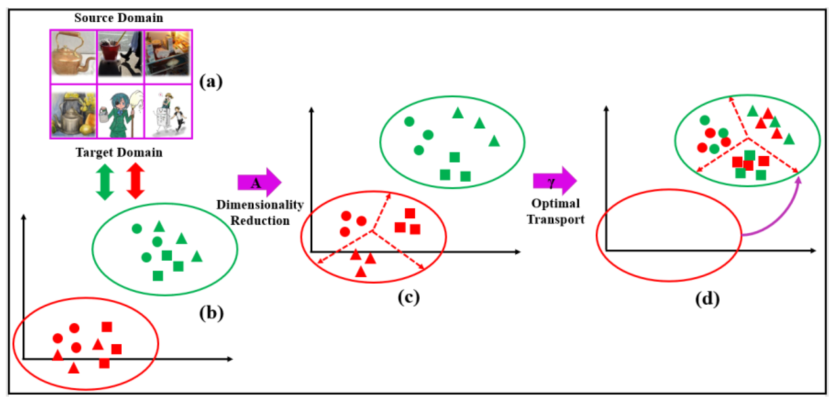
4.1. Motivation and Main Idea

The discriminability of the source data is essential for feature-based DA performance. The reviewed regularized OT methods for DA belonging to feature-based DA methods are based on OT-IT, which is efficient for high-dimensional cross-domain image classification. However, due to the entropy regularization, they usually lead to weak discriminability of the source data. Particularly, when $\lambda \to 0,$ ${\gamma }^{*}\left(i,j\right)=\frac{1}{n_s{n}_t},\forall i,j$ [27], it will cause all the source instances to be mapped to the same point in the target domain and the discriminability of the source domain will disappear unexpectedly.

To address this challenge, a two-stage procedure for feature-based adaptation is present in this paper. In the first stage, we construct a dimensionality reduction framework, similar to PCA, to learn a low-dimensional space while both the source and target data variation is maximized and the intraclass compactness in the source domain is minimized. In the second stage, based on the source and target low-dimensional features with the properties described in the first stage, we adopt class-based regularized optimal transport, i.e., Equation (3), to promote the interclass sparsity in the OTP rows (the OTP rows from different classes are sparse, so that the source instances from different classes are not associated with one same target instance) using the source label information.

Notably, the desirable properties in the first stage can mitigate the degradation of feature discriminability of the source domain in the second stage. Specifically, with the low-dimensionality space obtained in the first stage, the fluctuation range of all elements is getting larger in the cost matrix C, and the rows of C from the same classes tend to be similar. As such, the matrix C enables the OTP to have larger variance and enhances the intraclass density in rows of the OTP (that is, the OTP rows from the same classes are similar, so the source instances from the same classes are associated with one or more target instances simultaneously).

In this two-stage feature-based adaptation strategy, we can obtain an OTP with more discriminant information which can generate a more discriminative representation of the source domain when aligning the source features to the target features by minimizing the Wasserstein distance.

4.2. A Dimensionality Reduction Framework

OTDA usually reduces the source data variation, which may weaken the source interclass dispersion and degrade the discriminability of the source data. To address this challenge, we use dimensionality reduction to maximize the variation of both the source and target data and minimize the source intraclass compactness, which will lead to an OTP with larger variance and its rows from the same classes being intraclass denser when we conduct OT in the learned low-dimensional space.

Maximizing Intradomain Dispersion: Similar to principal component analysis (PCA), we propose to learn an orthogonal transformation matrix $A\in R^{d\times k}$ to separately maximize the variances of the $k$–dimensional embedded representations of the source and target domains. In order to ensure the existence of the orthogonal transformation matrix, a symmetric matrix is constructed to represent the variance, so that the orthogonal transformation matrix will be the solution of the following optimization problem:

$$\underset{A^{\mathrm{T}}A=I_k}{\max }\mathrm{tr}\left(A^{\mathrm{T}}\left(X_s^{\mathrm{T}}{H}_s{X}_s+X_t^{\mathrm{T}}{H}_t{X}_t\right)A\right),$$

(5)

where $M_1=X_s^{\mathrm{T}}{H}_s{X}_s+X_t^{\mathrm{T}}{H}_t{X}_t$ is the symmetric matrix, $H_s=I_{n_s}-\frac{1}{n_s}{1}_{n_s\times n_s}$ and $H_t=I_{n_t}-\frac{1}{n_t}{1}_{n_t\times n_t}$ are centering matrices, $I_p$ is an identity matrix, $p\in \left\{k,n_s,n_t\right\},$ and $1_{q\times q}$ is a $q\times q$ matrix whose elements are all ones, $q\in \left\{n_s,n_t\right\}$.

Minimizing the Source Intraclass Compactness: Intraclass compactness is a crucial indicator to measure the effectiveness of a model to produce discriminative features, where intraclass compactness indicates how close the features with the same label are to each other [37].

To retain the discriminative information of the source domain, minimization of the source intraclass compactness is added to the dimensionality reduction framework. The source intraclass compactness can be formulated as below:

$${\displaystyle \sum _{i=1}^{Cl}\frac{1}{n_s^{\left(i\right)}}}{\displaystyle \sum _{x_j^s,x_p^s\in {\mathsf{\Omega }}_s^{\left(i\right)}}{\Vert x_j^s-x_p^s\Vert }_2^2=}\mathrm{tr}\left(A^{\mathrm{T}}{X}_s^{\mathrm{T}}L{X}_{s}A\right),$$

(6)

where

$${\left(L\right)}_{j,p}=\{\begin{array}{cc}1,& j=p\\ -\frac{1}{n_s^{\left(i\right)}},& x_j^s,x_p^s\in {\mathsf{\Omega }}_s^{\left(i\right)}\\ 0,& otherwise\end{array}$$

(7)

is a symmetric matrix, and ${\mathsf{\Omega }}_s^{\left(i\right)}=\left\{x:x\in {\mathsf{\Omega }}_s\wedge y=i\right\},n_s^{\left(i\right)}=\left|{\mathsf{\Omega }}_s^{\left(i\right)}\right|$.

From Equation (6), we aim to minimize distance between each pair of data instances that come from the same class in the source domain, so that the source intraclass compactness is promoted. Notably, the weight $\frac{1}{n_s^{\left(i\right)}}$ is designed to pay more attention on the smaller-size class to deal with imbalance dataset problem.

According to the generalized Rayleigh quotient, the Equation (6), when minimized, can be integrated into Equation (5), and the feature reduction framework aims to find a transformation matrix by solving the following optimization problem:

$$\underset{A^{\mathrm{T}}\left(X_s^{\mathrm{T}}{H}_s{X}_s+X_t^T{H}_t{X}_t\right)A=I_k}{\min }\mathrm{tr}\left(A^T{X}_s^{T}L{X}_{s}A\right)+\beta {\Vert A\Vert }_F^2,$$

(8)

where $\beta$ is a trade-off parameter. Since $M_1=X_s^{\mathrm{T}}{H}_s{X}_s+X_t^{\mathrm{T}}{H}_t{X}_t$ and $M_2=X_s^{\mathrm{T}}L{X}_s$ are symmetric matrices, applying Lagrange techniques, the transformation matrix $A$ can be solved by finding the $k$–smallest eigenvectors corresponding to the following generalized eigen-decomposition:

$$\left(I_d+\beta X_s^{\mathrm{T}}L{X}_s\right)A=\left(X_s^T{H}_s{X}_s+X_t^{\mathrm{T}}{H}_t{X}_t\right)A\Phi ,$$

(9)

where $\Phi \in R^{k\times k}$ is a diagonal matrix with Lagrange multipliers.

Therefore, the low-dimensional features of the instances in both domains can be, respectively, represented as $Z_s=X_{s}A,Z_t=X_{t}A,$ where the intradomain samples are dispersed as much as possible and the source intraclass samples are compacted as much as possible.

4.3. OT Based on Low-Dimensional Representation

With the low-dimensional representation $Z_s={\left[z_1^s,z_2^s,\cdots ,z_{n_s}^s\right]}^{\mathrm{T}},Z_t={\left[z_1^t,z_2^t,\cdots ,z_{n_s}^t\right]}^{\mathrm{T}}$ learned above, we adopt OT-IT method to align the source and target features by transporting source data to the target domain at a minimum transport cost. As group-lasso regularized optimal transport (OT-GL) can further utilize the source label information by adding a $l_1-l_2$ class-based regularization to the OT-IT formulation to promote the interclass sparsity in the OTP rows, and also it can efficiently use the generalized conditional gradient (GCG) algorithm [38] to achieve better DA performance compared with other class-based regularized OT methods, we use OT-GL to obtain OTP and achieve the source and target feature alignment.

Based on the representation $Z_s={\left[z_1^s,z_2^s,\cdots ,z_{n_s}^s\right]}^{\mathrm{T}},Z_t={\left[z_1^t,z_2^t,\cdots ,z_{n_s}^t\right]}^{\mathrm{T}},$ the elements of the cost matrix can be computed by the squared $l_2$ Euclidean distance as follows:

$${\left(\overline{C}\right)}_{ij}={\Vert z_i-z_j\Vert }_2^2$$

(10)

Applying OT-GL, the OTP can be solved by the following formulation:

$${\gamma }^{*}=\underset{\gamma \in \mathsf{\Pi }}{\arg \min }{\langle \gamma ,\overline{C}\rangle }_F+\alpha {\displaystyle \sum _j{\displaystyle \sum _{Cl}{\Vert \gamma \left(L_{Cl},j\right)\Vert }_2}}+\frac{1}{\lambda }{\displaystyle \sum _{i,j}\gamma \left(i,j\right)\log }\gamma \left(i,j\right),$$

(11)

where $L_{Cl}=\left\{i:x_i^s\in \wedge y_i^s=Cl\right\}$. The GCG algorithm can efficiently solve the formulation to obtain the OTP. Since we adopt the above mentioned low-dimensional features and apply the class-based regularization, the resulting OTP can generate a more discriminative feature representation. Specifically, the OTP has larger variance and the rows of the OTP show greater intraclass density and interclass sparsity.

With the OTP, we can align the source and target features by mapping the source instances into the target domain to minimize the Wasserstein distance between their distributions and get a new representation of the source data as follows:

$${\tilde{Z}}_s=n_s{\gamma }^{*}{Z}_t.$$

(12)

In view of the above properties of the OTP, the new representation of the source data not only disperses the source interclass samples but also compacts the source intraclass samples, thus being more discriminative.

The proposed OTDR approach learns a low-dimensional feature representation to disperse the source/target instances and compact the source intraclass instances in the first stage. Then, with the desirable properties in the first stage, OT-GL method is adopted to map the source data instances into the target domain to achieve feature alignment in the second stage. Therefore, we can get a discriminative representation of the source data based on the OTP with interclass sparsity and intraclass density in its rows. In Algorithm 1, OTDR is summarized.

Algorithm 1: OTDR

Input: Data set $\left\{X_s,Y_s\right\},X_t;$ parameters $k,\beta ,\alpha ,\lambda .$

1: Construct a symmetric matrix $L$ using Equation (7).

2: Obtain the transformation matrix $A$ by calculating the $k$–smallest eigenvectors of Equation (9).

3: Let $Z_s=X_{s}A,Z_t=X_{t}A$, and compute the cost matrix $\overline{C}$ by Equation (10).

4: Adopt the GCG algorithm, and obtain the optimal transport plan ${\gamma }^{*}$ by solving Equation (11).

5: Generate ${\tilde{Z}}_s$ by Equation (12), and train an adaptive classifier $f$ on $\left\{{\tilde{Z}}_s,Y_s\right\}.$

Output: transformation matrix $A$, optimal transport plan ${\gamma }^{*}$, and adaptive classifier $f$.

5. Experiments

In this section, we conduct comprehensive experiments on cross-domain image classification datasets to validate the effectiveness of our approach.

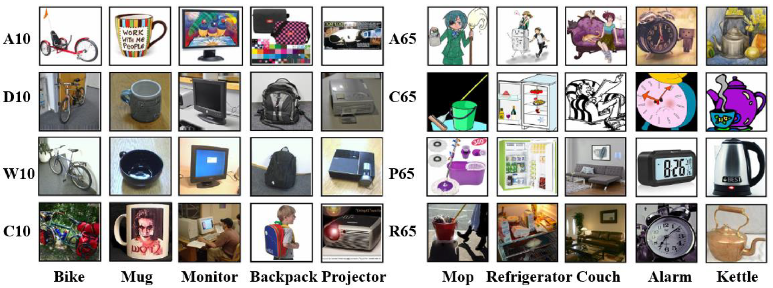
5.1. Data Descriptions

The widely used cross-domain datasets Office10 + Caltech10, ImageCLEF-DA, Office-31, and Office-Home were adopted in this paper in the form of A→B, which denotes a DA task from source domain A to target domain B. The statistics of these datasets are listed in

Table 1. Dataset descriptions.

Datasets	#Samples	#Classes	#Features	Domains
Office10 + Caltech10	2533	10	800/4096	A10, W10, D10, C10
Office-31	4652	31	2048	A31, W31, D31
ImageCLEF-DA	1800	12	2048	P12, T12, C12
Office-Home	15,500	65	2048	A65, C65, P65, R65

and some exemplary images from Office10 + Caltech10, Office-Home are shown in Figure 3.

Office10 + Caltech10 [7,39]: it has four domains, i.e., Amazon10 (A10), Webcam10 (W10), DSLR10 (D10), and Caltech10 (C10), in which 10 categories are shared. Accordingly, 12 DA tasks are established, i.e., A10→W10, A10→D10, etc. We utilize two feature sets, i.e., 800-dim SURF [16] and 4096-dim Decaf6 [40] features.

Office-31 [39]: it consists of 4652 images from three domains: Amazon (A31), Webcam (W31), and DSLR (D31), where 31 categories are shared. Likewise, six DA tasks are constructed, and we adopt 2048-dim ResNet-50 features learned from the ResNet-50 model [41].

ImageCLEF-DA (http://ai.bu.edu/visda-2017/): it includes 1800 images from three public domains: Pascal VOC 2012 (P12), ImageNet ILSVRC 2012 (I12), and Caltech-256 (C12), and there are 12 common categories. Similarly, we can create six DA tasks, and we also adopt the 2048-dim ResNet-50 features.

Office-Home [42]: it contains four domains, namely Art (A65), Clipart (C65), Product (P65), and Real World (R65), where 12 DA tasks could be constructed. There are more samples and categories in each domain, consequently, the DA tasks on this dataset are more challenging. Additionally, the ResNet-50 deep features are considered in our experiments.

5.2. Experimental Setting

We compare OTDR against various kinds of DA methods including OTDA methods (i.e., OT-IT [18], OT-GL [27], JDOT [35], KGOT [36]), other traditional DA methods (i.e., sample-to-sample correspondence (STSC) [22], GFK [14], subspace alignment (SA) [15], joint distribution adaptation (JDA) [17], transfer component analysis (TCA) [16], domain invariant and class discriminative feature learning (DICD) [24], joint geometrical and statistical alignment (JGSA) [29], adaptation regularization transfer learning (ARTL) [13], enhanced subspace distribution matching (ESDM) [43]), and several deep DA methods (i.e., deep adaptation network (DAN) [44], joint adaptation network (JAN) [20], domain adversarial neural network (DANN) [19], collaborative and adversarial network (CAN) [45], conditional domain adversarial network (CDAN) [46], the entropy conditioning variant of CDAN (CDAN + E) [46], domain-adversarial residual-transfer (DART) [47], multirepresentation adaptation network (MRAN) [48], transferable adversarial training (TAT) [49], learning explicitly transferable representations (LETR) [50], hybrid adversarial network (HAN) [51]).

For feature-based adaptation methods in all experiments, 1-NN classifier is used to predict the target labels. Since there are no labeled target instances, the optimal parameters of DA methods cannot be obtained by cross-validation steps. For the sake of fairness, we set the parameters of the comparison methods either to be the same as those recommended in the corresponding original papers or obtain them through empirical searching procedure for satisfactory DA performance. In our OTDR, like OT-GL algorithm, the group-lasso regularization, the entropy regularization parameters, and the maximum iterations in the GCG algorithm are set to $\alpha =2,\lambda =0.1$, $maxiter=20$. Besides, the reduced feature dimension is set to $k=200$. For the trade-off parameter in OTDR, according to the number of categories in different datasets, we set $\beta =0.001,0.01,0.1$ for Office-Home, Office-31, and Office10 + Caltech10/Image-CLEF-DA, respectively, which will be analyzed in the parameter sensitivity section.

5.3. Experimental Results

In this section, we adopted the classification accuracy to evaluate the effectiveness of proposed OTDR and the compared DA methods. As in [14,22,24,27,35,46], the metric of the classification accuracy is formulated as below $Accuracy=\frac{\left|x:x\in X_t\wedge f\left(x\right)=y\right|}{\left|x:x\in X_t\right|}$, where $y$ is the ground-truth label of $x$.

The classification accuracy of Office10 + Caltech10 (SURF features) and Office10 + Caltech10 (Decaf6 features) under different DA methods are shown in

Table 2. Accuracy (%) on Office 10 + Caltech 10 (SURF features).

Tasks	OT-IT	OT-GL	JDOT	KGOT	STSC	GFK	SA	TCA	JDA	DICD	ESDM	JGSA	OTDR
C10→A10	37.5	48.4	50.4	49.4	44.1	41.0	49.3	43.4	44.8	47.3	42.8	51.5	55.2
C10→W10	32.2	50.2	54.6	43.1	31.5	40.7	40.0	37.3	41.7	46.4	45.1	45.4	53.2
C10→D10	36.3	47.8	50.3	51.0	39.5	41.4	39.5	44.0	45.2	49.7	45.9	45.9	49.0
A10→C10	35.4	37.9	40.9	39.9	36.1	40.3	40.0	38.2	39.4	42.4	40.3	41.5	45.1
A10→W10	29.8	42.0	45.1	42.0	33.6	40.0	33.2	38.0	38.0	45.1	45.4	45.8	51.2
A10→D10	35.0	44.6	40.8	42.0	36.9	36.3	33.8	30.6	39.5	38.9	45.2	47.1	51.6
W10→C10	29.4	36.6	33.3	36.6	29.7	30.7	35.2	29.7	31.2	33.6	37.4	33.2	38.8
W10→A10	33.1	39.6	38.7	38.0	38.3	31.8	39.3	32.3	32.8	34.1	41.7	39.9	40.2
W10→D10	89.2	85.4	75.2	91.7	87.9	87.9	75.2	85.4	89.2	89.8	92.4	90.5	89.2
D10→C10	32.2	34.3	33.0	34.6	30.5	30.1	34.6	30.9	31.5	34.6	33.5	29.9	34.8
D10→A10	31.2	37.9	35.2	37.1	34.9	32.1	39.9	29.3	33.1	34.5	37.8	38.0	39.6
D10→W10	90.5	87.8	76.3	87.5	88.5	84.4	77.0	84.8	89.5	91.2	88.1	91.9	88.5
average	42.7	49.4	47.8	49.4	44.3	44.7	44.8	43.7	46.3	49.0	49.6	50.1	53.0

and

Table 3. Accuracy (%) on Office 10 + Caltech 10 (Decaf6 features).

Tasks	OT-IT	OT-GL	JDOT	KGOT	STSC	GFK	SA	TCA	JDA	DICD	JGSA	OTDR
C10→A10	88.7	92.1	91.5	91.4	89.9	88.2	89.4	90.2	90.3	91.0	91.4	93.0
C10→W10	75.2	84.2	88.8	87.1	81.2	77.6	81.4	77.0	85.1	92.2	86.8	91.2
C10→D10	83.4	87.3	89.8	92.4	87.5	86.6	90.5	85.4	89.2	93.6	93.6	89.8
A10→C10	81.7	85.5	85.2	85.7	85.6	79.2	80.6	82.7	84.0	86.0	84.9	87.0
A10→W10	78.9	83.1	84.8	82.4	81.4	70.9	83.1	74.6	78.6	81.4	81.0	88.8
A10→D10	85.9	85.0	87.9	86.6	87.1	82.2	89.2	80.3	80.9	83.4	88.5	87.3
W10→C10	74.8	81.5	82.6	85.0	81.6	69.7	79.8	79.9	84.2	84.0	85.0	85.0
W10→A10	81.0	90.6	90.7	89.7	88.9	76.8	83.8	84.5	90.1	89.7	90.7	92.5
W10→D10	95.6	96.3	98.1	100.0	99.0	100.0	100.0	100.0	100.0	100.0	100.0	100.0
D10→C10	77.7	84.1	84.3	85.6	83.7	71.4	81.4	82.5	85.0	86.1	86.2	86.4
D10→A10	87.2	92.3	88.1	91.8	92.7	76.3	87.1	88.2	91.0	92.2	92.0	92.4
D10→W10	93.8	96.3	96.6	99.3	96.1	99.3	99.3	99.7	100.0	99.0	99.7	99.3
average	83.7	88.5	89.2	89.8	87.9	81.5	87.1	85.4	88.2	89.9	90.0	91.1

, where we can observe that OTDR outperforms all of the feature-based adaptation methods with an average classification accuracy of 53%.

JGSA combines subspace alignment and distribution alignment to reduce the cross-domain divergence, which is better than the pure subspace alignment methods, i.e., GFK, SA, and the pure distribution alignment methods, i.e., TCA, JDA, DICD, ESDM.

Although, those seven methods achieve DA by global feature alignment, they ignore the local information. STSC and OTDA methods, i.e., OT-IT, OT-GL, KGOT, JDOT utilize sample-to-sample matching to exploit the local information, while they do not further explore the source label information. As such, the DA performance of these methods is degraded and they cannot beat JGSA on average.

Based on OT-GL, our OTDR further uses the source label information and a two-stage feature-based adaptation strategy to alleviate the source discriminability degradation caused by OT-GL. Therefore, OTDR stands out among these sample-to-sample matching methods on most of the tasks (17/24 tasks). Moreover, compared with the best baseline JGSA, our OTDR has 3.0% improvements.

To further evaluate the performance of OTDR, we conducted experiments on three datasets with ResNet-50 features. The results of OT-GL, the best baseline feature-based DA method, i.e., JGSA, the state-of-the-art classifier-based DA method, i.e., ARTL, and several end-to-end deep DA models are reported in

Table 4. Accuracy (%) on Office-31 and ImageCLEF-DA.

Tasks	OT-GL	JGSA	ARTL	DAN	DANN	JAN	CAN	DART	MRAN	OTDR
A31→W31	81.3	86.5	85.0	80.5	82.0	85.4	81.5	87.3	91.4	88.4
D31→W31	93.7	98.4	94.2	97.1	96.9	97.4	98.2	98.4	96.9	96.5
W31→D31	96.0	99.8	97.2	99.6	99.1	99.8	99.7	99.9	99.8	98.6
A31→D31	86.8	90.0	82.5	78.6	79.7	84.7	85.5	91.6	86.4	91.2
D31→A31	66.6	71.1	71.0	63.6	68.2	68.6	65.9	70.3	68.3	71.1
W31→A31	67.7	71.4	70.7	62.8	67.4	70.0	63.4	69.7	70.9	72.1
I12→P12	78.3	77.5	71.3	74.5	66.5	76.8	78.2	78.3	78.8	79.5
P12→I12	89.0	86.7	84.2	82.2	81.8	88.0	87.5	89.3	91.7	91.0
I12→C12	96.0	95.0	87.2	92.8	89.0	94.7	94.2	95.3	95.0	97.2
C12→I12	93.3	93.2	84.7	86.3	79.8	89.5	89.5	91.0	93.5	93.5
C12→P12	77.7	76.8	70.3	69.2	63.5	74.2	75.8	75.2	77.7	78.8
P12→C12	92.5	88.3	87.2	89.8	88.7	93.5	89.2	93.1	95.3	95.3
average	85.0	86.2	82.1	81.4	80.2	85.2	84.1	86.6	87.1	87.8

and

Table 5. Accuracy (%) on Office-Home.

Tasks	OT-GL	JGSA	ARTL	DAN	DANN	JAN	CDAN	CDAN + E	TAT	LETR	HAN	OTDR
A65→C65	45.9	48.6	53.9	43.6	45.6	45.9	49.0	50.7	51.6	52.0	52.0	55.9
A65→P65	68.2	71.6	75.0	57.0	59.3	61.2	69.3	70.6	69.5	72.6	72.0	75.9
A65→R65	71.5	76.1	75.6	67.9	70.1	68.9	74.5	76.0	75.4	78.2	75.8	80.5
C65→A65	52.6	48.7	53.4	45.8	47.0	50.4	54.4	57.6	59.4	58.2	59.6	58.8
C65→P65	65.2	68.4	72.4	56.5	58.5	59.7	66.0	70.0	69.5	69.8	71.8	73.6
C65→R65	65.5	67.5	70.6	60.4	60.9	61.0	68.4	70.0	68.6	70.3	71.2	72.0
P65→A65	54.8	53.8	56.2	44.0	46.1	45.8	55.6	57.4	59.5	62.9	58.7	58.2
P65→C65	46.6	44.2	51.4	43.6	43.7	43.4	48.3	50.9	50.5	47.8	51.3	51.3
P65→R65	74.4	76.7	76.1	67.7	68.5	70.3	75.9	77.3	76.8	78.1	77.7	78.1
R65→A65	62.5	61.7	65.3	63.1	63.2	63.9	68.4	70.9	70.9	70.6	72.8	65.5
R65→C65	50.8	51.9	56.7	51.5	51.8	52.4	55.4	56.7	56.6	55.3	57.7	55.9
R65→P65	77.5	78.7	81.0	74.3	76.8	76.8	80.5	81.6	81.6	82.5	82.3	82.9
average	61.3	62.3	65.6	56.3	57.6	58.3	63.8	65.8	65.8	66.5	66.9	67.4

.

It can be seen that the traditional DA methods are superior to some deep DA methods, i.e., DAN, DANN, JAN on average. In this sense, the research of traditional DA method is still meaningful.

In addition, OTDR also outperforms OT-GL, JGSA, and ARTL based on ResNet-50 features on most of the tasks (19/24 tasks), which further indicates that OTDR is significant in traditional methods. More importantly, OTDR is on average better than all of the baseline deep DA methods on average.

In particular, for the challenging large Office-Home dataset, OTDR has 0.5% improvements against the best baseline HAN. Hence, the results indicate that OTDR can achieve DA marginally on cross-domain image classification tasks compared with either traditional or deep DA methods.

6. Discussion

6.1. Distribution of the OPT Matrix

To verify the effectiveness of proposed OTDR, we first inspected the distribution of the OTP matrix on randomly selected task C10→A10 with SURF features as shown in Figure 4.

It can be seen from Figure 4a that the OTP ${\gamma }^{*}$ obtained by OT-IT is smoothest as a whole without source label information, which will result in a source feature representation with relatively poor discriminability.

When the class-based regularization is added to OT-IT, the interclass sparsity in the OTP rows can be enhanced as shown in Figure 4b, where the 10 small matrix blocks on the diagonal represent the transport plan between the source and target samples from the same class, respectively. However, there are some wrong transport directions in this OTP, i.e., some source instances of the same class are transported to target instances of different classes.

To enhance the discriminability of the source data, our OTDR approach performs dimensionality reduction procedure before OT. In this way, compared with OT-GL, the obtained OTP has more elements with a variance of 1.3 × 10⁻⁶ (while the variance of the OTP obtained by adopting OT-GL is $9.1\times {10}^{-7}$). Furthermore, the OTP shows higher intraclass density in its rows, as is shown in Figure 4c, which prompts all of the source samples from the same classes to be associated with one or more target instances simultaneously. Therefore, the OPT will generate more a discriminative representation of the source domain.

6.2. Statistics of Feature Discriminability

In addition, we evaluated the discriminability of the feature representation of the transported source instances on five randomly selected DA tasks (i.e., C10→A10 with SURF features, W10→C10 with Decaf6 features, W31→A31, P12→C12, C65→R65) by showing the ratio of the source intradomain dispersion (“S_dispersion”) to the target intradomain dispersion (“T_dispersion”) and the ratio of the source intraclass compactness (“S_compactness”) to the source intradomain dispersion (“S_dispersion”) in Figure 5.

As can be seen from Figure 5a, the “S_dispersion/T_dispersion” under OT-GL is sharply reduced, that is, the source instances are crowded relative to the target instances, which may lead to weaker discriminability of the source domain. It corresponds to our motivation.

Using OTDR, we can obtain an OTP, which shows more obvious interclass sparsity and intraclass density in its rows, thus a more discriminative representation of the source data can be generated. The discriminability can be indicated by trends of the “S_compactness/S_dispersion”, as shown in Figure 5b, where we can see that compared with OT-GL, “S_compactness/S_dispersion” under OTDR is smaller.

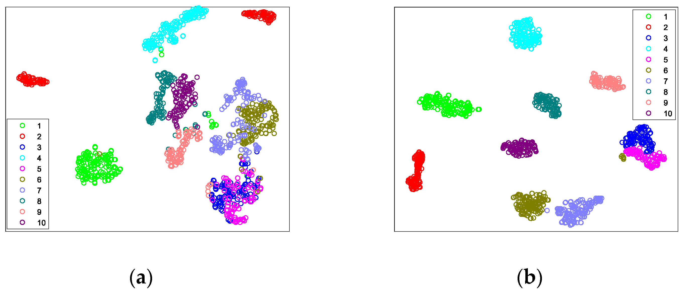
6.3. Feature Visualization of Source Domain

Moreover, by displaying the t-SNE feature visualization [40] of task C10→A10 with SURF features in Figure 6, the discriminability of the source data can be illustrated intuitively and the features used in Figure 6a,b are generated by OT-GL and OTDR, respectively.

We observe that the source instances under OT-GL from different classes cluster together, which is consistent with our speculation mentioned above, while the source instances under OTDR are more discriminative.

6.4. Ablation Study

Finally, we conducted experiments on the five DA tasks used above to verify the effectiveness of the intraclass compactness minimization and the intradomain dispersion maximization.

As shown in Figure 7, by removing the intraclass compactness regularization (OTDR/ICR), the classification accuracy is reduced on all the five tasks compared with OTDR. In addition, when we further remove the intradomain dispersion maximization, that is, drop the dimensionality reduction procedure, OTDR degenerates to OT-GL and the classification accuracy is further reduced as shown in Figure 7. Therefore, in DA process, it is effective to minimize the intraclass compactness and maximize the intradomain dispersion.

6.5. Parameter Sensitivity

Since $\alpha =2,\lambda =0.1,maxiter=20$ are fixed to be the same as OT-GL on all DA tasks, we only evaluate the sensitivity of the reduced feature dimensions $k$ and the trade-off parameter $\beta$ on the five DA tasks used above by fixing one parameter to analyze the other. Specifically, we set $k\in \left\{20,40,60,\cdots ,400\right\}$ and $\beta \in \left\{{10}^{-5},\frac{{10}^{-4}}{2}{,10}^{-4},\frac{{10}^{-3}}{2},\cdots ,\frac{{10}^2}{2},{10}^2\right\}$, respectively. The classification accuracy curves under our OTDR are presented in Figure 8 and the trends on all other tasks are similar. From Figure 8a, we observe that as the value of $k$ increases, the accuracy results are higher and then tend to be stabilize within the range of $k\in \left\{80,100,\cdots ,400\right\}$. Therefore, we can choose parameter $k$ in a wide range to obtain optimal performance.

For the trade-off parameter $\beta$, small values of $\beta$ can make the source intraclass compactness minimization more effective, and an infinite value of $\beta$ will cause the source intraclass compactness effectiveness to be ignored. As the value increases inside the range $\beta \in \left\{{10}^{-3}{,10}^{-2},\cdots ,{10}^2\right\}$, the accuracy results shown in Figure 8b also increase, reaching the top performance, then decrease slightly and then tend to stabilize, so that OTDR can achieve good performance in a relatively wider range of $\beta$. Specifically, the top performance of OTDR can be achieved in $\beta \in \left[5{\ast 10}^{-3},{10}^0\right]$ and $\beta \in \left[{10}^{-4},{10}^{-1}\right]$ for few-category datasets (i.e., Office10 + Caltech10, Image-CLEF-DA) and multicategory datasets (i.e., Office-31, Office-Home), respectively.

7. Conclusions

In this paper, a novel two-stage feature-based adaptation approach for domain adaptation (DA) referred to as optimal transport with dimensionality reduction (OTDR) was proposed to promote DA performance. We attempted to enhance the discriminability of the source domain when aligning the source and target features. OTDR uses source label information in two stages to obtain an OTP with larger variance so as to promote the interclass sparsity and intraclass density in its rows, which can generate a more discriminative feature representation of the source domain when aligning the source features to the target features by minimizing the Wasserstein distance between source and target distributions. Comprehensive experiments conducted on different DA tasks demonstrate that OTDR is competitive with traditional and deep DA baselines.

8. Future Work

OTDR achieves feature adaptation in two separate stages for DA, i.e., low-dimensionality learning, optimal transport, while in the first stage, some original information might be distorted. In future work, we will consider embedding the preservation of the source data discriminability and the optimal transport from source data to target data into deep architectures for end-to-end deep domain adaptation.

References

1. Paszkiel, S. Using Neural Networks for Classification of the Changes in the EEG Signal Based on Facial Expressions. In Analysis and Classification of EEG Signals for Brain—Computer Interfaces; Kacprzyk, J., Ed.; Springer: Cham, Switzerland, 2020; Volume 852, pp. 41–69. [Google Scholar]
2. Paszkiel, S. The use of facial expressions identified from the level of the EEG signal for controlling a mobile vehicle based on a state machine. In Proceedings of the Conference on Automation, Warsaw, Poland, 18–20 March 2020; pp. 227–238. [Google Scholar]
3. Paszkiel, S.; Dobrakowski, P.; Łysiak, A. The impact of different sounds on stress level in the context of EEG, Cardiac Measures and Subjective Stress Level: A Pilot Study. Brain Sci. 2020, 10, 728. [Google Scholar] [CrossRef] [PubMed]
4. Paszkiel, S.; Sikora, M. The use of brain-computer interface to control unmanned aerial vehicle. In Proceedings of the Conference on Automation, Warsaw, Poland, 27–29 March 2019; pp. 583–598. [Google Scholar]
5. Gopalan, A.B.; Li, R.; Chellappa, R. Domain adaptation for object recognition: An unsupervised approach. In Proceedings of the IEEE International Conference on Computer Vision, Barcelona, Spain, 6–13 November 2011; pp. 999–1006. [Google Scholar]
6. Zhang, L.; Yang, J.; Zhang, D. Domain class consistency based transfer learning for image classification across domains. Inf. Sci. 2017, 418, 242–257. [Google Scholar] [CrossRef]
7. Griffin, G.; Holub, A.; Perona, P. Caltech-256 Object Category Dataset, Technical Report 7694 Caltech. 2007. Available online: http://www.vision.caltech.edu/archive.html (accessed on 15 November 2006).
8. Pan, S.J.; Yang, Q. A survey on transfer learning. IEEE Trans. Knowl. Data Eng. 2010, 22, 1345–1359. [Google Scholar] [CrossRef]
9. Dai, Y.; Zhang, J.; Yuan, S.; Xu, Z. A two-stage multi-task learning-based method for selective unsupervised domain adaptation. In Proceedings of the International Conference on Data Mining Workshops, Beijing, China, 8–11 November 2019; pp. 863–868. [Google Scholar]
10. Dai, W.; Yang, Q.; Xue, G.R.; Yu, Y. Boosting for transfer learning. In Proceedings of the 24th International Conference on Machine Learning, Corvallis, OR, USA, 20–24 June 2007; pp. 193–200. [Google Scholar]
11. Huang, J.; Gretton, A.; Borgwardt, K.; Schölkopf, B.; Smola, A.J. Correcting sample selection bias by unlabeled data. In Advances in Neural Information Processing Systems, Proceedings of the Advances in Neural Information Processing Systems 19, Proceedings of the Twentieth Annual Conference on Neural Information Processing Systems, Vancouver, BC, Canada, 3–6 December 2007; MIT Press: Cambridge, MA, USA, 2007; pp. 601–608. [Google Scholar]
12. Tao, J.; Chung, F.L.; Wang, S. On minimum distribution discrepancy support vector machine for domain adaptation. Pattern Recognit. 2012, 45, 3962–3984. [Google Scholar] [CrossRef]
13. Long, M.; Wang, J.; Ding, G.; Pan, S.J.; Philip, S.Y. Adaptation regularization: A general framework for transfer learning. IEEE Trans. Knowl. Data Eng. 2014, 26, 1076–1089. [Google Scholar] [CrossRef]
14. Gong, B.; Shi, Y.; Sha, F.; Grauman, K. Geodesic flow kernel for unsupervised domain adaptation. In Proceedings of the IEEE Conference on Computer Vision and Pattern Recognition, Providence, RI, USA, 16–21 June 2012; pp. 2066–2073. [Google Scholar]
15. Fernando, B.; Habrard, A.; Sebban, M.; Tuytelaars, T. Unsupervised visual domain adaptation using subspace alignment. In Proceedings of the IEEE International Conference on Computer Vision, Sydney, Australia, 1–8 December 2013; pp. 2960–2967. [Google Scholar]
16. Pan, S.J.; Tsang, I.W.; Kwok, J.T.; Yang, Q. Domain adaptation via transfer component analysis. IEEE Trans. Neural Netw. 2011, 22, 199–210. [Google Scholar] [CrossRef] [Green Version]
17. Long, M.; Wang, J.; Ding, G.; Sun, J.; Yu, P.S. Transfer feature learning with joint distribution adaptation. In Proceedings of the IEEE International Conference on Computer Vision, Portland, OR, USA, 23–28 June 2013; pp. 2200–2207. [Google Scholar]
18. Courty, N.; Flamary, R.; Tuia, D. Domain adaptation with regularized optimal transport. In Proceedings of the European Conference on Machine Learning and Principles and Practice of Knowledge Discovery in Databases, Nancy, France, 15–19 September 2014; pp. 274–289. [Google Scholar]
19. Ganin, Y.; Ustinova, E.; Ajakan, H.; Germain, P.; Larochelle, H.; Laviolette, F.; Marchand, M.; Lempitsky, V. Domain-adversarial training of neural networks. J. Mach. Learn. Res. 2016, 17, 1–35. [Google Scholar]
20. Long, M.; Zhu, H.; Wang, J.; Jordan, M.I. Deep transfer learning with joint adaptation networks. In Proceedings of the Conference on Machine Learning, Sydney, Australia, 6–11 August 2017; pp. 2208–2217. [Google Scholar]
21. Wang, M.; Deng, W. Deep visual domain adaptation: A survey. Neurocomputing 2018, 312, 135–153. [Google Scholar] [CrossRef] [Green Version]
22. Das, D.; Lee, C.S.G. Sample-to-sample correspondence for unsupervised domain adaptation. Eng. Appl. Artif. Intell. 2018, 73, 80–91. [Google Scholar] [CrossRef] [Green Version]
23. Tahmoresnezhad, J.; Hashemi, S. Visual domain adaptation via transfer feature learning. Knowl. Inf. Syst. 2017, 50, 585–605. [Google Scholar] [CrossRef]
24. Li, S.; Song, S.; Huang, G.; Ding, Z.; Wu, C. Domain invariant and class discriminative feature learning for visual domain adaptation. IEEE Trans. Image Process. 2018, 27, 4260–4273. [Google Scholar] [CrossRef] [PubMed]
25. Baktashmotlagh, M.; Harandi, M.T.; Lovell, B.C.; Salzmann, M. Unsupervised domain adaptation by domain invariant projection. In Proceedings of the IEEE International Conference on Computer Vision, Portland, OR, USA, 23–28 June 2013; pp. 769–776. [Google Scholar]
26. Sun, B.; Feng, J.; Saenko, K. Return of frustratingly easy domain adaptation. In Proceedings of the AAAI Conference on Artificial Intelligence, Phoenix, AZ, USA, 12–17 February 2016; pp. 2058–2065. [Google Scholar]
27. Courty, N.; Flamary, R.; Tuia, D.; Rakotomamonjy, A. Optimal transport for domain adaptation. IEEE Trans. Pattern Anal. Mach. Intell. 2017, 39, 1853–1865. [Google Scholar] [CrossRef] [PubMed]
28. Kantorovich, L. On the translocation of masses. Manag. Sci. 1958, 5, 1–142. [Google Scholar] [CrossRef]
29. Zhang, J.; Li, W.; Ogunbona, P. Joint geometrical and statistical alignment for visual domain adaptation. In Proceedings of the IEEE Conference on Computer Vision and Pattern Recognition, San Juan, PR, USA, 24–30 June 2017; pp. 5150–5158. [Google Scholar]
30. Li, J.; Jing, M.; Lu, K.; Shen, H.T. Locality preserving joint transfer for domain adaptation. IEEE Trans. Image Process. 2019, 28, 6103–6115. [Google Scholar] [CrossRef] [Green Version]
31. Li, J.; Lu, K.; Huang, Z.; Zhu, L.; Shen, H. Transfer independently together: A generalized framework for domain adaptation. IEEE Trans. Cybern. 2019, 49, 2144–2155. [Google Scholar] [CrossRef]
32. Ferradans, S.; Papadakis, N.; Peyré, G.; Aujol, J. Regularized discrete optimal transport. SIAM J. Imaging Sci. 2013, 7, 428–439. [Google Scholar]
33. Rabin, J.; Ferradans, S.; Papadakis, N. Adaptive color transfer with relaxed optimal transport. In Proceedings of the IEEE International Conference on Image Processing, Columbus, OH, USA, 24–27 June 2014; pp. 4852–4856. [Google Scholar]
34. Cuturi, M. Sinkhorn distances: Lightspeed computation of optimal transport. In Proceedings of the Advances in Neural Information Processing Systems, Lake Tahoe, NV, USA, 5–10 December 2013; pp. 2292–2300. [Google Scholar]
35. Courty, N.; Flamary, R.; Habrard, A.; Rakotomamonjy, A. Joint distribution optimal transportation for domain adaptation. In Advances in Neural Information Processing Systems, Proceedings of the 31st International Conference on Neural Information Processing Systems, Long Beach, CA, USA, 4–9 December 2017; MIT Press: Cambridge, MA, USA, 2017; pp. 3733–3742. [Google Scholar]
36. Zhang, Z.; Wang, M.; Nehorai, A. Optimal transport in reproducing kernel Hilbert spaces: Theory and applications. IEEE Trans. Pattern Anal. Mach. Intell. 2020, 42, 1741–1754. [Google Scholar] [CrossRef] [Green Version]
37. Luo, Y.; Wong, Y.; Kankanhalli, M.; Zhao, Q. G-Softmax: Improving intraclass compactness and interclass separability of features. IEEE Trans. Neural Netw. Learn. Syst. 2019, 31, 685–699. [Google Scholar] [CrossRef]
38. Bredies, K.; Lorenz, D.A.; Maass, P. A generalized conditional gradient method and its connection to an iterative shrinkage method. Comput. Optim. Appl. 2009, 42, 173–193. [Google Scholar] [CrossRef]
39. Saenko, K.; Kulis, B.; Fritz, M.; Darrell, T. Adapting visual category models to new domains. In Proceedings of the European Conference on Computer Vision, Heraklion, Crete, Greece, 5–11 September 2010. [Google Scholar]
40. Donahue, J.; Jia, Y.; Vinyals, O.; Hoffman, J.; Zhang, N.; Tzeng, E.; Darrell, T. Decaf: A deep convolutional activation feature for generic visual recognition. In Proceedings of the International Conference on Machine Learning, Beijing, China, 22–24 June 2014; pp. 647–655. [Google Scholar]
41. He, K.; Zhang, X.; Ren, S.; Sun, J. Deep residual learning for image recognition. In Proceedings of the IEEE Conference on Computer Vision and Pattern Recognition, Las Vegas, NV, USA, 26 June–1 July 2016; pp. 770–778. [Google Scholar]
42. Venkateswara, H.; Eusebio, J.; Chakraborty, S.; Panchanathan, S. Deep hashing network for unsupervised domain adaptation. In Proceedings of the IEEE Conference on Computer Vision and Pattern Recognition, San Juan, PR, USA, 24–30 June 2017; pp. 5385–5394. [Google Scholar]
43. Kang, Q.; Yao, S.; Zhou, M.C.; Zhang, K.; Abusorrah, A. Enhanced subspace distribution matching for fast visual domain adaptation. IEEE Trans. Comput. Soc. Syst. 2020, 7, 1047–1057. [Google Scholar] [CrossRef]
44. Long, M.; Cao, Y.; Wang, J.; Jordan, M. Learning transferable features with deep adaptation networks. In Proceedings of the International Conference on Machine Learning, Lille, France, 7–9 July 2015; pp. 97–105. [Google Scholar]
45. Zhang, W.; Ouyang, W.; Li, W.; Xu, D. Collaborative and adversarial network for unsupervised domain adaptation. In Proceedings of the IEEE Conference on Computer Vision and Pattern Recognition, Salt Lake City, UT, USA, 18–22 June 2018; pp. 3801–3809. [Google Scholar]
46. Long, M.; Cao, Z.; Wang, J.; Jordan, M.I. Conditional adversarial domain adaptation. In Advances in Neural Information Processing Systems, Proceeding of the 32nd Conference on Neural Information Processing Systems (NeurIPS 2018), Montréal, QC, Canada, 2–8 December 2018; MIT Press: Cambridge, MA, USA, 2018; pp. 1647–1657. [Google Scholar]
47. Fang, X.; Bai, H.; Guo, Z.; Shen, B.; Hoi, S.; Xu, Z. DART: Domain-adversarial residual-transfer networks for unsupervised cross-domain image classification. Neural Netw. 2020, 127, 182–192. [Google Scholar] [CrossRef] [PubMed] [Green Version]
48. Zhu, Y.; Zhuang, F.; Wang, J.; Chen, J.; Shi, Z.; Wu, W.; He, Q. Multi-representation adaptation network for cross-domain image classification. Neural Netw. 2019, 119, 214–221. [Google Scholar] [CrossRef] [PubMed]
49. Liu, H.; Long, M.; Wang, J.; Jordan, M.I. Transferable adversarial training: A general approach to adapting deep classifiers. In Proceedings of the International Conference on Machine Learning, Berkeley, CA, USA, 9–15 June 2019; pp. 4013–4022. [Google Scholar]
50. Jing, M.; Li, J.; Lu, K.; Zhu, L.; Yang, Y. Learning explicitly transferable representations for domain adaptation. Neural Netw. 2020, 130, 39–48. [Google Scholar] [CrossRef] [PubMed]
51. Zhang, C.; Zhao, Q.; Wang, Y. Hybrid adversarial network for unsupervised domain adaptation. Inf. Sci. 2020, 514, 44–55. [Google Scholar] [CrossRef]
Figure 1. Translation learning between different languages without enough corpus; image recognition between different domains sampled from different visual angles, backgrounds, illustrations; activity recognition for different users, devices, locations; document translation and sentiment analysis between different domains, backgrounds; man–machine interactive for different users, interfaces, situations; indoor location with different scenarios, devices, moments.
Symmetry 12 01994 g001
Figure 2. (a) Exemplary images from the source and target domains; (b) traditional or deep features of source and target domains; (c) first stage: dimensionality reduction to promote source intraclass compactness, and improve source and target intradomain dispersion; (d) second stage: optimal transport to align the source and target distributions with desirable properties obtained in the first stage.
Symmetry 12 01994 g002
Figure 3. Exemplary images from Office10 + Caltech10 (left part, four domains), Office-Home (right part, four domains).
Symmetry 12 01994 g003
Figure 4. (a) γ * for task C10→A10 under information theoretic regularized optimal transport (OT-IT); (b) γ * for task C10→A10 under group-lasso regularized optimal transport (OT-GL); (c) γ * for task C10→A 10 under optimal transport with dimensionality reduction (OTDR).
Symmetry 12 01994 g004
Figure 5. (a) S_dispersion/T_dispersion under Original, OT_GL, and OTDR; (b) S_compactness/S_dispersion under OT_GL and OTDR.
Symmetry 12 01994 g005
Figure 6. (a) Feature visualization of the task C10→A10 under OT_GL; (b) feature visualization of the task C10→A10 under OTDR. Various colors denote different categories, the hollow dots are the feature of source data instances that are projected into a 2-dimensional using t-SNE feature visualization.
Symmetry 12 01994 g006
Figure 7. Classification accuracy of OT-GL, OTDR by removing the intraclass compactness regularization (OTDR/ICR), OTDR.
Symmetry 12 01994 g007
Figure 8. Parameter sensitivity of OTDR: (a) dimensions k ; (b) trade-off parameter β .
Symmetry 12 01994 g008