Article

An fMRI Feature Selection Method Based on a Minimum Spanning Tree for Identifying Patients with Autism

School of Artificial Intelligence, Beijing Normal University, Beijing 100875, China
*
Author to whom correspondence should be addressed.
Symmetry 2020, 12(12), 1995; https://doi.org/10.3390/sym12121995
Submission received: 9 November 2020 / Revised: 25 November 2020 / Accepted: 2 December 2020 / Published: 3 December 2020
(This article belongs to the Section Computer)

Abstract

:
Autism spectrum disorder (ASD) is a neurodevelopmental disorder originating in infancy and childhood that may cause language barriers and social difficulties. However, in the diagnosis of ASD, the current machine learning methods still face many challenges in determining the location of biomarkers. Here, we proposed a novel feature selection method based on the minimum spanning tree (MST) to seek neuromarkers for ASD. First, we constructed an undirected graph with nodes of candidate features. At the same time, a weight calculation method considering both feature redundancy and discriminant ability was introduced. Second, we utilized the Prim algorithm to construct the MST from the initial graph structure. Third, the sum of the edge weights of all connected nodes was sorted for each node in the MST. Then, N features corresponding to the nodes with the first N smallest sum were selected as classification features. Finally, the support vector machine (SVM) algorithm was used to evaluate the discriminant performance of the aforementioned feature selection method. Comparative experiments results show that our proposed method has improved the ASD classification performance, i.e., the accuracy, sensitivity, and specificity were 86.7%, 87.5%, and 85.7%, respectively.

1. Introduction

Autism spectrum disorder (ASD) is a group of neurodevelopmental deficits. According to recent research reports, one in every 45 children suffers from ASD, which may cause significant social, communication and behavioral challenges [1,2,3,4,5,6]. In terms of the etiology and diagnosis of ASD, ASD is a widespread developmental disorder caused by diseases of the brain and nervous system, as well as gene mutations [7]. In general, some symptoms of ASD begin to appear gradually at approximately two years of age [8]. A noninvasive method for diagnosing ASD in the early stage may help clinicians implement interventions in a timely manner and significantly improve patients′ quality of life [9,10]. In recent decades, various noninvasive brain imaging methods have been widely used in ASD studies, such as electroencephalography [11], structural magnetic resonance imaging [12], resting-state magnetic resonance imaging [13,14], and diffusion tensor imaging [15], and these methods have made outstanding contributions to extracting biomarkers that characterize disease characteristics. Recently, machine learning has been used in the field of neuroimaging, because it accurately and automatically distinguishes individuals with schizophrenia from healthy people [16,17]. In light of the ASD auxiliary diagnosis, machine learning is often utilized in three key steps: (1) constructing functional connectivity networks among regions of interest (ROIs) from resting state functional magnetic resonance imaging (rs-fMRI) data, (2) analyzing the connectivity of brain regions and identifying differences in connectivity between patients and normal controls, and (3) building a classification model to discriminate individuals with ASD from non-ASD subjects using filtered functional connectivity features [18]. Here, the functional connections are always represented by Pearson′s correlation coefficient matrix. However, the high dimensionality of the functional connection matrix usually reduces the classification performance, particularly under the condition of a lack of sufficient neural image samples. The influx of features into classifiers is known as dimensional disasters and overfitting. Thus, the selection of fMRI features is particularly important in disease classification and prediction [19].
To the best of our knowledge, research on feature selection algorithms based on ASD diagnosis in the existing literature has mainly covered two methods. One feature selection method is a filter-based method. The filter method first selects the features of the dataset and then trains the classifier with the feature subset. Notably, the process of feature selection and the subsequent classification are performed independently. For example, Guo [20] designed a two-sample t-test method to classify patients with ASD, and the accuracy rate was 70.67%. However, the t-test method is mainly applied to the usage scenarios of small sample data. The identification method of the statistical test relies on the difference between groups and obtains the optimal feature subset based on the p-value [21,22,23,24,25]. Mladen et al. [26] introduced the Fisher score [27] to identify patients with ASD according to the features of the same feature data distribution. The method analyzed MRI information from two dimensions of function and structure, which can obtain stronger information expression ability and the classification accuracy reached 85.06%. Kang et al. [28] combined the minimum redundancy maximum correlation (mRMR) feature selection method with the SVM classifier to classify children with autism and typical children, and the resulting classification accuracy was 85.44%. Nevertheless, the mRMR algorithm may underestimate the effectiveness of features to a certain extent. The other feature selection method is based on wrapping and embedding. Specifically, the wrapping method directly utilizes the performance of the final classifier to evaluate the total effects of feature selection and classification, while the embedded method combines the feature selection process with the classifier training process, i.e., the feature is automatically selected during the classifier training process. For instance, Fredo et al. [29] classified functional magnetic resonance images (fMRI) of typically developing (TD) individuals and participants with ASD using a conditional random forest model. The dimensionality of the functional connectivity (FC) matrix was reduced using conditional random forest models, and the classification accuracy was 65%. Taban et al. [30] adopted an autoencoder and a single-layer perceptron to diagnose ASD and achieved an accuracy of 70.3%. To overcome the shortcomings of poor generalization ability in single-layer neural network and obtain the multi-granularity information hidden in fMRI data. Li et al. [31] proposed a patch-level data-expanding strategy for multi-channel convolutional neural networks to automatically identify infants with risk of ASD in early age and the accuracy rate reached 76.24%. The various statistical methods, machine learning methods, and deep learning methods described above all promote research into the diagnosis of ASD.
The current feature selection methods are not good at facilitating the diagnosis of ASD. Due to the high-dimensional characteristics of fMRI data, mutually exclusive information or redundant information between features may be included. Traditional filter-based or wrapper-based methods always tend to select features containing discrimination information and do not closely monitor the information redundancy among features at the same time. From the perspective of feature selection, the model we construct must have both the ability to select discriminative features and filter out redundant information. The current feature selection methods aim to minimize the redundancy between features based on the identification of features that maximize the class difference without fully considering the decoupling of fMRI features. We proposed a feature selection method based on the minimum spanning tree (MST) and applied it to the diagnosis of patients with ASD to achieve this goal. Figure 1 shows the schematic of the method proposed here. Our method improved the accuracy of the ASD diagnosis by selecting the discriminant and decoupling fMRI features.
The main contributions of this paper are listed below.
(1)
We constructed a minimum spanning tree from the original dataset and fully consider the effect of the feature context on classification to select the optimal feature subset.
(2)
In combination with the feature selection method we proposed to identify patients with ASD, the calculation of the model is simplified, and the recognition accuracy is improved.
(3)
We identified abnormal brain regions in patients with ASD by counting the regions with more frequent occurrences in the optimal feature subset. These abnormal brain regions provide important reference information for clinical decision-making.
The structure of the remainder of this paper is described below. In Section 2, we propose a feature selection method based on a minimum spanning tree and define the evaluation function to compare the classification performance. In Section 3, we describe our classification results and abnormal brain regions identified through experiments. We compare the classification performance of different feature selection methods and discuss the abnormal brain regions identified in patients with ASD in Section 4. Finally, in Section 5, the paper ends with conclusions.

2. Materials and Methods

2.1. Demographic Information

The rs-fMRI data used in this study were obtained from the ABIDE1 database [32]. The ABIDE1 database contains rs-fMRI data from 539 ASD patients and 573 normal controls (NC). This study chose rs-fMRI data that satisfied the following acquisition parameters: MRI scanner = 3.0-T Siemens, TR = 3000 ms, TE = 28 ms, time points = 120, data matrix = 64 × 64, slice thickness = 0.0 mm, flip angle = 90°, and axial slices = 34. We received image data containing 59 ASD patients (average age 12.5 years, 8 females) and 46 age-matched normal controls (average age 12.4 years, 7 females). All data included in ABIDE was acquired under the approval from the Institutional Review Board (IRB) at each site. All fMRI images were obtained with informed consent in accordance with procedures established by the Human Subject Research Committee.
The demographic information of the 105 subjects is shown in Table 1. We used the Chi-square test and two-sample t-test to evaluate the differences in gender and age between the two groups. As shown in Table 1, no significant differences in age (p = 0.77) and gender (p = 0.81) were observed between the normal control group and the ASD group.

2.2. Data Preprocessing

All resting-state fMRI images were preprocessed using the Data Processing Assistant for Resting-state fMRI (DPARSF) [33]. The preprocessing steps are listed below. (1) Removal of the first 10 time points, (2) slice timing correction, and (3) head motion realignment. In this study, all subjects had less than 2 mm of displacement and 2° of rotation in any direction. (4) Next, image standardization was performed by normalizing the corrected fMRI image to the echo planar imaging (EPI) brain template, followed by (5) spatial smoothing, (6) removing the linear trend, (7) temporal filtering, and (8) removing covariates.

2.3. Features from Function Connectivity

In this study, we used the Automatic Anatomical Labeling (AAL) [34] atlas to divide the brain into 90 ROIs. Each ROI is regarded as a node of the functional connectivity network, and the connectivity was used to represent the edge among these nodes. The average value of the time series across all voxels within a region serves as the average time series of the region [35]. Then, the Pearson correlation coefficient between each pair of ROIs’ averaged time series was calculated, and Fisher′s R-to-Z transformation was performed to measure the functional connectivity between ROIs. In this way, the function connectivity among the 90 ROIs was modeled as 90 × 90 connectivity matrix mathematically. Finally, we extracted 4005 (90 × 89/2) edges from the functional network as features of each individual subject’s brain for the subsequent analysis.

2.4. Feature Selection

We proposed a new feature selection algorithm based on the minimum spanning tree. First, the connectivity matrix was converted into a feature graph, in this graph, the feature (connectivity between two ROIs) was set as a node (not edge) in the feature graph. The weight of each edge in the graph was defined considering both the redundancy between features and the discriminative information of the features. Secondly, the Prim algorithm was used to construct the minimum spanning tree, and then the original 4005 features were sorted by the minimum spanning tree. Finally, we utilized the SVM algorithm to compare the classification performance of the feature subsets with different feature dimension (N = 1,2 …, 4005), the top N features with the best classification accuracy were selected as the optimal feature subset.
The feature selection algorithm based on the minimum spanning tree was described in detail below.
(1)
Construct an undirected weight feature graph
A graph is a nonlinear data structure, and we used G = (V,E) to represent the feature graph, where V represents the set of all nodes in the graph, E represents the set of edges in the graph. Here in the feature graph, each node represents a connectivity feature, and the weight of the edge measures both the discriminative power of the feature and the redundancy between features. Let V i denote the i-th node of the graph and ω ( i , j ) denote the weight between node i and node j; graph G is shown in Figure 2.
In this study, we define a new weight calculation formula as follows:
ω ( i , j ) = | c o r r ( i , j ) | R ( i ) + R ( j ) ,
where | c o r r ( i , j ) | is the absolute value of the correlation coefficient between nodes(features) i and j , i.e., the degree of redundancy, and R ( i ) is a feature evaluation function based on Fisher′s criterion [27]. The following formula of R ( i ) was used for the calculation:
R ( i ) = n 1 ( m 1 m ) 2 + n 2 ( m 2 m ) 2 ( n 1 σ 1 2 + n 2 σ 2 2 ) ,
where m is the mean of the feature, m 1 and m 2 are mean feature values in each category, σ 1 2 and σ 2 2 are respective variances, and n 1 and n 2 are the number of samples in the categories.
The correlation coefficient is a statistical measuring of the direction and strength of the relationship of the changing trend between the two features, and its value ranges from −1 to +1. A positive value indicates a positive correlation, and otherwise, a negative correlation. Specifically, the greater the absolute value, the stronger the correlation. In the present study, we calculated the Spearman correlation coefficient [36] as Equation (3).
ρ = 1 6 d i 2 N ( N 2 1 ) ,
where d i  is the difference between the ranks of corresponding features, and N is the size of data. We can get the lower and upper limits of the sum in Equation (3) by calculating the rank difference of corresponding data, i.e., 0 d i 2 N ( N 1 ) 2 .
As shown in Formula (1), the denominator of Fisher score measures the discriminative ability of two features, while the numerator of Spearman correlation coefficient evaluates the redundancy between the two features. Therefore, if two features have lower redundancy and higher discriminative power, the weight value of the edge connecting the two features is lower. Therefore, the problem of finding the optimal feature subset is transformed into the problem of finding the subgraph with the smallest weight.
(2)
Build the minimum spanning tree
In a given undirected graph G = (V,E), ω ( i , j ) represents the weight of edge connecting vertex i to vertex j. If a subset of E exists in a non-cyclic graph such that the sum of the edge weights W(T) is the minimum, then this T is the minimum spanning tree of G. The minimum spanning tree is obtained using the Prim algorithm.
The Prim algorithm first takes a vertex as the initial vertex of the minimum spanning tree, then iteratively finds the edge with the lowest weight between the remaining vertices and each vertex in the minimum spanning tree, and adds it to the minimum spanning tree. After the addition, if the loop is generated, the algorithm skips this edge and selects the next vertex. When all vertices are added to the minimum spanning tree, the minimum spanning tree in the connected graph is found. The time complexity of this algorithm is O( n 2 ), which is independent of the number of edges in the graph and is suitable for the minimum spanning tree calculation of dense graphs.
In the present study, when 4005 candidate connectivity features were given, the edge weight between each pair of features were calculated as Equation (1). The MST was built using the Prim Algorithm 1 as follows:
Algorithm 1 Prim algorithm for MST
Input: The feature graph G = ( V , E ) .
Output: The edge set W of the minimum spanning tree.
1. BEGIN
2. Initialize: Set an empty set S and an edge set W. Assign a key value as INFINITE to all vertices in the input graph.
3. Assign key value as 0 for the first vertex.
4. while S doesn’t include all vertices do
5.  (1) Pick a vertex u which is not there in S and has minimum key value.
6.  (2) Add an edge (u,j) to W which j is the vertex with the smallest weight connected with u in S.
7.  (3) Include u to S.
8.  (4) Update key value of all adjacent vertices of u.
9. end while.
10. END BEGIN
(3)
Select features
By constructing a minimum spanning tree, we simplified the original dense graph into a minimum weight subgraph, greatly reducing the number of edges, and obtaining subgraphs of vertices of different degrees. If the sum of the weights of the edges connected by a feature node is smaller, it means that the redundancy between this feature and other features is lower, and the discriminative power of this feature for the category is higher, which means the feature is more important. We defined the sum of the weights of the edges connected by each node in the minimum spanning tree as S W ( i ) , and the calculation formula under the new method is as follows:
S W ( i ) = j = 1 N ω ( i , j ) ,
where N represents the dimension of the feature vector, and ω ( i , j ) represents the weight of the edge between node i and j .
By calculating the S W value of all features, we sort them in ascending order. The smaller the S W value, the higher the ranking, indicating that this feature is more important.
To determine the dimension of feature set, we employed support vector machine (SVM) to compare the accuracies of different feature dimensions.
In recent years, SVM has been widely used in the field of neuroimaging-based disease recognition and has received extensive attention from researchers [37]. It is good at processing small samples of data and has the ability to process high-dimensional data, making it an excellent classifier [38,39]. Therefore, SVM was used in this study to measure the classification information of feature subsets.
We sorted all the features in MST nodes according to the single feature classification performance of SVM. The feature with the best classification effect was located at the top of the feature list. Then, we used the first two optimal features of the feature set to train and test the classifier and obtained the corresponding classification accuracy. In each step of the experiment, the number of features used was gradually increased until all the features used to train and test the classifier were included. Finally, we took the top K features with the highest classification accuracy as the optimal feature subset.

2.5. Classification Method and Evaluation of Performance

After the feature selection, we used the supervised learning method SVM as the classifier to distinguish patients with ASD. SVM used the radial basis function (RBF) as a kernel and was implemented in Pycharm and Scikit-learn.
In this study, accuracy [40], sensitivity [40] and specificity [40] were used in the 5-fold cross-validation process to evaluation the model performance. The formulas used to calculate these three indicators are as follows:
A c c u r a c y = ( T P + T N ) / ( T P + F N + T N + F P ) ,
S e n s i t i v i t y = T P / ( T P + F N ) ,
S p e c i f i c i t y = T N / ( T N + F P ) ,
where TP, FN, TN, and FP denote true positive, false negative, true negative, and false positive, respectively.

3. Results

3.1. Performance of the Model

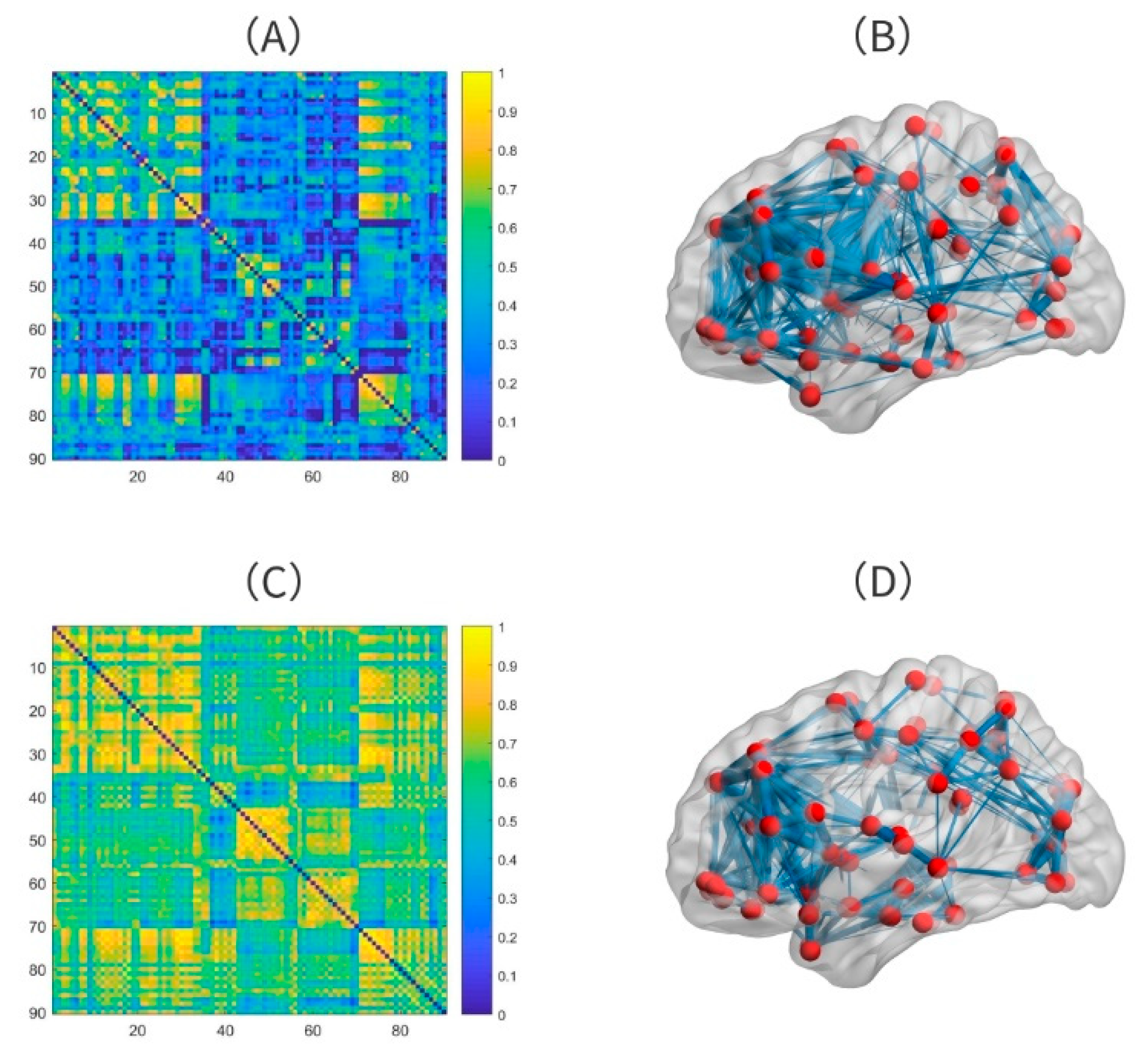
We extracted the correlation coefficient matrix from 106 subjects (59 patients with ASD and 46 NC controls). Figure 3 shows the functional and topological connectivity network of brain in a couple of ASD patient and normal controls. Next, we applied the feature selection algorithm we proposed to rank the importance of features. Then, the optimal feature subset was identified based on the SVM classifier, and the number of features that resulted in the best performance was 31. As shown in Table 2, the classification accuracy, sensitivity and specificity of the feature selection algorithm are 86.7%, 87.5% and 85.7%, respectively, which are obviously better than the results obtained by training the classifier with the original feature set.

3.2. The Optimal Feature Set and the Abnormal Brain Regions

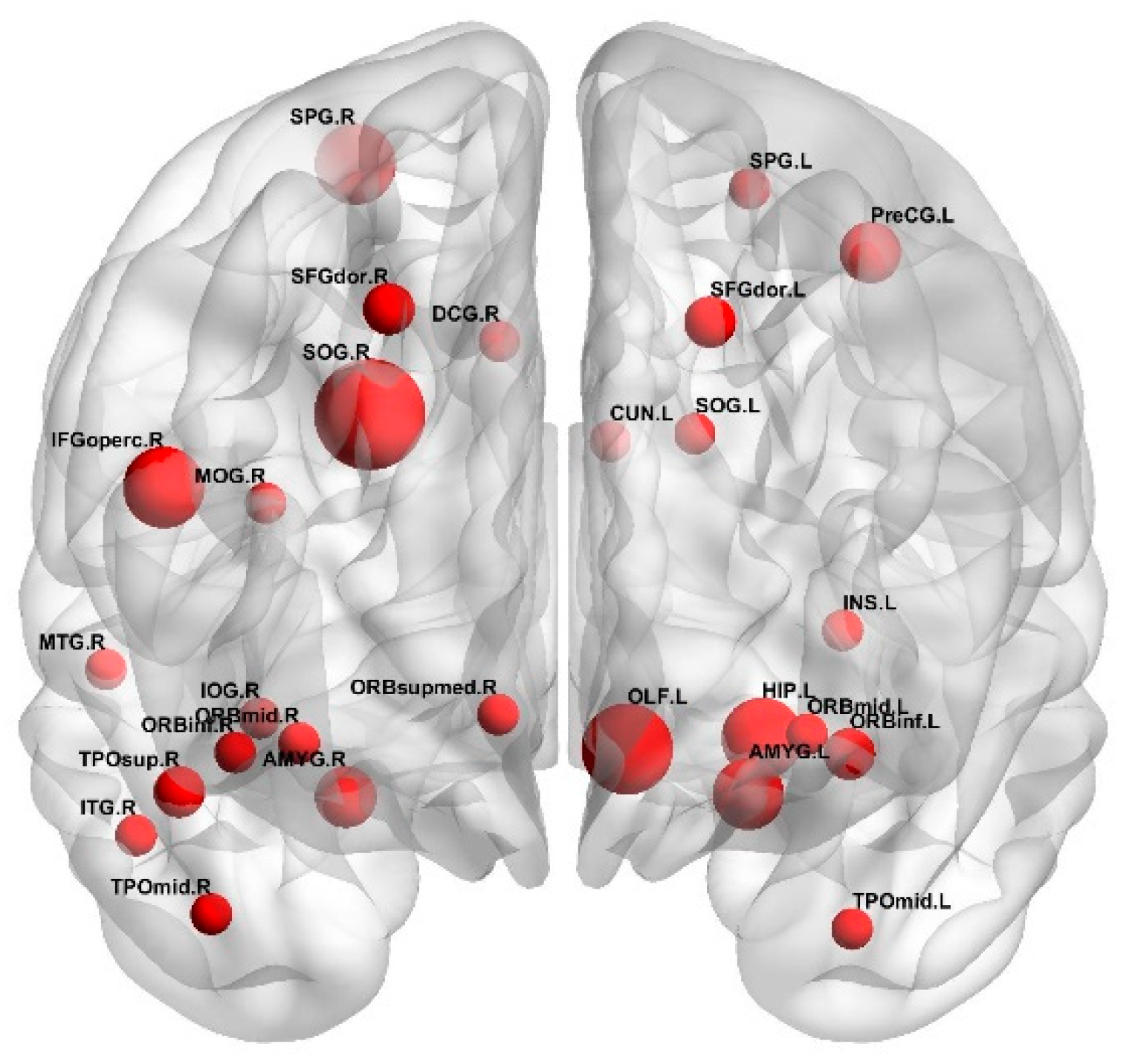
According to the feature selection algorithm we proposed, the number of features in the optimal feature subset is 31. We counted the number of occurrences of the brain regions connected by these 31 features and defined the number as the weight of the brain regions. Figure 4 shows the weight map of each brain region. Table 3 shows the brain regions with more frequent occurrences: the right superior occipital gyrus, the left olfactory cortex, the right inferior frontal gyrus (opercular part), the left hippocampus, the left amygdala, and the left precentral gyrus.

4. Discussion

4.1. Classification Effect

In this study, we used 5-fold cross-validation to assess the accuracy of the model corresponding to each feature subset. Based on the experimental results, the feature selection algorithm we proposed achieved a maximum accuracy of 86.7% when applied to the ASD diagnosis. In recent years, many researchers have proposed new feature selection algorithms and models for the diagnosis of ASD. For example, Chen [41] classified patients with ASD and TD individuals using support vector machine-recursive feature elimination (SVM-RFE) and achieved an accuracy of 66% in combination with a support vector machine. In a previous study [42], ASD was classified based on the differences in the interactions of different brain regions between patients with ASD and healthy controls. Through a nonlinear measurement of the interactions between time series pairs, the average classification accuracy ranged from 70% to 81%. A study [43] used a deep learning method based on an autoencoder to diagnose ASD with an accuracy of 70%. Research [44] proposed a recurrent neural network to integrate the phenotype data of the subjects with rs-fMRI data and extract features from them to diagnose patients with ASD, and their model reached an accuracy of 70.1%.
The classification accuracy of above models is usually not higher than 80%. Table 4 shows a comparison of the classification accuracy of our proposed method and the recently reported methods. When classifying patients with ASD, the selection of the optimal feature subset from the high-dimensional original feature set not only improves the classification accuracy but also contributes to improving our understanding of the brain abnormalities that cause the disease. Based on the analysis described above, the feature selection method based on the minimum spanning tree we proposed achieves a better diagnostic accuracy.

4.2. Comparison with Other Feature Selection Methods

We compared two other commonly used feature selection algorithms and the feature selection method we proposed on the same dataset to verify its effectiveness. One is the Fisher score feature selection method, which is a univariate feature selection method that is often used in supervised learning. Its main premise is to identify the feature subset in the feature set space that ensures the largest distance possible between data points of different categories and the smallest distance possible between data points of the same category. The other is the recursive feature elimination (RFE) method, which uses a base model for multiple rounds of training. After each round of training, the features of several weight coefficients are eliminated, and then the next round of training is conducted based on the new feature set. The methods used for comparison and our method all adopt the same experimental settings, including the same dataset, the same preprocessing method, the original feature set, the same classifier, and the same 5-fold cross-validation, to fairly compare the effects of the three feature selection methods. Table 5 shows the experimental results obtained using the three feature selection methods, and our proposed method displayed the highest classification accuracy. This analysis further confirms that the feature selection method we proposed exhibits good performance in diagnosing ASD.

4.3. Analysis of the Brain Regions with Greater Weight

Based on the experimental results, the superior occipital gyrus, olfactory cortex, inferior frontal gyrus (opercular part), and hippocampus are the main regions showing abnormalities in patients with ASD. Detailed descriptions of the analyses of these regions are presented below.
  • Superior occipital gyrus
Recent studies of structural and functional brain networks in patients with ASD suggest that cognitive deficits may be attributed to abnormal connections between different brain regions (such as the superior occipital gyrus) [45,46,47,48]. Consistent with the results of our study, the superior occipital gyrus of participants with autism showed significant abnormalities as the task complexity increased when participating in the test task compared with the normal control group [45]. In addition, based on the analysis of voxels between patients with ASD and normal controls, individuals with ASD present a significantly reduced grey matter volume in the superior occipital gyrus [49]. According to the experimental results, the region of the superior occipital gyrus appears more frequently, indicating that the superior occipital gyrus plays an important role in the recognition of ASD. This result is consistent with previous studies.
  • Olfactory cortex
Humans must rely on the olfactory cortex network in the brain to receive information from peripheral brain regions and then transmit the information back to the hippocampus to combine various discontinuous transient factors and form episodic and working memory. The olfactory cortex plays a crucial role in translating daily experiences into lasting memories. Many studies have pointed out that the olfactory cortex has a great influence on basic cognitive processes and is associated with a variety of mental disorders [50,51,52]. The symptoms of patients with autism include abnormal smell recognition, and 5% to 46% of patients with autism have been diagnosed with epilepsy; notably, the olfactory cortex is the key to smell recognition and a structure that leads to epilepsy [53]. In addition, based on a study of structural and functional magnetic resonance imaging of the olfactory changes in patients with ASD, alterations in olfaction in patients with ASD are rooted in the primary olfactory cortex [54]. Previous studies have further confirmed our results, and the olfactory cortex contributes to the identification of patients with ASD.
  • Inferior frontal gyrus
The frontal lobe is the most developed part of the brain, and it is responsible for thinking and calculation, and related to individual needs and emotions. The abnormal inferior frontal gyrus was found in several works of ASD research. For instance, Grezes et al. [55] and Philip et al. [56] discovered that activation of the inferior frontal gyrus in ASD patients decreased when doing the specific tasks. In another study, ASD patients appear to have lower activation in the right inferior frontal gyrus than normal controls when fearful faces were given to them [57]. In the process of facial expression recognition, patients with autism show hypoactivation of the inferior frontal gyrus. This activity gradually increases with age, while the activity of the control group does not [58]. In a recent study, patients with autism often failed to make accurate social judgments about others when their verbal and nonverbal expressions were inconsistent. Researchers explored the mechanism and finally found that the basic cause of impaired social judgment in patients with ASD was reduced brain activity in the inferior frontal gyrus [59]. The findings of these studies are consistent with our experimental results, indicating that the inferior frontal gyrus is an area of the brain showing abnormalities in patients with ASD.
  • Hippocampus
The hippocampus is located between the thalamus and the medial temporal lobe and is mainly responsible for the storage, conversion and orientation of long-term memory. In a study of memory impairment in patients with ASD, the connectivity between the hippocampus and other areas of the brain was significantly reduced in patients with ASD compared with normal controls, indicating that hippocampal damage is a key factor contributing to memory deficits in patients with ASD [60]. In addition, Mackiewicz et al. [61] discovered that the hippocampus was a key brain area involved in emotional memory. ASD patients were associated with changes in hippocampus volume [62]. In another study, the hippocampal volume of patients with ASD was larger than normal controls, indicating that ASD is related to the volume of the hippocampus [63]. Via et al. [64] found that the volume of gray matter in bilateral amygdala-hippocampus complex decreased significantly in ASD patients. In addition, the researchers extracted 11 features from the hippocampus of patients with ASD and the normal controls, and the two groups presented significantly different distributions of features and the features from the hippocampus had a strong ability to distinguish patients with ASD from the normal controls [65]. Thus, the hippocampus represents a potential biomarker for the diagnosis and characterization of ASD, consistent with the results of our experiments.

5. Conclusions

A feature selection method based on the minimum spanning tree was proposed in this study to automatically identify patients with ASD. First, we constructed an undirected graph from the original dataset and treated the features as nodes in the graph. The weight between nodes was determined by the redundancy between features and the discriminant ability of features. Second, we used the Prim algorithm to construct the minimum spanning tree. Finally, we combined the support vector machine algorithm to take the first N features with the highest classification accuracy as the optimal feature subset. Compared with other feature selection methods, our method exhibits better classification performance (accuracy rate of 86.7%). In the present study, we only used functional connections between different brain regions as features to identify patients with ASD. In future studies, we will use more features, such as graph theory features and dynamic connection features, in combination with the feature selection method proposed here to establish a better classification model. In addition, due to the limitation of the dataset, both ASD patients and NC may face the problem of imbalance in gender. In the next step, we will use more comprehensive data to solve the problem of data imbalance and detect the early patients.

Author Contributions

C.S. initiated the research and wrote the paper, J.Z. and X.W. supervised the research work and provided helpful suggestions. All authors have read and agreed to the published version of the manuscript.

Funding

This research was funded by the National Key Technologies RD Program (2017YFB1002502), and the General Program (61977010) of Nature Science Foundation of China.

Acknowledgments

The authors would like to thank all individuals who participated in the initial experiments from which raw data were collected.

Conflicts of Interest

The authors declare no conflict of interest.

References

  1. Frith, U.; Happé, F. Autism spectrum disorder. Curr. Biol. 2005, 15, R786–R790. [Google Scholar] [CrossRef] [Green Version]
  2. Kong, Y.; Gao, J.; Xu, Y.; Pan, Y.; Wang, J.; Liu, J. Classification of autism spectrum disorder by combining brain connectivity and deep neural network classifier. Neurocomputing 2019, 324, 63–68. [Google Scholar] [CrossRef]
  3. Zecavati, N.; Spence, S.J. Neurometabolic disorders and dysfunction in autism spectrum disorders. Curr. Neurol. Neurosci. Rep. 2009, 9, 129–136. [Google Scholar] [CrossRef]
  4. Amaral, D.G.; Schumann, C.M.; Nordahl, C.W. Neuroanatomy of autism. Trends Neurosci. 2008, 31, 137–145. [Google Scholar] [CrossRef]
  5. Khundrakpam, B.S.; Lewis, J.D.; Kostopoulos, P.; Carbonell, F.; Evans, A.C. Cortical Thickness Abnormalities in Autism Spectrum Disorders Through Late Childhood, Adolescence, and Adulthood: A Large-Scale MRI Study. Cereb. Cortex 2017, 27, 1721–1731. [Google Scholar] [CrossRef]
  6. Zablotsky, B.; Black, L.I.; Maenner, M.J.; Schieve, L.A.; Blumberg, S.J. Estimated prevalence of autism and other developmental disabilities following questionnaire changes in the 2014 national health interview survey. Natl. Health Stat. Rep. 2015, 87, 1–20. [Google Scholar]
  7. Karten, A.; Hirsch, J. Brief report: Anomalous neural deactivations and functional connectivity during receptive language in autism spectrum disorder: A functional MRI study. J. Autism Dev. Disord. 2015, 45, 1905–1914. [Google Scholar] [CrossRef]
  8. Fernell, E.; Eriksson, M.A.; Gillberg, C. Early diagnosis of autism and impact on prognosis: A narrative review. Clin. Epidemiol. 2013, 5, 33–43. [Google Scholar] [CrossRef] [PubMed] [Green Version]
  9. Mwangi, B.; Ebmeier, K.P.; Matthews, K.; Steele, J.D. Multi-centre diagnostic classification of individual structural neuroimaging scans from patients with major depressive disorder. Brain J. Neurol. 2012, 135, 1508–1521. [Google Scholar] [CrossRef] [PubMed] [Green Version]
  10. Plitt, M.; Barnes, K.A.; Martin, A. Functional connectivity classification of autism identifies highly predictive brain features but falls short of biomarker standards. NeuroImage Clin. 2015, 7, 359–366. [Google Scholar] [CrossRef] [PubMed] [Green Version]
  11. Bosl, W.J.; Tager-Flusberg, H.; Nelson, C.A. EEG Analytics for Early Detection of Autism Spectrum Disorder: A data-driven approach. Sci. Rep. 2018, 8, 6828. [Google Scholar] [CrossRef] [PubMed]
  12. Pereira, A.M.; Campos, B.M.; Coan, A.C.; Pegoraro, L.F.; de Rezende, T.J.R.; Obeso, I.; Dalgalarrondo, P.; da Costa, J.C.; Dreher, J.; Cendes, F. Differences in Cortical Structure and Functional MRI Connectivity in High Functioning Autism. Front. Neurol. 2018, 9, 539. [Google Scholar] [CrossRef] [Green Version]
  13. Van den Heuvel, M.P.; Hulshoff Pol, H.E. Exploring the brain network: A review on resting-state fMRI functional connectivity. Eur. Neuropsychopharmacol. 2010, 20, 519–534. [Google Scholar] [CrossRef]
  14. Bi, X.; Wang, Y.; Shu, Q.; Sun, Q.; Xu, Q. Classification of Autism Spectrum Disorder Using Random Support Vector Machine Cluster. Front. Genet. 2018, 9, 18. [Google Scholar] [CrossRef]
  15. Travers, B.G.; Adluru, N.; Ennis, C.; Tromp, D.P.M.; Destiche, D.; Doran, S.; Bigler, E.D.; Lange, N.; Lainhart, J.E.; Alexander, A.L. Diffusion tensor imaging in autism spectrum disorder: A review. Autism Res. 2012, 5, 289–313. [Google Scholar] [CrossRef] [Green Version]
  16. Ardekani, B.A.; Tabesh, A.; Sevy, S.; Robinson, D.G.; Bilder, R.M.; Szeszko, P.R. Diffusion tensor imaging reliably differentiates patients with schizophrenia from healthy volunteers. Hum. Brain Mapp. 2011, 32, 1–9. [Google Scholar] [CrossRef] [Green Version]
  17. Kaufmann, T.; Skåtun, K.C.; Alnæs, D.; Brandt, C.L.; Doan, N.T.; Agartz, I.; Melle, I.S.; Andreassen, O.A.; Westlye, L.T. Disintegration of sensorimotor brain networks in schizophrenia. Eur. Psychiatry 2016, 33, S33–S34. [Google Scholar] [CrossRef] [Green Version]
  18. Zhao, F.; Zhang, H.; Rekik, I.; An, Z.; Shen, D. Diagnosis of Autism Spectrum Disorders Using Multi-Level High-Order Functional Networks Derived From Resting-State Functional MRI. Front. Hum. Neurosci. 2018, 12, 184. [Google Scholar] [CrossRef]
  19. Jin, B.; Strasburger, A.; Laken, S.J.; Kozel, F.A.; Johnson, K.A.; George, M.S.; Lu, X. Feature selection for fMRI-based deception detection. BMC Bioinform. 2009, 10 (Suppl. 9), S15. [Google Scholar] [CrossRef] [Green Version]
  20. Guo, X.; Dominick, K.C.; Minai, A.A.; Li, H.; Erickson, C.A.; Lu, L.J. Diagnosing Autism Spectrum Disorder from Brain Resting-State Functional Connectivity Patterns Using a Deep Neural Network with a Novel Feature Selection Method. Front. Neurosci. 2017, 11, 460. [Google Scholar] [CrossRef]
  21. Dyrba, M.; Grothe, M.; Kirste, T.; Teipel, S.J. Multimodal analysis of functional and structural disconnection in Alzheimer’s disease using multiple kernel SVM. Hum. Brain Mapp. 2015, 36, 2118–2131. [Google Scholar] [CrossRef] [PubMed]
  22. Guo, H.; Cheng, C.; Cao, X.; Xiang, J.; Chen, J.; Zhang, K. Resting-state functional connectivity abnormalities in first-onset unmedicated depression. Neural Regen. Res. 2014, 9, 153–163. [Google Scholar] [PubMed]
  23. Fekete, T.; Wilf, M.; Rubin, D.; Edelman, S.; Malach, R.; Mujica-Parodi, L.R. Combining classification with fMRI-derived complex network measures for potential neurodiagnostics. PLoS ONE 2013, 8, e62867. [Google Scholar] [CrossRef] [PubMed] [Green Version]
  24. Bassett, D.S.; Nelson, B.G.; Mueller, B.A.; Camchong, J.; Lim, K.O. Altered resting state complexity in schizophrenia. Neuroimage 2012, 59, 2196–2207. [Google Scholar] [CrossRef] [PubMed] [Green Version]
  25. Arbabshirani, M.R.; Plis, S.; Sui, J.; Calhoun, V.D. Single subject prediction of brain disorders in neuroimaging: Promises and pitfalls. Neuroimage 2017, 145, 137–165. [Google Scholar] [CrossRef] [Green Version]
  26. Rakić, M.; Cabezas, M.; Kushibar, K.; Oliver, A.; Lladó, X. Improving the detection of autism spectrum disorder by combining structural and functional MRI information. NeuroImage Clin. 2020, 25, 102181. [Google Scholar] [CrossRef]
  27. Khazaee, A.; Ebrahimzadeh, A.; Babajani-Feremi, A. Identifying patients with Alzheimer’s disease using resting-state fMRI and graph theory. Clin. Neurophysiol. 2015, 126, 2132–2141. [Google Scholar] [CrossRef]
  28. Kang, J.; Han, X.; Song, J.; Niu, Z.; Li, X. The identification of children with autism spectrum disorder by SVM approach on EEG and eye-tracking data. Comput. Biol. Med. 2020, 120, 103722. [Google Scholar] [CrossRef]
  29. Fredo, A.J.; Jahedi, A.; Reiter, M.; Müller, R.A. Diagnostic classification of autism using resting-state fMRI data and conditional random forest. Age 2018, 12, 6–41. [Google Scholar]
  30. Eslami, T.; Mirjalili, V.; Fong, A.; Laird, A.R.; Saeed, F. ASD-DiagNet: A Hybrid Learning Approach for Detection of Autism Spectrum Disorder Using fMRI Data. Front. Neuroinform. 2019, 13, 70. [Google Scholar] [CrossRef]
  31. Li, G.; Liu, M.; Sun, Q.; Shen, D.; Wang, L. Early Diagnosis of Autism Disease by Multi-channel CNNs. Machine learning in medical imaging. MLMI (Workshop) 2018, 11046, 303–309. [Google Scholar]
  32. Di Martino, A.; Yan, C.; Li, Q.; Denio, E.; Castellanos, F.X.; Alaerts, K.; Anderson, J.S.; Assaf, M.; Bookheimer, S.Y.; Dapretto, M.; et al. The autism brain imaging data exchange: Towards a large-scale evaluation of the intrinsic brain architecture in autism. Mol. Psychiatry 2014, 19, 659–667. [Google Scholar] [CrossRef] [PubMed]
  33. Chao-Gan, Y.; Yu-Feng, Z. DPARSF: A MATLAB Toolbox for “Pipeline” Data Analysis of Resting-State fMRI. Front. Syst. Neurosci. 2010, 4, 13. [Google Scholar] [PubMed] [Green Version]
  34. Tzourio-Mazoyer, N.; Landeau, B.; Papathanassiou, D.; Crivello, F.; Etard, O.; Delcroix, N.; Mazoyer, B.; Joliot, M. Automated Anatomical Labeling of Activations in SPM Using a Macroscopic Anatomical Parcellation of the MNI MRI Single-Subject Brain. Neuroimage 2002, 15, 273–289. [Google Scholar] [CrossRef] [PubMed]
  35. Khazaee, A.; Ebrahimzadeh, A.; Babajani-Feremi, A. Application of advanced machine learning methods on resting-state fMRI network for identification of mild cognitive impairment and Alzheimer’s disease. Brain Imaging Behav. 2016, 10, 799–817. [Google Scholar] [CrossRef]
  36. You, Y.; Liang, D.; Wei, R.; Li, M.; Li, Y.; Wang, J.; Wang, X.; Jia, W.; Chen, T. Evaluation of metabolite-microbe correlation detection methods. Anal. Biochem. 2019, 567, 106–111. [Google Scholar] [CrossRef] [PubMed]
  37. Zhang, Y.; Dong, Z.; Phillips, P.; Wang, S.; Ji, G.; Yang, J.; Yuan, T. Detection of subjects and brain regions related to Alzheimer’s disease using 3D MRI scans based on eigenbrain and machine learning. Front. Comput. Neurosci. 2015, 9, 66. [Google Scholar] [CrossRef] [Green Version]
  38. Blennow, K.; Zetterberg, H. Cerebrospinal fluid biomarkers for Alzheimer’s disease. J. Alzheimer’s Dis. 2009, 18, 413–417. [Google Scholar] [CrossRef]
  39. Holtzman, D.M.; Morris, J.C.; Goate, A.M. Alzheimer’s disease: The challenge of the second century. Sci. Transl. Med. 2011, 3, 71s–77s. [Google Scholar] [CrossRef] [Green Version]
  40. Wang, C.; Xiao, Z.; Wu, J. Functional connectivity-based classification of autism and control using SVM-RFECV on rs-fMRI data. Physica Med. 2019, 65, 99–105. [Google Scholar] [CrossRef]
  41. Chen, C.P.; Keown, C.L.; Jahedi, A.; Nair, A.; Pflieger, M.E.; Bailey, B.A.; Müller, R. Diagnostic classification of intrinsic functional connectivity highlights somatosensory, default mode, and visual regions in autism. NeuroImage Clin. 2015, 8, 238–245. [Google Scholar] [CrossRef] [PubMed] [Green Version]
  42. DSouza, A.M.; Abidin, A.Z.; Wismüller, A. Classification of autism spectrum disorder from resting-state fMRI with mutual connectivity analysis. In Proceedings of the Medical Imaging 2019: Biomedical Applications in Molecular, Structural, and Functional Imaging, San Diego, CA, USA, 19–21 February 2019. [Google Scholar]
  43. Heinsfeld, A.S.; Franco, A.R.; Craddock, R.C.; Buchweitz, A.; Meneguzzi, F. Identification of autism spectrum disorder using deep learning and the ABIDE dataset. NeuroImage Clin. 2017, 17, 16–23. [Google Scholar] [CrossRef] [PubMed]
  44. Dvornek, N.C.; Ventola, P.; Duncan, J.S. Combining phenotypic and resting-state fmri data for autism classification with recurrent neural networks. In Proceedings of the IEEE International Symposium on Biomedical Imaging, Washington, DC, USA, 4–7 April 2018. [Google Scholar]
  45. Simard, I.; Luck, D.; Mottron, L.; Zeffiro, T.A.; Soulières, I. Autistic fluid intelligence: Increased reliance on visual functional connectivity with diminished modulation of coupling by task difficulty. NeuroImage Clin. 2015, 9, 467–478. [Google Scholar] [CrossRef] [PubMed] [Green Version]
  46. Ha, S.; Sohn, I.; Kim, N.; Sim, H.J.; Cheon, K. Characteristics of Brains in Autism Spectrum Disorder: Structure, Function and Connectivity across the Lifespan. Exp. Neurobiol. 2015, 24, 273–284. [Google Scholar] [CrossRef] [PubMed] [Green Version]
  47. Keown, C.L.; Shih, P.; Nair, A.; Peterson, N.; Mulvey, M.E.; Müller, R. Local functional overconnectivity in posterior brain regions is associated with symptom severity in autism spectrum disorders. Cell Rep. 2013, 5, 567–572. [Google Scholar] [CrossRef] [PubMed] [Green Version]
  48. Xu, S.; Li, M.; Yang, C.; Fang, X.; Ye, M.; Wei, L.; Liu, J.; Li, B.; Gan, Y.; Yang, B.; et al. Altered Functional Connectivity in Children With Low-Function Autism Spectrum Disorders. Front. Neurosci. 2019, 13, 806. [Google Scholar] [CrossRef] [Green Version]
  49. Ecker, C.; Suckling, J.; Deoni, S.C.; Lombardo, M.V.; Bullmore, E.T.; Baron-Cohen, S.; Catani, M.; Jezzard, P.; Barnes, A.; Bailey, A.J.; et al. Brain anatomy and its relationship to behavior in adults with autism spectrum disorder: A multicenter magnetic resonance imaging study. Arch. Gen. Psychiatry 2012, 69, 195–209. [Google Scholar] [CrossRef] [Green Version]
  50. Turetsky, B.I.; Hahn, C.; Borgmann-Winter, K.; Moberg, P.J. Scents and nonsense: Olfactory dysfunction in schizophrenia. Schizophr. Bull. 2009, 35, 1117–1131. [Google Scholar] [CrossRef] [Green Version]
  51. Moberg, P.J.; Agrin, R.; Gur, R.E.; Gur, R.C.; Turetsky, B.I.; Doty, R.L. Olfactory dysfunction in schizophrenia: A qualitative and quantitative review. Neuropsychopharmacology 1999, 21, 325–340. [Google Scholar] [CrossRef] [Green Version]
  52. Soudry, Y.; Lemogne, C.; Malinvaud, D.; Consoli, S.; Bonfils, P. Olfactory system and emotion: Common substrates. Eur. Ann. Otorhinolaryngol. Head Neck Dis. 2011, 128, 18–23. [Google Scholar] [CrossRef] [Green Version]
  53. Menassa, D.A.; Sloan, C.; Chance, S.A. Primary olfactory cortex in autism and epilepsy: Increased glial cells in autism. Brain Pathol. 2017, 27, 437–448. [Google Scholar] [CrossRef] [PubMed]
  54. Koehler, L.; Fournel, A.; Albertowski, K.; Roessner, V.; Gerber, J.; Hummel, C.; Hummel, T.; Bensafi, M. Impaired Odor Perception in Autism Spectrum Disorder Is Associated with Decreased Activity in Olfactory Cortex. Chem. Senses 2018, 43, 627–634. [Google Scholar] [CrossRef] [PubMed]
  55. Grèzes, J.; Wicker, B.; Berthoz, S.; de Gelder, B. A failure to grasp the affective meaning of actions in autism spectrum disorder subjects. Neuropsychologia 2009, 47, 1816–1825. [Google Scholar] [CrossRef] [PubMed]
  56. Philip, R.C.M.; Whalley, H.C.; Stanfield, A.C.; Sprengelmeyer, R.; Santos, I.M.; Young, A.W.; Atkinson, A.P.; Calder, A.J.; Johnstone, E.C.; Lawrie, S.M.; et al. Deficits in facial, body movement and vocal emotional processing in autism spectrum disorders. Psychol. Med. 2010, 40, 1919–1929. [Google Scholar] [CrossRef] [PubMed] [Green Version]
  57. Kim, S.; Choi, U.; Park, S.; Oh, S.; Yoon, H.; Koh, Y.; Im, W.; Park, J.; Song, D.; Cheon, K.; et al. Abnormal activation of the social brain network in children with autism spectrum disorder: An FMRI study. Psychiatry Investig. 2015, 12, 37–45. [Google Scholar] [CrossRef] [Green Version]
  58. Bastiaansen, J.A.; Thioux, M.; Nanetti, L.; van der Gaag, C.; Ketelaars, C.; Minderaa, R.; Keysers, C. Age-related increase in inferior frontal gyrus activity and social functioning in autism spectrum disorder. Biol. Psychiatry 2011, 69, 832–838. [Google Scholar] [CrossRef]
  59. Watanabe, T.; Yahata, N.; Abe, O.; Kuwabara, H.; Inoue, H.; Takano, Y.; Iwashiro, N.; Natsubori, T.; Aoki, Y.; Takao, H.; et al. Diminished medial prefrontal activity behind autistic social judgments of incongruent information. PLoS ONE 2012, 7, e39561. [Google Scholar] [CrossRef] [Green Version]
  60. Cooper, R.A.; Richter, F.R.; Bays, P.M.; Plaisted-Grant, K.C.; Baron-Cohen, S.; Simons, J.S. Reduced Hippocampal Functional Connectivity during Episodic Memory Retrieval in Autism. Cereb. Cortex 2017, 27, 888–902. [Google Scholar] [CrossRef] [Green Version]
  61. Mackiewicz, K.L.; Sarinopoulos, I.; Cleven, K.L.; Nitschke, J.B. The effect of anticipation and the specificity of sex differences for amygdala and hippocampus function in emotional memory. Proc. Natl. Acad. Sci. USA 2006, 103, 14200–14205. [Google Scholar] [CrossRef] [Green Version]
  62. Mailo, J.; Tang-Wai, R. Insight into the precuneus: A novel seizure semiology in a child with epilepsy arising from the right posterior precuneus. Epileptic Disord. 2015, 17, 321–327. [Google Scholar] [CrossRef]
  63. Reinhardt, V.P.; Iosif, A.; Libero, L.; Heath, B.; Rogers, S.J.; Ferrer, E.; Nordahl, C.; Ghetti, S.; Amaral, D.; Solomon, M. Understanding Hippocampal Development in Young Children With Autism Spectrum Disorder. J. Am. Acad. Child Adolesc. Psychiatry 2020, 59, 1069–1079. [Google Scholar] [CrossRef] [PubMed]
  64. Via, E.; Radua, J.; Cardoner, N.; Happé, F.; Mataix-Cols, D. Meta-analysis of gray matter abnormalities in autism spectrum disorder: Should Asperger disorder be subsumed under a broader umbrella of autistic spectrum disorder? Arch. Gen. Psychiatry 2011, 68, 409–418. [Google Scholar] [CrossRef] [PubMed] [Green Version]
  65. Chaddad, A.; Desrosiers, C.; Hassan, L.; Tanougast, C. Hippocampus and amygdala radiomic biomarkers for the study of autism spectrum disorder. BMC Neurosci. 2017, 18, 52. [Google Scholar] [CrossRef] [PubMed] [Green Version]
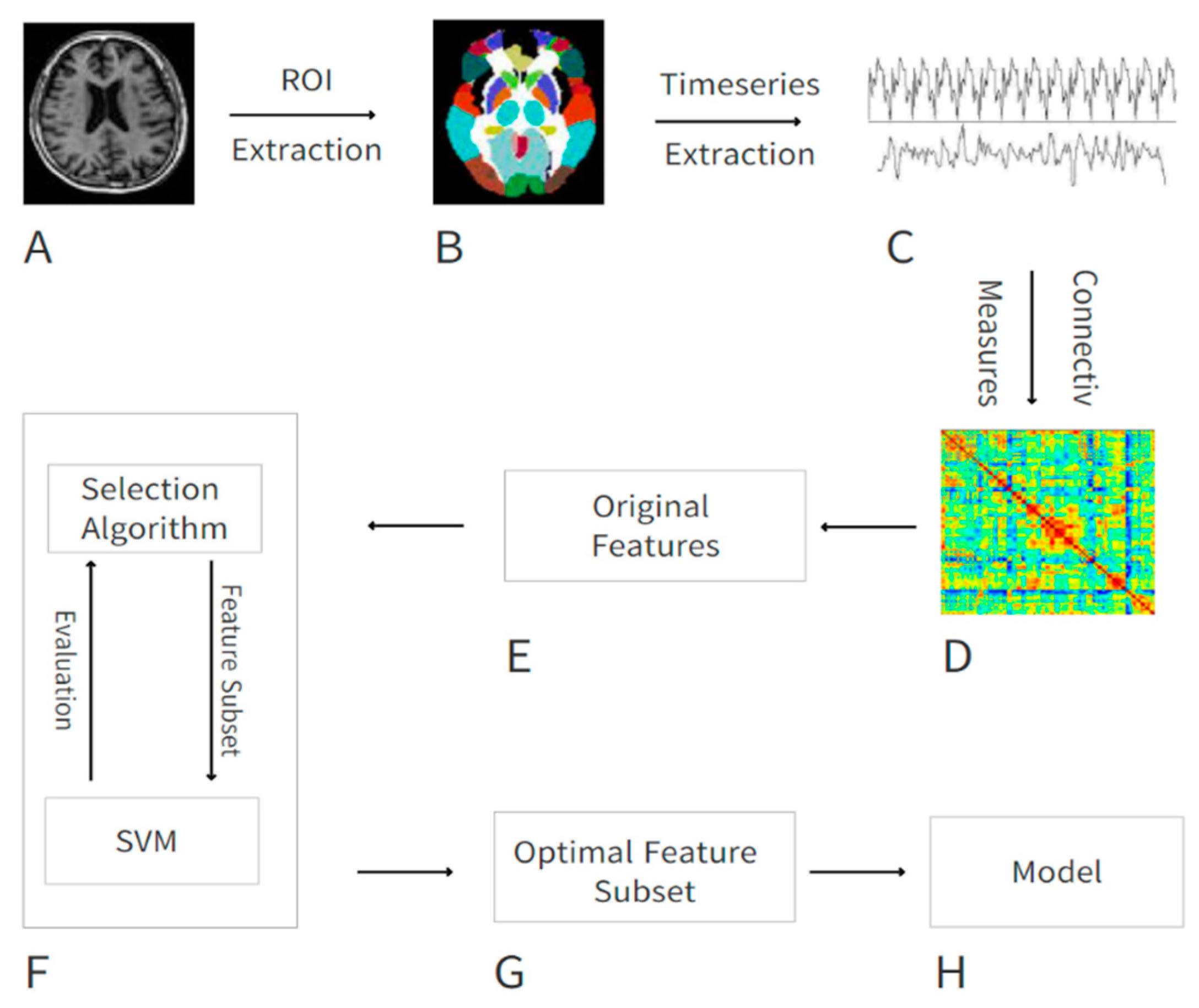
Figure 1. Graphical framework of the computational pipeline. (A) Raw functional magnetic resonance images (fMRI) images of subjects; (B) after preprocessing the brain is divided into 90 regions of interest (ROI); (C) by averaging the BOLD activity in each ROI, a time series is extracted representing brain activity in that region; (D) using different measures of connectivity, a connectivity matrix is generated from the ROI time series quantifying the connectivity level between individual ROIs; (E) the upper triangular elements in the connectivity matrix are flattened into a feature vector, which constitutes the original features; (F) our proposed feature selection method is applied to choose a handful of features that contribute to the highest classification accuracy; (G,H) the resulting optimal feature subset is passed to a SVM which trains a model to identify autism spectrum disorder (ASD).
Symmetry 12 01995 g001
Figure 2. The weight graph of N dimensional feature vectors.
Symmetry 12 01995 g002
Figure 3. Functional and topology connectivity network. The connectivity matrix (A) and topology (B) of a representative normal control are shown. (C,D) are the connectivity matrix and topological connectivity network of a representative ASD patient, respectively.
Symmetry 12 01995 g003
Figure 4. The weight of each brain region. Circles represent Automatic Anatomical Labeling (AAL) regions and the larger the circle, the greater the weight.
Symmetry 12 01995 g004
Table 1. Basic information of ASD and normal controls (NC).
Variables   ( Mean   ±   SD ) Autism (n = 59)NC (n = 46)p Value
Gender(M/F)51/839/70.81
Age(years)12.47   ±   2.312.35   ±   1.90.77
Table 2. Comparison of classification results between the optimal feature subset and the original feature set.
Feature SetAccuracy (%)Sensitivity (%)Specificity (%)
Optimal feature subset86.787.585.7
Original feature set57.161.550
Table 3. The brain regions with higher weight. Abbreviations: SOG.R, Superior occipital gyrus; OLF.L, Olfactory cortex; IFGoperc.R, Inferior frontal gyrus, opercular part; HIP.L, Hippocampus; AMYG.L, Amygdala; PreCG.L, Precental gyrus.
WeightRegion
8SOG.R
6OLF.L
5IFGoperc.R HIP.L
4AMYG.L
3PreCG.L
Table 4. Accuracy comparison of proposed method and state-of-the-art classification methods.
MethodsAccuracy (%)
Chen et al. [39]66
Adora et al. [40]70–81
Anibal et al. [41]70
Nicha et al. [42]70.1
Our method86.7
Table 5. Comparison of classification results between the three feature selection methods.
Feature SetAccuracy (%)Sensitivity (%)Specificity (%)
Fisher score64.387.566.7
RFE68.883.360
Our method86.787.585.7
Publisher’s Note: MDPI stays neutral with regard to jurisdictional claims in published maps and institutional affiliations.