Article

Efficacious Analytical Technique Applied to Fractional Fornberg–Whitham Model and Two-Dimensional Fractional Population Model

Department of Mathematics, University of Hafr Al Batin, Hafar Al Batin 39524, Saudi Arabia
Symmetry 2020, 12(12), 1976; https://doi.org/10.3390/sym12121976
Submission received: 18 September 2020 / Revised: 9 November 2020 / Accepted: 10 November 2020 / Published: 30 November 2020

Abstract

:
This paper presents an efficacious analytical and numerical method for solution of fractional differential equations. This technique, here in named q-HATM (q-homotopy analysis transform method) is applied to a one-dimensional fractional Fornberg–Whitham model and a two-dimensional fractional population model emanating from biological sciences. The overwhelming agreement of our analytical solution by the q-HATM technique with the exact solution indeed establishes the efficacy of q-HATM to solve the fractional Fornberg–Whitham model and the two-dimensional fractional population model. Furthermore, comparisons by means of extensive analysis using numerics, graphs and error analysis are presented to affirm the preference of q-HATM technique over other methods. A variant of the q-HATM using symmetry can also be considered to solve these problems.

1. Introduction

The 17th century ushered in the discovery of calculus independently by both Gottfried Wilhelm Leibniz and Isaac Newton, with the former introducing the symbol D n f = d n f d x n , meaning the nth derivative of a function f, where n is a nonnegative integer. L’Hôpital, out of curiosity, had asked Leibniz if n could be allowed to take a fractional value. This question by l’Hôpital to Leibniz was going to become a future field of mathematics to find applications in different areas of human endeavors. For more on the history of fractional calculus, see [1] and references therein. Fractional calculus indeed comprises both fractional integrals and fractional derivatives. Its numerous applications have enticed many scientists and engineers to pay more attention to it in recent years. Practical applications were found in image and signal processing [2,3], biotechnology [4], nanotechnology [5] and viscoelasticity [6]. For more applications of fractional calculus, see [7,8,9,10,11,12,13,14,15,16,17,18,19,20], and more recently, [21,22,23,24,25,26,27,28,29,30,31,32,33,34,35,36,37,38,39,40]. It is extremely difficult in general to obtain an exact solution (in terms of a handy function) for a fractional differential equation. Therefore, several analytical methods were derived in order to find approximate solutions. This, in itself, raises the challenge of always trying to get an analytical solving method which is efficient, reliable, produces better approximations and guarantees faster rate of convergence. Thus, several methods have been proposed; these are the variational iteration method (VIM), Adomian’s decomposition method (ADM), the homotopy analysis method (HAM), the homotopy perturbation method (HPM), the differential transform method (DTM), the new iteration method (NIM), the least-squares residual power series method (LSRPSM), the residual power series method (RPSM) and several others. In 1992, Liao [41,42] introduced the HAM to solve fractional differential equations. However, there was still a need for another method that could guarantee faster convergence and give a more accurate approximation. This led to the proposition of a modification of the HAM to q-HAM, which uses the axillary parameter q to obtain a more refined approximate solution [10]. Solutions to some nonlinear fractional differential equations were obtained using q-HAM; see [12,13,14,28,32,43,44]. Recently, Singh et al. [30] introduced the q-homotopy analysis transform method (q-HATM). Actually, the q-HATM was derived from the combination of the Laplace transform and the q-HAM. This combination is an improvement on the q-HAM, in that some properties of the equation under consideration are still maintained as the q-HATM sorts for an approximate solution in a series form. The q-HATM also has an added advantage as it deploys a convergence parameter , which is effectively selected to guarantee faster convergence to the solution, gives a better degree of accuracy and provides adjustment and control of convergence regions. A number of researchers have solved various nonlinear fractional differential equations by using the q-HATM [31,33,34,45,46,47]. In contrast to some other methods, q-HATM does not need any sort of discretization or perturbation. It also does not need polynomials like in ADM and the homotopy perturbation transform method (HPTM), nor is a Lagrange multiplier needed as in the case of the VIM. In light of the aforementioned advantages that q-HATM brings to the fore, in this work, we sort to find approximate solutions by applying the q-HATM first to the Fornberg–Whitham equation and secondly to a fractional biological population model in two dimensions.
In mathematical physics, the Fornberg–Whitham equation is a significant model used in investigating the qualitative behavior of wave breaking [36]. It is given as
φ t φ x x t + φ x = φ φ x x x φ φ x + 3 φ x φ x x ,
where φ ( x , t ) is the velocity of fluid. A peaked solution to Equation (1) was derived by Fornberg and Whitham [11] and is given as φ ( x , t ) = K e x 2 2 t 3 , where K is an arbitrary constant. Considering the enormous application of fractional calculus to diverse fields of sciences, researchers recently introduced the fractional derivative to obtain the following time-fractional Fornberg–Whitham equation
D t α φ φ x x t + φ x = φ φ x x x φ φ x + 3 φ x φ x x , 0 < α 1 , t > 0 ,
where D t α represents the Caputo derivative in the variable t of order α . Various analytical approaches and methods have been employed by different authors in other to solve the classical Fornberg–Whitham equation (Equation (1)) (see [48,49]) and fractional Fornberg–Whitham equation (Equation (2)) (see [26,29,50,51,52,53]). Considering the simplicity in implementation, efficiency and reliability of the q-HATM (see [54]), we apply the q-HATM to solve Equation (2); then, taking advantage of the presence of a convergence parameter , we obtain a faster and more accurate approximate solution in few iterations. Our applied method outperformed existing methods that have been applied to solve Equation (2), in terms of ease of computations, faster convergence rate and more accurate approximate solution.
Secondly, we demonstrate the preference of the q-HATM over other methods in solving the time-fractional biological population model,
D t α φ ( x , y , t ) φ x x 2 ( x , y , t ) φ y y 2 ( x , y , t ) λ φ ( x , y , t ) = 0 , 0 < α 1 , t > 0 ,
where D t α represents the Caputo derivative in the variable t of order α .
We organized the paper as follows. In Section 2, we present some basic tools needed in this work. Analysis of the q-HATM is given in Section 3. Application of the q-HATM to the fractional Fornberg–Whitham equation is presented in Section 4. Application of the q-HATM to a fractional biological population model is presented in Section 5. Final remarks are stated in Section 6.

2. Preliminaries

In this section, we present some basic tools that will be used hereafter.
Definition 1 
(Riemann–Liouville integral). Given a function φ C m , m 1 , the Riemann–Liouville fractional integral of order α 0 of φ is defined as [55,56,57]
J α φ ( t ) = 1 Γ ( α ) 0 t ( t η ) α 1 φ ( η ) d η , α , t > 0
where J 0 φ ( t ) = φ ( t ) and Γ is the known regular gamma function.
Definition 2 
(Caputo derivative). The fractional derivative of the function φ of order α, for n 1 < α n , n N in the sense of Caputo is defined as [56,57]
D t α φ ( t ) : = φ ( n ) ( t ) , α = n , J n α φ ( n ) ( t ) , n 1 < α < n ,
where
J n α φ ( n ) ( t ) = 1 Γ ( n α ) 0 t ( t η ) n α 1 φ ( n ) ( η ) d η , α , t > 0 .
The Caputo derivative (Equation (5)) has the following properties:
(a)
D t α ( δ 1 φ ( t ) + δ 2 φ ( t ) ) = δ 1 D t α φ ( t ) + δ 2 D t α φ ( t ) , δ 1 , δ 2 R ,
(b)
D t α J α φ ( t ) = φ ( t ) ,
(c)
J α D t α φ ( t ) = φ ( t ) k = 0 n 1 φ ( k ) ( t ) t k k ! .
Definition 3 
(Laplace transform). The Laplace transform of the Caputo fractional derivative D t α φ ( t ) is given as [55,58]
L t D t α φ ( t ) = s α L t [ φ ( t ) ] k = 0 n 1 s α k 1 φ ( k ) ( 0 + ) , n 1 < α n .

3. The q -HATM Technique

The general procedure and techniques for applying the q-HATM to an abstract nonlinear differential equation are presented here. Given the following abstract nonlinear time-fractional differential equation
D t α φ ( x , t ) + G ( φ ( x , t ) ) + N ( φ ( x , t ) ) = g ( x , t ) , n 1 < α n ,
where D t α is the Caputo fractional derivative, G is a linear differential operator, N is a nonlinear differential operator, g is the source term and φ is the unknown function, we apply the Laplace transform in the variable t to both sides of Equation (7); keeping in mind Equation (6), we get
L t [ φ ( x , t ) ] 1 s α j = 0 n 1 s α j 1 φ ( j ) ( x , 0 ) + 1 s α L t [ G ( φ ( x , t ) ) + N ( φ ( x , t ) ) g ( x , t ) ] = 0 .
For 0 q 1 , according to the homotopy method [41], the so-called zeroth-order deformation is given as
( 1 q ) L t ( ψ ( x , t ; q ) φ 0 ( x , t ) ) = q H ( x , t ) Υ [ ψ ( x , t ; q ) ] ,
where
Υ [ ψ ( x , t ; q ) ] : = L t [ ψ ( x , t ; q ) ] 1 s α j = 0 n 1 s α j 1 ψ ( j ) ( x , 0 ; q ) + 1 s α L t [ G ( ψ ( x , t ; q ) ) + N ( ψ ( x , t ; q ) ) g ( x , t ) ] .
H ( x , t ) 0 represents an auxiliary function, is an auxiliary parameter and q is an embedded parameter. It is easy to see that when q = 0 and q = 1 , then from Equation (9), we can obtain, respectively,
ψ ( x , t ; 0 ) = φ 0 ( x , t ) a n d ψ x , t , q = φ ( x , t ) .
It follows according to Equation (11) that the solution ψ ( x , t ; q ) of Equation (9) ranges from the initial guess φ 0 ( x , t ) to the solution φ ( x , t ) of Equation (7) as q ranges from 0 to 1. Then, one chooses an appropriate H such that the solution ψ ( x , t ; q ) of Equation (9) is valid on 0 q 1 . Next, with Equation (11) in mind, and the appropriate choice of H , we can expand ψ ( x , t ; q ) in Taylor series [59] about q = 0 to get
ψ ( x , t ; q ) = φ 0 ( x , t ) + k = 1 φ k ( x , t ) q k ,
such that Equation (12) converges at q = 1 , where
φ k ( x , t ) = 1 k ! k ψ ( x , t , q ) q k | q = 0 ;
see [41] and references therein. It follows that
φ ( x , t ) = φ 0 ( x , t ) + k = 1 φ k ( x , t ) q k .
Performing k-times differentiation of Equation (9) with respect to q, then evaluating at q = 0 and dividing through by k ! , we get
L t φ k ( x , t ) η k * φ k 1 ( x , t ) = H ( x , t ) k ( φ k 1 ( x , t ) ) ,
where the vector φ ( x , t ) is given as
φ ( x , t ) = { φ j ( x , t ) } j = 0 k ,
with
k ( φ k 1 ( x , t ) ) = L t [ φ k 1 ( x , t ) ] 1 η k * j = 0 n 1 s α j 1 φ ( j ) ( x , 0 ) + 1 s α L t [ g ( x , t ) ] + 1 s α L t G ( φ ( x , t ) ) + H k 1
and
η k * : = 0 , k 1 , 1 , o t h e r w i s e .
In Equation (16), H k is given as
H k = 1 k ! k ψ ( x , t , q ) q k | q = 0 ,
where
ψ ( x , t , q ) = ψ 0 + q ψ 1 + q 2 ψ 2 + q 3 ψ 3 +
is the homotopy polynomial.
Application of the inverse Laplace transform to Equation (15) yields
φ k ( x , t ) = η k * φ k 1 ( x , t ) + L t 1 H ( x , t ) k ( φ k 1 ( x , t ) ) .
For the convergence analysis of the q-HATM, we present the following theorems; their proofs are given in [10,34,46].
Theorem 1 
(Convergence of q-HATM [34,46]). Let T : B B be a nonlinear contraction mapping on a Banach space B , i.e., there exists 0 < K < 1 such that
T ( φ ) T ( φ ˜ ) K φ φ ˜ , φ , φ ˜ B .
By the Banach’s fixed point theorem [60], for any φ 0 , φ ˜ 0 B , the sequence { φ k } generated by the q-HATM converges to a fixed point of T . Furthermore,
φ i φ k K k 1 K φ 1 φ 0 .
Theorem 2 
(Error analysis [10,34]). Assume that the series solution
k = 0 φ k ( x , t ) q k
given by Equation (14) converges to φ ( x , t ) the solution of Equation (7) for specified values of ℏ. Suppose there exists a real number 0 < ε < 1 such that
φ j + 1 ( x , t ) ε φ j ( x , t ) , j .
If the sequence of partial sums
φ ( N ) ( x , t ; q ; ) = k = 0 N φ k ( x , t ) q k
is used as an approximation to the solution φ ( x , t ) of Equation (7), then the absolute error is bounded as follows
φ ( x , t ) φ ( N ) ( x , t ; q ; ) ε N + 1 1 ε φ 0 ( x , t ) .
Remark 1. 
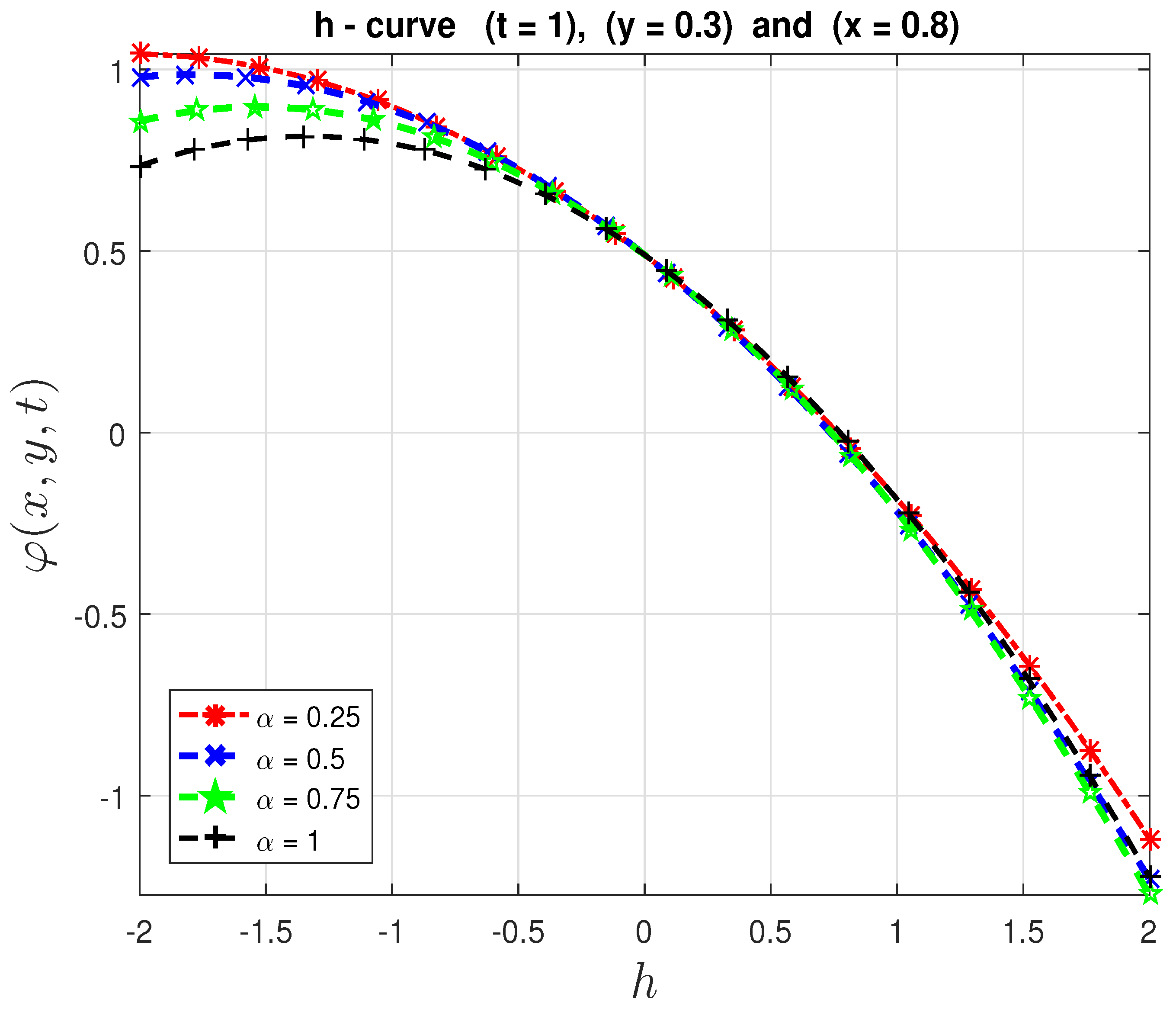
A critical part of the q-HATM technique lies in the appropriate and careful choice of ℏ which guarantees faster convergence of the approximate solution to the exact solution and greatly minimizes the absolute error. A classical way to find the best ℏ is by the use of the well-known ℏ-curves. The ℏ-curve is drawn using certain quantities of the solution versus ℏ. The best choice of the convergence control parameter ℏ is carefully made using the horizontal line test. This approach works quite well when an exact solution for a particular α value is known. However, in the case where no exact solution is known, there are different other ways to obtain a best ℏ that guarantees faster and better convergence. One method is to minimize, with respect to ℏ, the norm of the discrete residual function at each order of HAM approximation [61]. Another approach is by applying optimization method to minimize the residual of the mth-order approximate solutions, with respect to the homotopy parameter ℏ [37]. Hence, systematically, the optimal choice of ℏ that minimizes error and gives better convergence speed at every order of HAM approximation can be obtained. See also [62] (Chapter 4) and [35] for other methods to obtain ℏ.

4. Application to the Fractional Fornberg–Whitham Equation

In this section, we apply the q-HATM to solve the Caputo time-fractional Fornberg–Whitham equation and compare our results with those obtained from other methods. Recently, in [63], LSRPSM was used to obtain an approximate solution for the fractional Fornberg–Whitham equation. It was established that LSRPSM outperformed other methods such as RPSM and VIM in terms of accuracy and rate of convergence. We consider the following fractional Fornberg–Whitham equation:
D t α φ φ x x t + φ x = φ φ x x x φ φ x + 3 φ x φ x x , 0 < α 1 , t > 0 ,
with the initial data
φ ( x , 0 ) = 4 3 e x p x 2 .
The exact solution to Equation (19) when α = 1 is given as
φ ( x , t ) = 4 3 e x p x 2 2 t 3 .
We take the Laplace transform (in variable t) of Equation (19) and, keeping in mind Equation (20), we get
L t φ 1 s φ ( x , 0 ) + 1 s α 2 φ x 2 ( x , 0 ) 1 s α 1 L t 2 φ x 2 + 1 s α L t φ x φ 3 φ x 3 + φ φ x 3 φ x 2 φ x 2 = 0 .
Taking ψ ( x , t ; q ) , we define the nonlinear function
Υ ( ψ ( x , t ; q ) ) = L t ψ 1 s ψ ( x , t ; 0 ) + 1 s α 2 ψ x 2 ( x , t ; 0 ) 1 s α 1 L t 2 ψ x 2 + 1 s α L t ψ x ψ 3 ψ x 3 + ψ ψ x 3 ψ x 2 ψ x 2 .
From Equation (15), taking H 1 , the kth-order deformation equation is given as
L t φ k η k * φ k 1 = k ( φ k 1 ) ,
where
k ( φ k 1 ) = L t φ k 1 1 η k * 4 3 s e x / 2 1 3 s α e x / 2 1 s α 1 L t 2 φ k 1 x 2 + 1 s α 1 L t φ k 1 x j = 0 k 1 φ j 3 φ k 1 j x 3 + j = 0 k 1 φ j φ k 1 j x 3 j = 0 k 1 φ j x 2 φ k 1 j x 2 .
Taking the inverse Laplace transform of Equation (23), we get
φ k = η k * φ k 1 + L t 1 k ( φ k 1 ) .
Therefore, making use of Equations (17) and (24) in Equation (25), we obtain the following iterations for the approximate solution:
φ 0 ( x , t ) = 4 3 e x / 2 , φ 1 ( x , t ) = 2 t α e x / 2 3 Γ ( α + 1 ) , φ 2 ( x , t ) = ( 1 + h ) φ 1 + t α 1 e x / 2 3 Γ ( α ) 2 t 2 α 1 e x / 2 6 Γ ( 2 α ) + 2 t 2 α e x / 2 3 Γ ( 2 α + 1 ) .
Using Equation (26), we consider as our approximate solution the sequence of partial sums
φ ( 2 ) ( x , t ) = k = 0 2 φ k ( x , t ) q k .
Thus, taking q = 1 , the approximate solution φ ( 2 ) ( x , t ) of Equation (19) is
φ ( 2 ) ( x , t ) = 4 e x / 2 3 + t α 1 e x / 2 3 Γ ( α ) 2 t 2 α 1 e x / 2 6 Γ ( 2 α ) + 2 t α e x / 2 3 Γ ( α + 1 ) + 2 ( 1 + ) t α e x / 2 3 Γ ( α + 1 ) + 2 t 2 α e x / 2 3 Γ ( 2 α + 1 ) .

Numerical Comparison

In Table 1, we present numerical results (when α = 1 ) for some values of t and x. The solutions obtained using the exact solution (Equation (25)), the q-HATM solution (Equation (27)) and absolute errors for the q-HATM and other methods (the LSRPSM [63], the RPSM [63] and the VIM [26]) are tabulated. In Table 1, “itr” means the number of iterations performed for the particular method. Table 2 shows different numerical results obtained by the q-HATM for different values of α ( α = 0.25 , 0.5 , 0.75 ), with x = 5 , 5 and t = 0.1 , 0.2 , 0.3 , 0.4 , 0.5 .
Remark 2. 
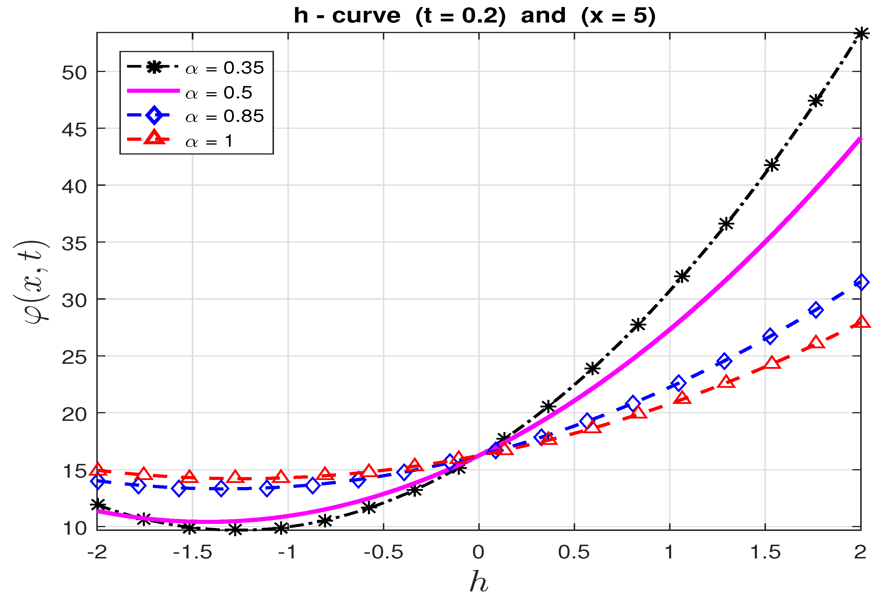
Observe that from Equation (26), we have only performed two iterations of the q-HATM. Moreover, as could be seen from Table 1, when α = 1 , and taking = 1.28 (according to Figure 1), the numerical solution obtained by the q-HATM has a far-reaching match to the exact solution (with smallest absolute error) when compared to other methods presented in the table. Only in the case when t = 0.5 is the absolute error for the LSRPSM lesser than that of the q-HATM for this problem. Hence, with few iterations, our solution obtained by the q-HATM best approximates the exact solution to a high and appreciable number of significant digits. Moreover, the computations required to obtain our approximate solution φ ( 2 ) ( x , t ) are less strenuous compared to those of the LSRPSM [63], the RPSM [63] and the VIM [26].
Remark 3. 
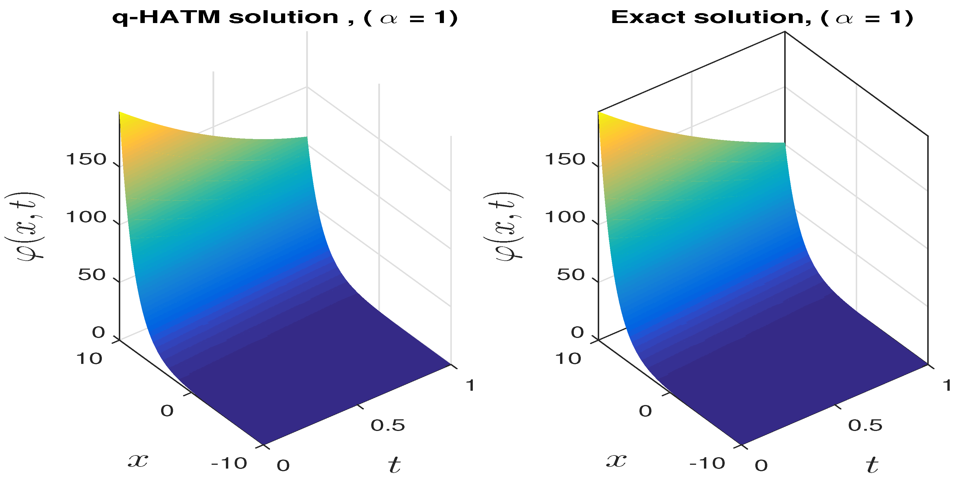
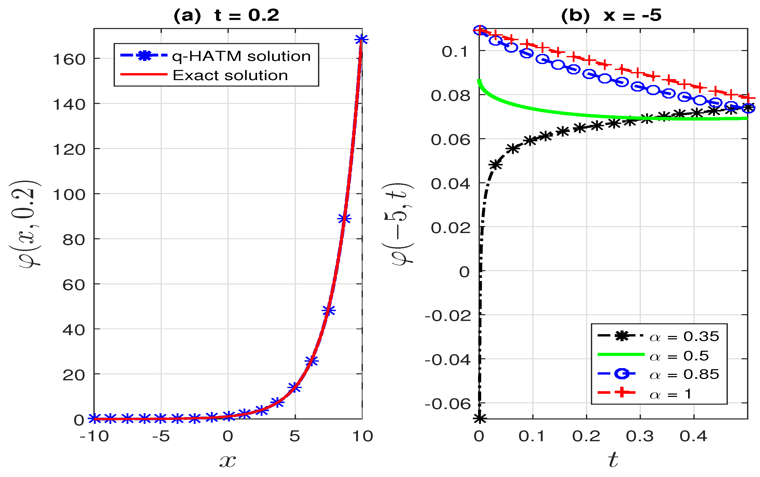
(i) Figure 2 shows the similarity in 3D plot of the exact solution and the solution by the q-HATM for 0 t 1 and 10 x 10 . As can also be seen from Table 1, Figure 4a confirms the closed alignment between the exact solution and the solution by the q-HATM when α = 1 .
(ii) 
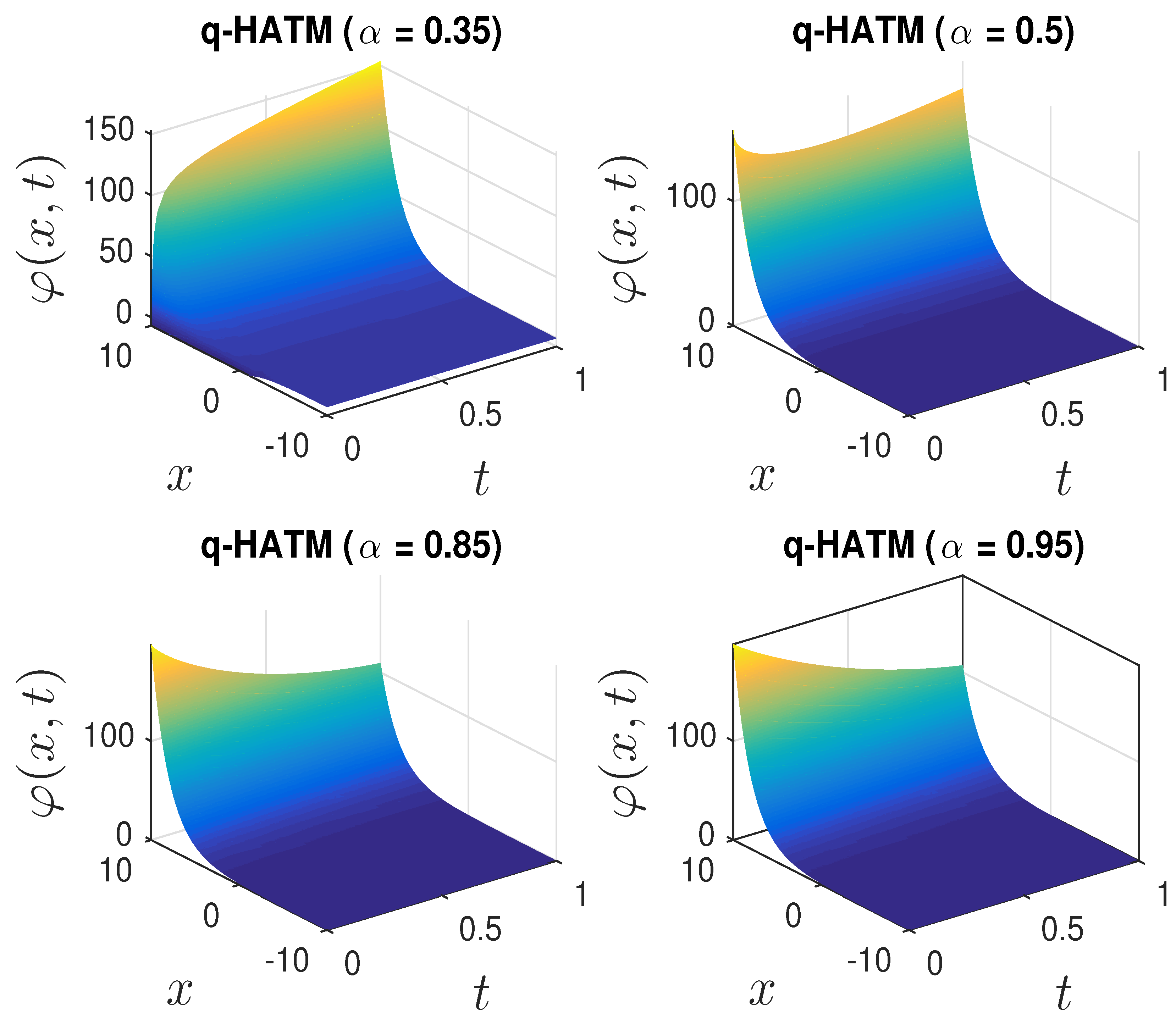
Figure 3 and Figure 4b show the changes in the dynamics of the Fornberg–Whitham equation as the value of α changes. This, in essence, depicts why it is imperative to consider studying the fractional Fornberg–Whitham equation, as this will give additional information about the dynamics of the equation in real life situations.
(iii) 
In Figure 5, with Remark 1 in mind, the ℏ-curve gives the convergence region of the q-HATM solution as 2 < 0 ; then, by means of Figure 1, we make the optimal choice of = 1.28 .
Remark 4. 
Our attention was also drawn to methods presented in other papers—the HAM [48], NIM [51] and NDM (natural transform decomposition method) [50], which were also used to solve the fractional Fornberg–Whitham equation (Equation (2)) with different initial data φ ( x , 0 ) = e x l 2 . We also apply the q-HATM and compare its absolute error with those of the HAM [48], NIM [51] and NDM [50]; see Table 3 below.
Following similar steps leading to Equation (25), for the case where initial data is given as φ ( x , 0 ) = e x / 2 , we obtain the following iterations using the q-HATM:
φ 0 ( x , t ) = e x / 2 φ 1 ( x , t ) = t α e x / 2 2 Γ ( α + 1 ) φ 2 ( x , t ) = 2 t 2 α 1 e x / 2 8 Γ ( 2 α ) + ( 1 + ) t α e x / 2 2 Γ ( α + 1 ) + 2 t 2 α e x / 2 4 Γ ( 2 α + 1 ) .
Using Equation (28), we consider as our approximate solution the sequence of partial sums
φ ( 2 ) ( x , t ) = k = 0 2 φ k ( x , t ) q k .
Thus, taking q = 1 , the approximate solution φ ( 2 ) ( x , t ) of Equation (19) (with φ ( x , 0 ) = e x / 2 ) is
φ ( 2 ) ( x , t ) = e x / 2 + t α e x / 2 2 Γ ( α + 1 ) 2 t 2 α 1 e x / 2 8 Γ ( 2 α ) + ( 1 + ) t α e x / 2 2 Γ ( α + 1 ) + 2 t 2 α e x / 2 4 Γ ( 2 α + 1 ) .
In this case, when φ ( x , 0 ) = e x / 2 , the exact solution to Equation (19) when α = 1 is given as
φ ( x , t ) = e x p x 2 2 t 3 .
This time as well, we also notice from Table 3 that the q-HATM solutions appears to better approximate the exact solution than the other three techniques.

5. Application to a Fractional Biological Population Model

In this section, we are concerned with applying the q-HATM technique to obtain an approximate solution for the following Caputo time-fractional biological population model
D t α φ ( x , y , t ) φ x x 2 ( x , y , t ) φ y y 2 ( x , y , t ) λ φ ( x , y , t ) = 0 , 0 < α 1 , t > 0 ,
with the initial data
φ ( x , y , 0 ) = x y .
The exact solution to Equation (31) when α = 1 is given as
φ ( x , y , t ) = x y e λ t .
We take the Laplace transform (in variable t) of Equation (31) and, due to Equation (32), we get
L t φ 1 s φ ( x , y , 0 ) 1 s α L t 2 φ 2 x 2 + 2 φ 2 y 2 + λ φ = 0 .
Taking ψ ( x , y , t ; q ) , we define the nonlinear function
Υ ( ψ ( x , y , t ; q ) ) = L t ψ 1 s ψ ( x , y , t ; 0 ) 1 s α L t 2 ψ 2 x 2 + 2 ψ 2 y 2 + λ ψ .
From Equation (15), taking H 1 , the kth-order deformation equation is given as
L t φ k η k * φ k 1 = k ( φ k 1 ) ,
where
k ( φ k 1 ) = L t φ k 1 1 η k * 1 s x y λ s α L t φ k 1 2 s α L t j = 0 k 1 φ j 2 φ k 1 j x 2 + j = 0 k 1 φ j x φ k 1 j x 2 s α L t j = 0 k 1 φ j 2 φ k 1 j y 2 + j = 0 k 1 φ j y φ k 1 j y .
Taking the inverse Laplace transform of Equation (35), we get
φ k = η k * φ k 1 + L t 1 k ( φ k 1 ) .
Therefore, making use of Equations (17) and (36) in Equation (37), we obtain the following iterations for the approximate solution:
φ 0 ( x , y , t ) = x y , φ 1 ( x , y , t ) = λ t α x y Γ ( α + 1 ) , φ 2 ( x , y , t ) = ( 1 + ) λ t α x y Γ ( α + 1 ) + 2 λ 2 t 2 α x y Γ ( 2 α + 1 ) .
Using Equation (38), we consider as our approximate solution the sequence of partial sums
φ ( 2 ) ( x , y , t ) = k = 0 2 φ k ( x , y , t ) q k .
Thus, taking q = 1 , the approximate solution φ ( 2 ) ( x , y , t ) of Equation (31) is
φ ( 2 ) ( x , y , t ) = x y λ t α x y Γ ( α + 1 ) λ ( + 1 ) t α x y Γ ( α + 1 ) + λ 2 2 t 2 α x y Γ ( 2 α + 1 ) .

Numerical Comparison

We present in Table 4 the numerical results (when α = 1 ) for t = 1 and some values of x and y. The solutions obtained using the exact solution (Equation (37)), the q-HATM solution (Equation (39)) and absolute errors for the q-HATM and other methods (the LSRPSM [63], the RPSM [63] and the HPM [64]) are tabulated. In Table 4, “itr” means the number of iterations performed for the particular method. In addition, Table 5 shows different numerical result obtained by the q-HATM for different values of α ( α = 0.2 , 0.6 , 0.9 ), with t = 1 , x = 0.3 , 1 and y = 0.1 , 0.2 , 0.3 , 0.4 , 0.5 .
Remark 5. 
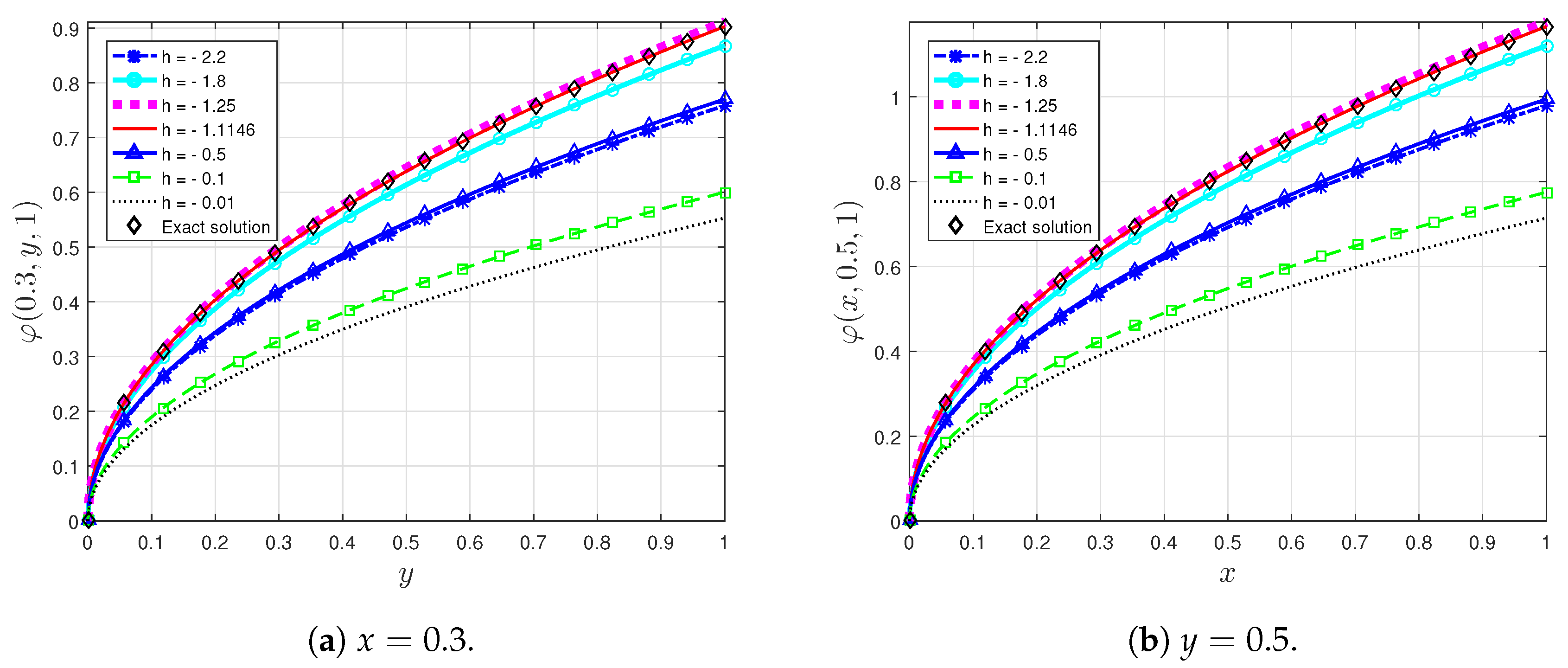
Observe that from Equation (38), we have only performed two iterations of the q-HATM. Moreover, as can be seen from Table 4, when α = 1 and taking = 1.1146 (according to Figure 6), λ = 0.5 , t = 1 , the numerical solution obtained by the q-HATM has a far-reaching match to the exact solution (with smallest absolute error) when compared to other methods presented in the table. Hence, with few iterations, our solution obtained by the q-HATM best approximates the exact solution to a high and appreciable number of significant digits. Moreover, the computations required to obtain our approximate solution φ ( 2 ) ( x , t ) are less strenuous compared to those of the LSRPSM [63], the RPSM [63] and the HPM [64].
Remark 6. 
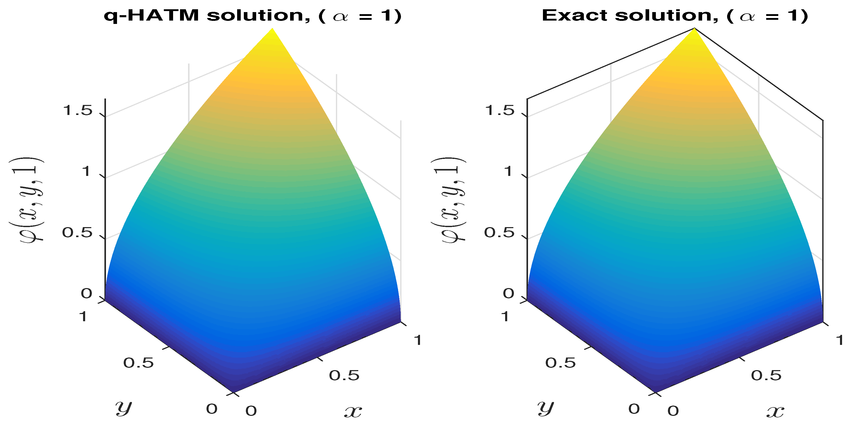
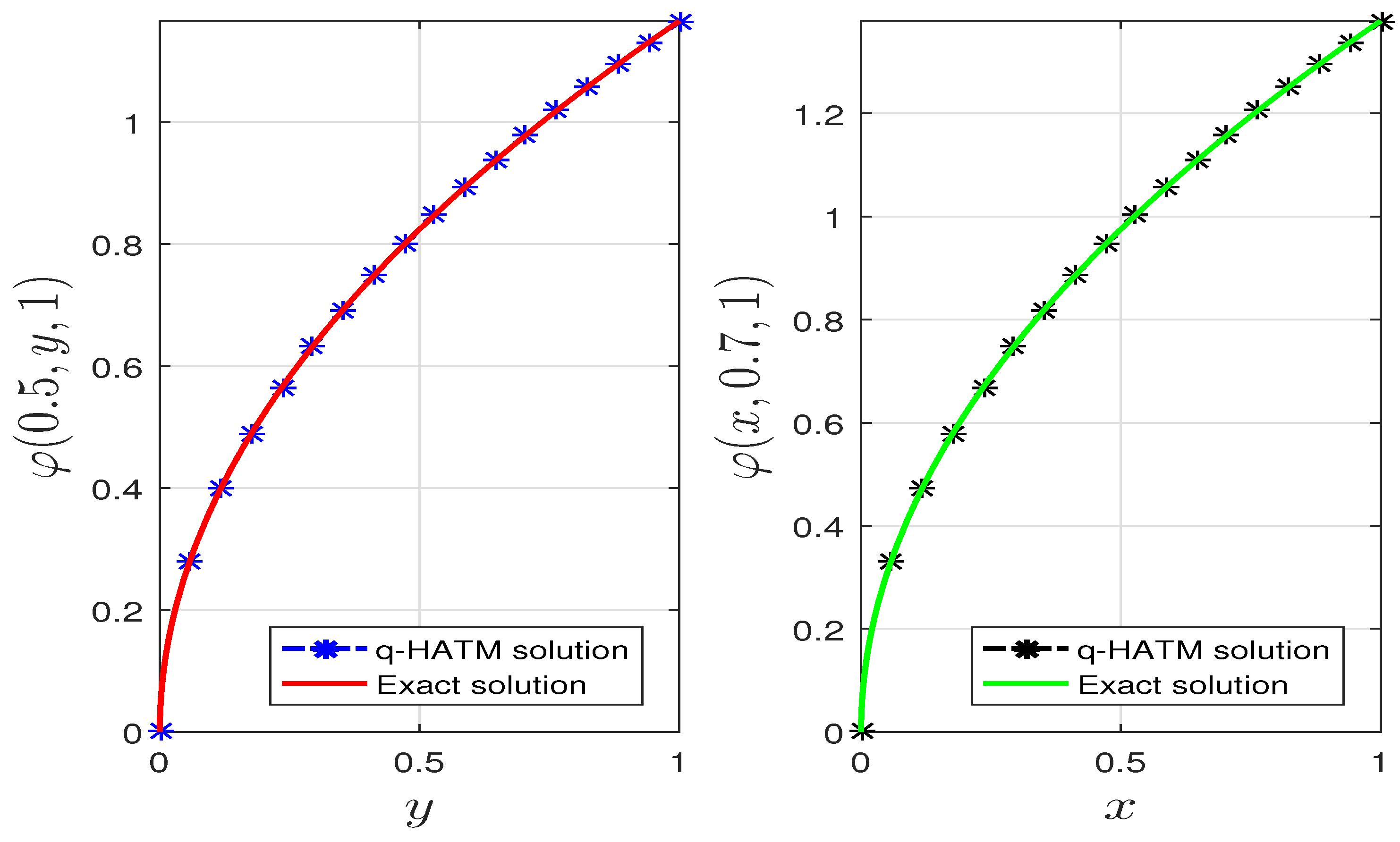
(i) Figure 7 shows the similarity in 3D plot of the exact solution and the solution by the q-HATM for t = 1 , λ = 0.5 , 0 x 1 and 0 y 1 . As can also be seen from Table 4, Figure 8 confirms the closed alignment between the exact solution and the solution by the q-HATM when α = 1 .
(ii) 
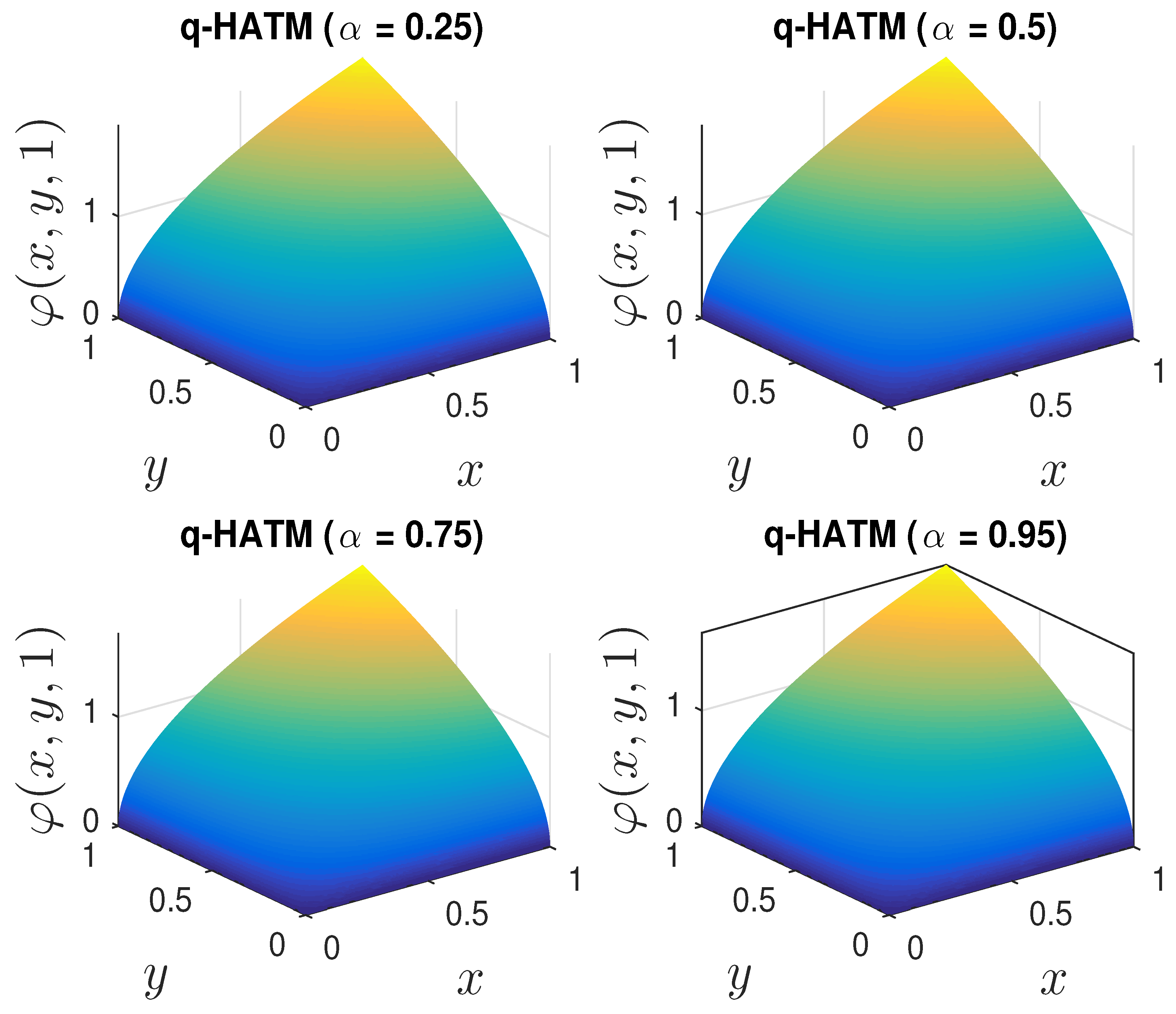
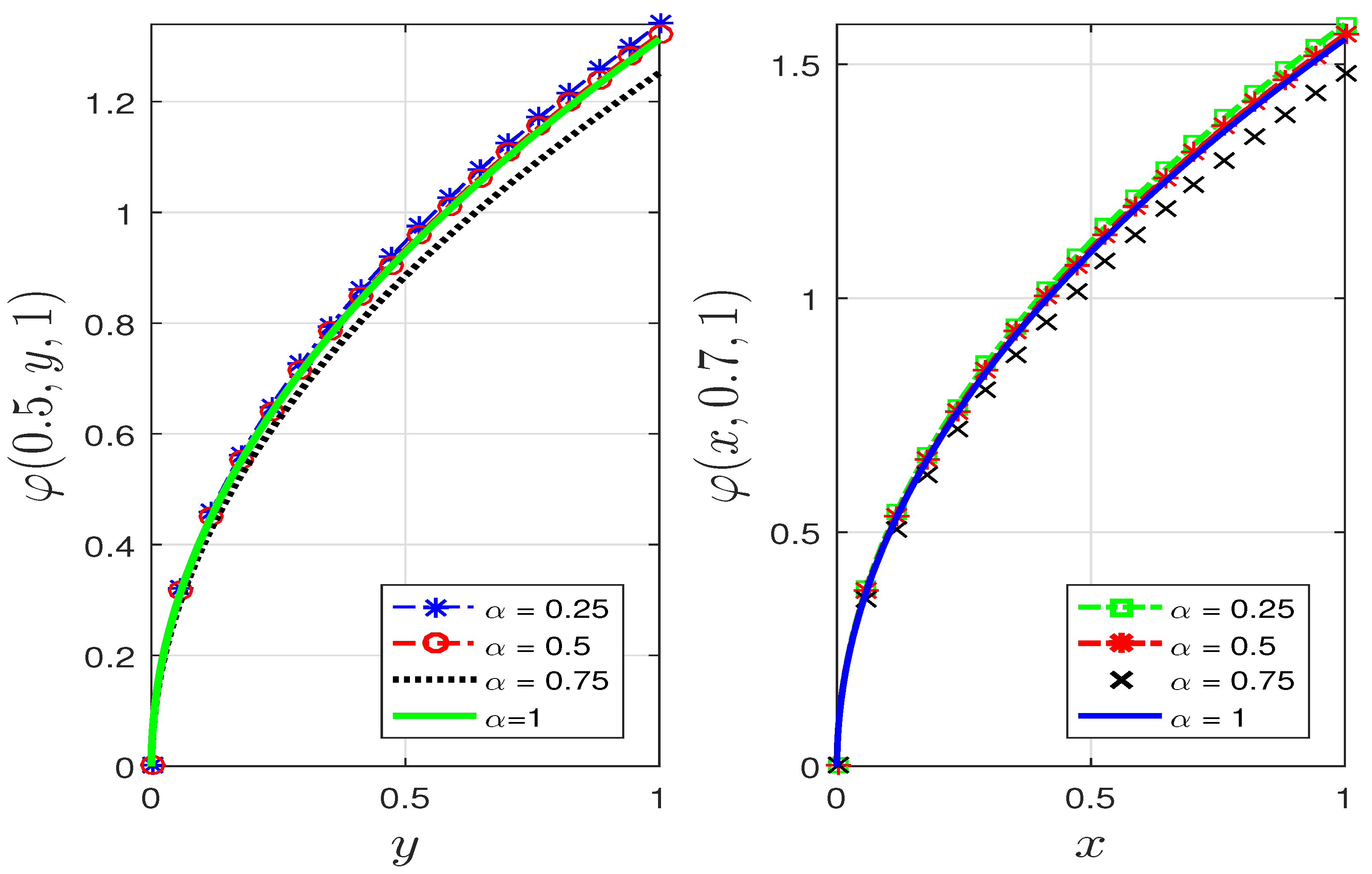
Figure 9 and Figure 10 shows the changes in the dynamics of the fractional biological population Equation (31) as the value of α changes. Thus, the fractional order α gives more information about the dynamics of the biological population model as it relates real life situations.
(iii) 
In Figure 11, in the light of Remark 1, the ℏ-curve gives the convergence region of the q-HATM solution as 2 < 0 ; then, by means of Figure 6, we make the optimal choice of = 1.1146 .

6. Conclusions

In this work, we used the q-homotopy analysis transform method to analyze two Caputo time-fractional differential equations—the Fornberg–Whitham equation and a biological population model. By this method, we were able to obtain approximate solutions for these equations in the form of a series which was obtained from successive iterations. We were able to combine the Laplace transform and the homotopy analysis method (HAM) in an interesting way, and obtained a satisfactory analytical solution of time-fractional nonlinear differential equations both in one space dimension and two space dimensions. Indeed, handling of the nonlinear terms by the applied method was interesting and delicate; perhaps this ensured a better approximate solution as witnessed. From Table 1, Table 3 and Table 4, it is seen that our proposed method performed better than other methods under comparison. In addition, taking advantage of the convergence parameter , only two iterations were sufficient to obtain higher accuracy with our method as against other methods which required more iterations. Comparisons were made between the solution obtained by our proposed method and exact solution, as well as solutions obtained by other methods. This showed that our proposed method converges faster and is more accurate to solve the problems considered in this work. It does appear that our proposed method is quite promising and should be considered to solve other nonlinear differential equations of integer or fractional derivative. In future works, while applying this method, our aim will be to find a better and easier way to obtain the convergence parameter which will guarantee faster convergence and minimum error. One may also consider other methods which also improve on the homotopy series solution, such as the approximate homotopy symmetry method see [39].

Funding

This research received no external funding.

Acknowledgments

The author would like to appreciate the continuous support of University of Hafr Al Batin.

Conflicts of Interest

The author declares no conflict of interest.

References

  1. Debnath, L. A brief historical introduction to fractional calculus. Int. J. Math. Educ. Sci. Technol. 2004, 35, 487–501. [Google Scholar] [CrossRef]
  2. Pu, Y.F. Fractional differential analysis for texture of digital image. J. Algorithms Comput. Technol. 2007, 3, 357–380. [Google Scholar]
  3. Zhang, Y.; Pu, Y.F.; Hu, J.R.; Zhou, J.L. A class of fractional-order variational image in-painting models. Appl. Math. Inf. Sci. 2012, 6, 299–306. [Google Scholar]
  4. Kumar, D.; Seadawy, A.R.; Joardar, A.K. Modified Kudryashov method via new exact solutions for some conformable fractional differential equations arising in mathematical biology. Chin. J. Phys. 2018, 56, 75–85. [Google Scholar] [CrossRef]
  5. Baleanu, D.; Guvenc, Z.B.; Machado, J.T. New Trends in Nanotechnology and Fractional Calculus Applications; Springer: Berlin/Heidelberg, Germany, 2010. [Google Scholar]
  6. Mainardi, F. Fractional Calculus and Waves in Linear Viscoelasticity; Imperial College Press: London, UK, 2010. [Google Scholar]
  7. Agarwal, P.; Dragomir, S.S.; Jleli, M.; Samet, B. Advances in Mathematical Inequalities and Applications; Springer: Berlin/Heidelberg, Germany, 2018. [Google Scholar]
  8. Baleanu, D.; Jajarmi, A.; Sajjadi, S.S.; Mozyrska, D. A new fractional model and optimal control of a tumor-immune surveillance with non-singular derivative operator. Chaos Interdiscip. J. Nonlinear Sci. 2019, 29, 083127. [Google Scholar] [CrossRef]
  9. El-Sayed, A.A.; Agarwal, P. Numerical solution of multiterm variable order fractional differential equations via shifted Legendre polynomials. Math. Methods Appl. Sci. 2019, 42, 3978–3991. [Google Scholar] [CrossRef]
  10. El-Tawil, M.A.; Huseen, S.N. The Q-homotopy analysis method (QHAM). Int. J. Appl. Math. Mech. 2012, 8, 51–75. [Google Scholar]
  11. Fornberg, B.; Whitham, G.B. A numerical and theoretical study of certain nonlinear wave phenomena. Philos. Trans. R. Soc. Lond. Ser. A Math. Phys. Sci. 1978, 298, 373–404. [Google Scholar]
  12. Iyiola, O.S. A numerical study of Ito equation and Sawada–Kotera equation both of time-fractional type. Adv. Math. Sci. J. 2013, 2, 71–79. [Google Scholar]
  13. Iyiola, O.S. On the solutions of non-linear time-fractional gas dynamic equations: An analytical approach. Int. J. Pure Appl. Math. 2015, 98, 491–502. [Google Scholar] [CrossRef] [Green Version]
  14. Iyiola, O.S.; Soh, M.E.; Enyi, C.D. Generalised homotopy analysis method (q-HAM) for solving foam drainage equation of time fractional type. Math. Eng. Sci. Aerosp. 2013, 4, 105. [Google Scholar]
  15. Jain, S.; Agarwal, P.; Kilicman, A. Pathway fractional integral operator associated with 3m-parametric Mittag-Leffler functions. Int. J. Appl. Comput. Math. 2018, 4, 115. [Google Scholar] [CrossRef]
  16. Jain, S.; Mehrez, K.; Baleanu, D.; Agarwal, P. Certain Hermite–Hadamard inequalities for logarithmically convex functions with applications. Mathematics 2019, 7, 163. [Google Scholar] [CrossRef] [Green Version]
  17. Jajarmi, A.; Arshad, S.; Baleanu, D. A new fractional modelling and control strategy for the outbreak of dengue fever. Phys. A Stat. Mech. Appl. 2019, 535, 122524. [Google Scholar] [CrossRef]
  18. Jajarmi, A.; Baleanu, D.; Sajjadi, S.S.; Asad, J.H. A new feature of the fractional Euler–Lagrange equations for a coupled oscillator using a nonsingular operator approach. Front. Phys. 2019, 7, 196. [Google Scholar] [CrossRef] [Green Version]
  19. Jajarmi, A.; Ghanbari, B.; Baleanu, D. A new and efficient numerical method for the fractional modelling and optimal control of diabetes and tuberculosis co-existence. Chaos Interdiscip. J. Nonlinear Sci. 2019, 29, 093111. [Google Scholar] [CrossRef] [PubMed]
  20. Jajarmi, A.; Yusuf, A.; Baleanu, D.; Inc, M. A new fractional HRSV model and its optimal control: A non-singular operator approach. Phys. A Stat. Mech. Appl. 2020, 547, 123860. [Google Scholar] [CrossRef]
  21. Nigmatullina, R.R.; Agarwal, P. Direct evaluation of the desired correlations: Verification on real data. Phys. A Stat. Mech. Appl. 2019, 534, 121558. [Google Scholar] [CrossRef]
  22. Qureshi, S.; Yusuf, A. Fractional derivatives applied to MSEIR problems: Comparative study with real world data. Eur. Phys. J. Plus 2019, 134, 171. [Google Scholar] [CrossRef]
  23. Qureshi, S.; Yusuf, A. Mathematical modeling for the impacts of deforestation on wildlife species using Caputo differential operator. Chaos Solitons Fractals 2019, 126, 32–40. [Google Scholar] [CrossRef]
  24. Rekhviashvili, S.; Pskhu, A.; Agarwal, P.; Jain, S. Application of the fractional oscillator model to describe damped vibrations. Turk. J. Phys. 2019, 43, 236–242. [Google Scholar] [CrossRef]
  25. Ruzhansky, M.V.; Cho, Y.J.; Agarwal, P.; Area, I. Advances in Real and Complex Analysis with Applications; Springer: Singapore, 2017. [Google Scholar]
  26. Sakar, M.G.; Erdogan, F.; Yildirim, A. Variational iteration method for the time-fractional Fornberg-Whitham equation. Compt. Math. Appl. 2012, 63, 1382–1388. [Google Scholar] [CrossRef] [Green Version]
  27. Saoudi, K.; Agarwal, P.; Kumam, P.; Ghanmi, A.; Thounthong, P. The Nehari manifold for a boundary value problem involving Riemann–Liouville fractional derivative. Adv. Differ. Equ. 2018, 2018, 263. [Google Scholar] [CrossRef] [Green Version]
  28. Senol, M.; Iyiola, O.S.; Kasmaei, H.D.; Akinyemi, L. Efficient analytical techniques for solving time-fractional nonlinear coupled Jaulent–Miodek system with energy-dependent Schrödinger potential. Adv. Differ. Equ. 2019, 2019, 462. [Google Scholar] [CrossRef]
  29. Singh, J.; Kumar, D.; Kumar, S. New treatment of fractional Fornberg-Whitham equation via Laplace transform. Ain Shams Eng. J. 2013, 4, 557–562. [Google Scholar] [CrossRef] [Green Version]
  30. Singh, J.; Kumar, D.; Swroop, R. Numerical solution of time and space-fractional coupled Burgers’ equations via homotopy algorithm. Alex. Eng. J. 2016, 55, 1753–1763. [Google Scholar] [CrossRef] [Green Version]
  31. Singh, J.; Kumar, D.; Baleanu, D.; Rathore, S. An efficient numerical algorithm for the fractional Drinfeld–Sokolov–Wilson equation. Appl. Math. Comput. 2018, 335, 12–24. [Google Scholar] [CrossRef]
  32. Soh, M.E.; Enyi, C.D.; Iyiola, O.S.; Audu, J.D. Approximate analytical solutions of strongly nonlinear fractional BBM-Burger’s equations with dissipative term. Appl. Math. Sci. 2014, 8, 7715–7726. [Google Scholar] [CrossRef] [Green Version]
  33. Srivastava, H.M.; Kumar, D.; Singh, J. An efficient analytical technique for fractional model of vibration equation. Appl. Math. Model. 2017, 45, 192–204. [Google Scholar] [CrossRef]
  34. Veeresha, P.; Prakasha, D.G.; Qurashi, M.A.; Baleanu, D. A reliable technique for fractional modified Boussinesq and approximate long wave equations. Adv. Differ. Equ. 2019, 2019, 253. [Google Scholar] [CrossRef]
  35. Niu, Z.; Wang, C. A one-step optimal homotopy analysis method for nonlinear differential equations. Commun. Nonlinear Sci. Numer. Simul. 2010, 15, 2026–2036. [Google Scholar] [CrossRef]
  36. Whitham, G.B. Variational methods and applications to water waves. Philos. Trans. R. Soc. Lond. Ser. A Math. Phys. Sci. 1967, 299, 6–25. [Google Scholar]
  37. Yabushita, K.; Yamashita, M.; Tsuboi, K. An analytic solution of projectile motion with the quadratic resistance law using the homotopy analysis method. J. Phys. A Math. Theor. 2007, 40, 8403–8416. [Google Scholar] [CrossRef]
  38. Yıldız, T.A.; Jajarmi, A.; Yıldız, B.; Baleanu, D. New aspects of time fractional optimal control problems within operators with nonsingular kernel. Discrete Contin. Dyn. Syst. 2020, 13, 407–428. [Google Scholar] [CrossRef] [Green Version]
  39. Yu, J.X.; Yuan, G.; Yua, L.S. Approximate homotopy symmetry method: Homotopy series solutions to the sixth-order Boussinesq equation. Sci. China Ser. G-Phys. Mech. Astron. 2009, 52, 1169–1178. [Google Scholar]
  40. Yusuf, A.; Qureshi, S.; Shah, S.F. Mathematical analysis for an autonomous financial dynamical system via classical and modern fractional operators. Chaos Solitons Fractals 2020, 132, 109552. [Google Scholar] [CrossRef]
  41. Liao, S.J. Homotopy analysis method and its applications in mathematics. J. Basic Sci. Eng. 1997, 5, 111–125. [Google Scholar]
  42. Liao, S.J. Homotopy analysis method: A new analytic method for nonlinear problems. Appl. Math. Mech. 1998, 19, 957–962. [Google Scholar]
  43. Akinyemi, L. q-homotopy analysis method for solving the seventh-order time-fractional Lax’s Korteweg–de Vries and Sawada–Kotera equations. Comput. Appl. Math. 2019, 38, 191. [Google Scholar] [CrossRef]
  44. Akinyemi, L.; Iyiola, O.S.; Akpan, U. Iterative methods for solving fourth- and sixth-order time-fractional Cahn–Hillard equation. Math. Methods Appl. Sci. 2020, 43, 4050–4074. [Google Scholar] [CrossRef] [Green Version]
  45. Kumar, D.; Agarwal, R.P.; Singh, J. A modified numerical scheme and convergence analysis for fractional model of Lienard’s equation. J. Comput. Appl. Math. 2018, 399, 405–413. [Google Scholar] [CrossRef]
  46. Kumar, D.; Singha, J.; Baleanu, D. A new analysis for fractional model of regularized long-wave equation arising in ion acoustic plasma waves. Math. Methods Appl. Sci. 2017, 40, 5642–5653. [Google Scholar] [CrossRef]
  47. Prakash, A.; Veeresha, P.; Prakasha, D.G.; Goyal, M. A homotopy technique for fractional order multi-dimensional telegraph equation via Laplace transform. Eur. Phys. J. Plus 2019, 134, 19. [Google Scholar] [CrossRef]
  48. Abidi, F.; Omrani, K. The homotopy analysis method for solving the Fornberg-Whitham equation and comparison with the Adomian’s decomposition method. Comp. Maths. Appl. 2010, 59, 2743–2750. [Google Scholar] [CrossRef] [Green Version]
  49. Lu, J. An analytical approach to the Fornberg-Whitham type equations by using variational iteration method. Comp. Maths. Appl. 2011, 61, 2010–2013. [Google Scholar] [CrossRef] [Green Version]
  50. Alderremy, A.A.; Khan, H.; Shah, R.; Aly, S.; Baleanu, D. The analytical analysis of time-fractional Fornberg—Whitham equations. Mathematics 2020, 8, 987. [Google Scholar] [CrossRef]
  51. Al-luhaibi, M.S. An analytical treatment to fractional Fornberg—Whitham equation. Math Sci. 2017, 11, 1–6. [Google Scholar] [CrossRef] [Green Version]
  52. Kumar, D.; Singh, J.; Baleanu, D. A new analysis of the Fornberg-Whitham equation pertaining to a fractional derivative with Mittag-Leffler-type kernel. Eur. Phys. J. Plus 2018, 133, 70. [Google Scholar] [CrossRef]
  53. Merdan, M.; Gökdoğan, A.; Yıldırım, A.; Mohyud-Din, S.T. Numerical simulation of fractional Fornberg-Whitham equation by differential transformation method. Abstract Appl. Anal. 2012, 2012, 965367. [Google Scholar] [CrossRef]
  54. Akinyemi, L.; Iyiola, O.S.; Akpan, U. A reliable technique to study nonlinear time-fractional coupled Korteweg—de Vries equations. Adv. Difference Equ. 2020, 2020, 169. [Google Scholar] [CrossRef] [Green Version]
  55. Kilbas, A.A.; Srivastava, H.M.; Trujillo, J.J. Theory and Applications of Fractional Differential Equations; Elsevier: Amsterdam, The Netherlands, 2006. [Google Scholar]
  56. Luchko, Y.F.; Srivastava, H.M. The exact solution of certain differential equations of fractional order by using operational calculus. Comput. Math. Appl. 1995, 29, 73–85. [Google Scholar] [CrossRef] [Green Version]
  57. Podlubny, I. Fractional Differential Equations; Academic Press: New York, NY, USA, 1999. [Google Scholar]
  58. Caputo, M. Elasticita e Dissipazione; Zanichelli: Bologna, Italy, 1969. [Google Scholar]
  59. Odibat, Z.M.; Shawagfeh, N.T. Generalized Taylor’s formula. Appl. Math. Comput. 2007, 186, 286–293. [Google Scholar] [CrossRef]
  60. Argyros, I.K. Convergence and Applications of Newton-Type Iterations; Springer: New York, NY, USA, 2008. [Google Scholar]
  61. Abbasbandy, S.; Jalili, M. Determination of optimal convergence-control parameter value in homotopy analysis method. Numer. Algor. 2013, 64, 593–605. [Google Scholar] [CrossRef]
  62. Liao, S.J. The Homotopy Analysis Method in Nonlinear Differential Equations; Higher Education Press: Beijing, China; Springer: Berlin/Heidelberg, Germany, 2012. [Google Scholar]
  63. Zhang, J.; Wei, Z.; Li, L.; Zhou, C. Least-squares residual power series method for the time fractional differential equations. Complexity 2019, 2019, 6159024. [Google Scholar] [CrossRef]
  64. Liu, Y.; Li, Z.; Zhang, Y. Homotopy perturbation method to fractional biological population equation. Diff. Calculus. 2011, 1, 117–127. [Google Scholar] [CrossRef]
Figure 1. Plots of the q-HATM solutions for different -values and exact solution for α = 1 .
Symmetry 12 01976 g001
Figure 2. 3D plot of the exact solution and the q-HATM solution, with α = 1 , = 1.28 .
Symmetry 12 01976 g002
Figure 3. 3D plot of the q-HATM solution with different α values and = 1.28 .
Symmetry 12 01976 g003
Figure 4. (a) is the line plot of the exact and q-HATM solutions when α = 1 at fixed t = 0.2 and = 1.28 . (b) shows the effect of different values of α for fixed x = 5 and = 1.28 .
Symmetry 12 01976 g004
Figure 5. -curve plots for different values of α .
Symmetry 12 01976 g005
Figure 6. Plots of the q-HATM solutions for different -values and exact solution, for α = 1 and t = 1 .
Symmetry 12 01976 g006
Figure 7. 3D plot of the exact solution and the q-HATM solution, with α = 1 , = 1.1146 , λ = 0.5 , t = 1 .
Symmetry 12 01976 g007
Figure 8. Line plot of the exact and q-HATM solutions with = 1.1146 when α = 1 , t = 1 , λ = 0.5 and for fixed x = 0.5 (left) and fixed y = 0.7 (right).
Symmetry 12 01976 g008
Figure 9. 3D plot of the q-HATM solution for different α values, with = 1.1146 , λ = 0.5 , t = 1 .
Symmetry 12 01976 g009
Figure 10. Effects of different values of α for t = 1 , λ = 0.5 , = 1.1146 and for fixed x = 0.5 (left) and fixed y = 0.7 (right).
Symmetry 12 01976 g010
Figure 11. -curve plots for different values of α .
Symmetry 12 01976 g011
Table 1. Numerical comparison when α = 1 of the exact solution (Equation (21)), and the solutions obtained by the q-homotopy analysis transform method (q-HATM) with = 1.28 , the least-squares residual power series method (LSRPSM) [63], the residual power series method (RPSM) [63] and the variational iteration method (VIM) [26].
φ ( x , t ) φ ( 2 ) ( x , t ) Abs ErrorAbs ErrorAbs ErrorAbs Error
xtExactq-HATMq-HATMLSRPSM [63]RPSM [63]VIM [26]
itr = 2itr = 2itr = 2itr = 5itr = 2
0.10.008404530.008404361.70560 × 10 7 1.21387 × 10 5 1.41249 × 10 4 1.75478 × 10 2
10 0.20.007862500.007861599.10243 × 10 7 1.58400 × 10 5 1.58400 × 10 5 1.71128 × 10 2
0.30.007355420.007355611.90881 × 10 7 1.35139 × 10 5 3.77120 × 10 4 1.66654 × 10 2
0.40.006881050.006886435.38732 × 10 6 7.41498 × 10 6 4.74372 × 10 4 1.62077 × 10 2
0.50.006437270.006454051.67882 × 10 5 3.47756 × 10 7 5.59422 × 10 4 1.57418 × 10 2
0.10.102388120.102386042.07785 × 10 6 1.47879 × 10 4 1.72077 × 10 3 2.13776 × 10 1
5 0.20.095784800.095773711.10890 × 10 5 1.92971 × 10 4 3.24664 × 10 3 2.08477 × 10 1
0.30.089607350.089609682.32540 × 10 6 1.64633 × 10 4 4.59427 × 10 3 2.03026 × 10 1
0.40.083828300.083893936.56310 × 10 5 9.03330 × 10 5 5.77904 × 10 3 1.97450 × 10 1
0.50.078421960.078626482.04522 × 10 4 4.23654 × 10 6 6.81515 × 10 3 1.91774 × 10 1
0.12.056520352.056478624.17347 × 10 5 2.97023 × 10 3 3.45626 × 10 2 4.29380
10.21.923889161.923666432.22729 × 10 4 3.87592 × 10 3 6.52104 × 10 2 4.18737
0.31.799811741.799858454.67070 × 10 5 3.30675 × 10 3 9.22783 × 10 2 4.07788
0.41.683736461.685054691.31823 × 10 3 1.81439 × 10 3 1.16075 × 10 1 3.96588
0.51.575147221.579255154.10793 × 10 3 8.50920 × 10 5 1.36886 × 10 1 3.85189
Table 2. Values of the approximate solution φ ( 2 ) ( x , t ) by the q-HATM, for different values of α .
xt α = 0.25 α = 0.5 α = 0.75
0.10.054163160.073519170.09275676
0.20.066581850.070548020.08474062
−50.30.072885530.069311230.07889088
0.40.077194280.068972220.07438139
0.50.080542780.069206930.07085670
0.18.0385263310.9112120813.76632402
0.29.8816229710.4702542912.57662352
50.310.8171711510.2866990211.70844537
0.411.4566467610.2363851011.03917664
0.511.9536085210.2712197510.51606638
Table 3. Numerical comparison when α = 1 of the exact solution (Equation (21)) (with φ ( x , 0 ) = e x / 2 ), and the solutions obtained by the q-HATM with = 1.26 , the homotopy analysis method (HAM) [48], the new iteration method (NIM) [51] and the natural transform decomposition method (NDM) [50].
φ ( x , t ) φ ( 2 ) ( x , t ) Abs ErrorAbs ErrorAbs ErrorAbs Error
xtExactq-HATMq-HATMHAM [48]NIM [51]NDM [50]
itr = 2itr = 2itr = 5itr = 3itr = 3
0.10.006303400.006303488.43252 × 10 8 1.25020 × 10 4 9.90107 × 10 5 4.86602 × 10 6
0.20.005896870.005895761.11391 × 10 6 5.33187 × 10 4 1.84777 × 10 4 6.13163 × 10 6
10 0.30.005516560.005514781.78726 × 10 6 1.22446 × 10 3 2.56333 × 10 4 4.76202 × 10 6
0.40.005160780.005160542.44846 × 10 7 2.19875 × 10 3 3.12832 × 10 4 1.60584 × 10 6
0.50.004827950.004833055.09516 × 10 6 3.45598 × 10 3 3.53532 × 10 4 2.59733 × 10 6
0.10.076791090.076792121.02729 × 10 6 1.52306 × 10 3 1.20620 × 10 3 5.92803 × 10 5
0.20.071838600.071825031.35702 × 10 5 6.49555 × 10 3 2.25104 × 10 3 7.46985 × 10 5
5 0.30.067205510.067183742.17733 × 10 5 1.49169 × 10 2 3.12278 × 10 3 5.80133 × 10 5
0.40.062871230.062868242.98283 × 10 6 2.67863 × 10 2 3.81107 × 10 3 1.95632 × 10 5
0.50.058816470.058878546.20718 × 10 5 4.21025 × 10 2 4.30690 × 10 3 3.16419 × 10 5
0.11.542390271.542410902.06337 × 10 5 3.05915 × 10 2 2.42271 × 10 2 1.19068 × 10 3
0.21.442916871.442644302.72565 × 10 4 1.30467 × 10 1 4.52134 × 10 2 1.50036 × 10 3
10.31.349858811.349421484.37328 × 10 4 2.99615 × 10 1 6.27227 × 10 2 1.16523 × 10 3
0.41.262802341.262742435.99118 × 10 5 5.38018 × 10 1 7.65474 × 10 2 3.92937 × 10 4
0.51.181360411.182607161.24675 × 10 3 8.45651 × 10 1 8.65064 × 10 2 6.35545 × 10 4
Table 4. Numerical comparison when α = 1 of the exact solution (Equation (21)), and the solutions obtained by the q-HATM with = 1.1146 , the LSRPSM [63], the RPSM [63] and the homotopy perturbation method (HPM) [64]. We take t = 1 , λ = 0.5 .
φ ( x , y , t ) φ ( 2 ) ( x , y , t ) Abs ErrorAbs ErrorAbs ErrorAbs Error
xyExactq-HATMq-HATMLSRPSM [63]RPSM [63]HPM [64]
itr = 2itr = 2itr = 2itr = 2itr = 2
0.10.164872130.164872513.7943 × 10 7 9.62 × 10 6 2.37 × 10 3 2.3721 × 10 3
0.20.233164400.233164935.3660 × 10 7 1.36 × 10 5 3.35 × 10 3 3.3547 × 10 3
0.10.30.285566900.285567566.5719 × 10 7 1.67 × 10 5 4.11 × 10 3 4.1086 × 10 3
0.40.329744250.329745017.5886 × 10 7 1.92 × 10 5 4.74 × 10 3 4.7443 × 10 3
0.50.368665280.368666138.4843 × 10 7 2.15 × 10 5 5.30 × 10 3 5.3042 × 10 3
0.10.285566900.285567566.5719 × 10 7 1.67 × 10 5 4.11 × 10 3 4.1086 × 10 3
0.20.403852580.403853519.2941 × 10 7 2.36 × 10 5 5.81 × 10 3 5.8105 × 10 3
0.30.30.494616380.494617521.1383 × 10 6 2.89 × 10 5 7.12 × 10 3 7.1164 × 10 3
0.40.571133800.571135121.3144 × 10 6 3.33 × 10 5 8.22 × 10 3 8.2173 × 10 3
0.50.638547000.638548471.4695 × 10 6 3.73 × 10 5 9.19 × 10 3 9.1872 × 10 3
0.10.368665280.368666138.4843 × 10 7 2.15 × 10 5 5.30 × 10 3 5.3042 × 10 3
0.20.521371440.521372641.1999 × 10 6 3.04 × 10 5 7.50 × 10 3 7.5013 × 10 3
0.50.30.638547000.638548471.4695 × 10 6 3.73 × 10 5 9.19 × 10 3 9.1872 × 10 3
0.40.737330570.737332261.6969 × 10 6 4.30 × 10 5 1.06 × 10 2 1.0608 × 10 2
0.50.824360640.824362531.8971 × 10 6 4.81 × 10 5 1.19 × 10 2 1.1861 × 10 2
0.10.521371440.521372641.1999 × 10 6 3.04 × 10 5 7.50 × 10 3 7.5013 × 10 3
0.20.737330570.737332261.6969 × 10 6 4.30 × 10 5 1.06 × 10 2 1.0608 × 10 2
1.00.30.903041830.903043912.0782 × 10 6 5.27 × 10 5 1.30 × 10 2 1.2993 × 10 2
0.41.042742891.042745292.3997 × 10 6 6.09 × 10 5 1.50 × 10 2 1.5003 × 10 2
0.51.165821991.165824672.6830 × 10 6 6.80 × 10 5 1.68 × 10 2 1.6773 × 10 2
Table 5. Values of the approximate solution φ ( 2 ) ( x , t ) by the q-HATM for different values of α , when t = 1 .
xy α = 0.2 α = 0.6 α = 0.9
0.10.326917060.317679750.29415547
0.20.462330540.449267000.41599866
0.30.30.566236960.550237460.50949222
0.40.653834130.635359490.58831095
0.50.731008780.710353510.65775163
0.10.596866170.410122790.53705196
0.20.844096230.580001210.75950617
10.31.033802530.710353510.93020128
0.41.193732330.820245571.07410392
0.51.334633320.917062431.20088469
Publisher’s Note: MDPI stays neutral with regard to jurisdictional claims in published maps and institutional affiliations.