The Design of GLR Control Chart for Monitoring the Geometric Observations Using Sequential Sampling Scheme

Abstract

The control charts’ design is focused on system forecasting which is important in mathematics and statistics; these techniques are commonly employed in manufacturing industries. The need for a control chart that can conceptualize and identify the symmetric or asymmetric structure of the monitoring phase with more than one aspect of the standard attribute is a necessity of industries. The generalized likelihood ratio (GLR) chart is a well-known method to track both the decrease and increase in the mechanism effectively. A control chart, termed as a GLR control chart, is established in this article, focusing on a sequential sampling scheme (the SS GLR chart) to evaluate the geometrically distributed process parameter. The SS GLR chart statistic is examined on a window of past samples. In contexts of the steady-state average time to signal, the output of the SS GLR control chart is analyzed and compared with the non-sequential geometric GLR chart and the cumulative sum (CUSUM) charts. In this article, the optimum parameter options are presented, and regression equations are established to calculate the SS GLR chart limits.

1. Introduction

Statistical process control charts are powerful visual techniques for monitoring the process’s cohesion and investigating how it modifies over time. In the general scheme of measures taken to regulate mass production efficiency, the techniques of statistical quality control perform a significant part. This is mainly due to the assumption that the uncertainty of the mathematical features of the fundamental consistency metrics is unpredictable by nature. Attempts to keep the monitoring more transparent and devoid of systemic errors make it possible to use replication approaches, which in exchange, making it imperative to utilize probabilistic and predictive methodologies. The industries appear to be highly dependent on the control charts approaches and advancements to sustain business in the challenging sector across the globe. The variation towards the industrial process’s goal can be identified by the statistical significance of the statistics [1]. The control charts of the Shewhart method, proposed in Shewhart (1931) [2], are accurate in identifying wide variations. Through comparison, the exponentially weighted moving average (EWMA) and the cumulative sum (CUSUM) charts have become accurate in identifying small shifts in control factors domains. In general, a control chart can be constructed as per the desired in-control average run length (ARL₀), including susceptibility for capturing the parameter changes in an out-of-control situation.

One approach to achieve successful results throughout the varied variety of shift ranges is combining dual or further control charts. A Shewhart chart, for instance, can be utilized in connection with a CUSUM chart, for which the Shewhart chart can efficiently identify massive changes, as well as the CUSUM chart is able to quickly detect tiny shifts (check, for reference, Westgard et al. (1977), Wu et al. (2008)) [3,4]. Of course, the Shewhart chart is a unique case of the CUSUM chart, while this method probably uses two CUSUM charts.

Combining multiple CUSUM charts is a core component of such a notion. Lorden (1971) [5] initially examined the use of multiple CUSUM charts, and some studies comprise, Sparks (2000), Zhao, et al. (2005), and Han et al. (2007) [6,7,8]. The main drawback of exercising numerous charts is that developing such a structure demands that for various charts, the control charts’ parameters need to be defined.

The negative distribution of binomials was debated by Jackson (1972) [9], as one interim solution to the Poisson distribution. This approach has also been examined by Sheaffer and Leavenworth (1976) [10], who moreover, studied the approximate confidence intervals and control charts for the negative binomial. Bourke (1991) [11] utilized negative binomial distribution to identify the run length of the manufacturing cycle in successive discrepancies.

Geometric distribution defines the number of Bernoulli experiments required to alter the situation in a discrete phase [12]. On the other hand, the exponential distribution distinguishes the time to change status in a continuous phase. One can choose control charts centered on geometric and exponential distribution statistics to track numbers amongst rare occurrences or unfavorable outcomes besides interval among exceptional trials.

For instance, a control chart formulated by Benneyan (2001) [13] for tracking unfavorable outcomes (geometric distribution) amongst g-type control charts, while a control chart focused on exponential distribution developed by Santiago and Smith (2013) [14]. The geometric control chart has shown quite efficiently tracking the nonconforming proportions of high-quality procedures compared to Shewhart $np$ or $p$ charts. For yes/no kind attribute results, p and np control charts are being used. These two charts are widely used in a subgroup of resources to track the fraction (p chart) or number (np chart) of faulty items. [15]. Executing a geometric chart usually includes the assertion that the nonconforming in-control ratio is defined or measured adequately. The number of corresponding entries among two succeeding nonconforming items is utilized in the geometric model to regulate the mechanism. Therefore, the geometric chart does not entail aggregating historical data (Kim and Lee) (2015) [16].

Chang and Gan (2001) [17] presented a CUSUM chart for parameter examining in high-yield procedures. They did not follow the renovation approach since they assumed that a transformation of the geometric distribution to a nearly normal distribution is available to model control charts. However, it could be challenging to perceive the altered statistics for control charts; (check for reference Xie et al. (1995), Quesenberry (1995), and Kaminsky et al. (1992)) [18,19,20].

The particular drawback of exercising the conventional Shewhart, EWMA, or CUSUM charts for process examining is that such charts are considered to acquire quick recognition across the alteration size. They are modified to identify but are not efficient in case the actual alteration is extremely faraway from whatever is predicted. Another choice for significantly boosted functioning in handling a broad variety of changes is to practice a control chart relying on a statistic of a generalized likelihood ratio (GLR) chart. GLR control charts have already been designed for several cases, functioning as measuring the variance as well as the mean of a normal process. The vector constraint in multinomial function and the ratio of uncommon products in Bernoulli and binomial procedures. For detailed information, refer to Willsky and Jones (1976), Siegmund and Venkatraman (1995), Hawkins and Zamba (2005), Lai and Shan (1999), Reynolds and Lou (2010, 2012), and Hung et al. (2012, 2013), and Lee et al. (2017), [21,22,23,24,25,26,27,28].

GLR control charts often have the additional benefit that in evaluating the GLR statistics, measurements of the system change-point and alteration size are given, which are sufficient for post-signal analysis. Huang et al. [27] analyzed a GLR chart focused on the binomial distribution to detect boosts in p in the situation where samples of size n > 1 are drawn from the procedure, where p is the probability of success on an individual trial and n is the sample size.

When implementing a control chart in-process, examining the sample at a fixed sampling rate (FSR) is the standard approach. Exercising a fixed sampling interval (FSI) amongst trials, an FSR control chart takes samples at a fixed sample size (FSS). FSR control charts’ efficiency may be enhanced by changing the sampling rate based on the data set so that maximum procedure changes can be tracked considerably more easily by the identical in-control sampling rate. Control charts with the variable sampling rate function are commonly known as control charts with a variable sampling rate (VSR). The fundamental principle of VSR is that if there is a sign of a cycle shift, the sampling rate should be raised and reduced once there is no such indicator. In case a procedure shift signal is power sufficient, then in the FSR chart, the indication is specified.

There are many ways to alter the rate of sampling based on the observations from the system. One strategy is to change the sample size, while an alternative method is to modify the interval of sampling. The resulting control charts are similarly labeled as variable sample size (VSS) charts and the variable sampling interval (VSI) charts. In VSI charts, if there is a sign of a procedure shift at the existing testing stage, a short sampling interval will be employed. An extensive sampling interval will be utilized when there is no such confirmation. In variable sampling size (VSS) charts, a larger sample will be required when there is a sign of a procedure shift, and lesser sample size will be utilized if there is no such confirmation. Arnold and Reynolds (2001), Park and Reynolds (1999), Prabhu et al. (1993), Reynolds (1996a, b), and Reynolds et al. (1988), [29,30,31,32,33,34] are all sources for VSI and VSS charts. Some research revealed that provided the similar wrong rate of alarm and the same average rate of sampling, besides several process shifts can be detected significantly easier by VSS and VSI charts than through fixed sampling rate (FSR) charts. The VSS and VSI functionality can be merged that will additionally enhance the accuracy of the charts.

Compared to the variable sampling size (VSS) and variable sampling interval (VSI) charts, we have an alternative technique for modifying the rate of sampling, that is, sequential sampling (SS). Using an SS control chart, observations are obtained at each sampling point in sections of one or more. After taking a set of observations at a sampling point, we often wait for the subsequent sampling point to consider a different group in case there is no sign of a shift in the mechanism. We consider a further group at the existing sampling point if there is a sign of a shift in the process. An indication is generated, where an alert is clearly sufficient. SS charts are ideal for instances where the duration needed to perform a group of one or more observations is so small that the samples average time is trivial. Consequently, several samples can be taken sequentially at a sampling point. Almost all charts, including VSI, VSS, and SS, are unique forms of VSR charts.

When the goal is to predict a variation of the parameter in a single dimension, an SS chart may be focused on a sequential probability ratio test (SPRT) being applied at each sampling point. SPRT charts typically suggest that observations are accessible independently, and after each observation, a judgment can be taken about whether to proceed or stop sampling. For more detail, check Reynolds and Stoumbos (1998), and Stoumbos and Reynolds (1996, 1997, 2001), [35,36,37,38].

This research aims to examine a sequential sampling GLR control chart (the SS GLR chart) to analyze the geometric process parameter, which is achieved relying on past observations of a moving window. The SPRT chart is not optimal since it is structured for one-sided change detection. The SS GLR examines the far more meaningful two-sided situation. In applications, it is usually of most importance. An optimization factor needs to be defined in the SPRT chart for the shift size of interest, while there is no need for such an adjustment factor in the SS GLR chart. The idea that it is not essential to determine the shift size of significance in the SS GLR chart makes this chart easier for practitioners and helps a wide variety of changes to be easily observed by the SS GLR chart. Besides, in our findings, we use the replication approach to look for the optimal size of a window and the limits $h_{GLR}$ and $g_{GLR}$ of the control chart.

Next, with geometric analysis, we set up the SS GLR control chart to identify the performance measurements of the control chart. The sequential sampling mentioned here applies to the condition where samples are conducted one after the other. Standards for developing the SS GLR map are given in the subsequent section. The SS GLR map is then evaluated by comparing it with other control charts such as the FSR and CUSUM. Finally, conclusions are drawn.

2. The SS GLR Chart for Geometric Observations

Let $X_1$, $X_2$,... represent the sequence of independent geometric observations with probability function $P_{\theta }\left(X=x\right)=\theta {\left(1-\theta \right)}^{x-a}$ for $x=a,a+1,\dots$. Assume that $\theta ={\theta }_0$ when the procedure is in an in-control position.

It must be noted that there are two modes of the geometric distribution. In the primary mode, $X$ seems to be the number of Bernoulli trials until the initial success, $a=0$, then the next one, $X$ is the Bernoulli trials until the initial success, $a=1$. In supplementary arguments, in the primary mode, $X$ totals the failures to grasp the primary success, besides the subsequent type, $X$ calculates the trails to accomplish the primary success.

Let the $i$-th sample is denoted by $X_i$ ($X_{i1}$, $X_{i2}$,…, $X_{i{n}_i}$). Let we have $k$ samples $X_1$, $X_2$,..., $X_k$ (for $i=k$ we have $n_k=l$).

Let us also define $T_i={\displaystyle \sum }_{j=1}^{n_i}{X}_{ij}$. Assume that a specific creates a sudden alteration in the procedure among the periods $\tau$ and $\tau +1$, where $0\le \tau \le k-1$ and the parameter $\theta$ changes to ${\theta }_1$ (${\theta }_1>{\theta }_0$) from ${\theta }_0$. That is, samples $X_{\tau +1}$, $X_{\tau +2}$,... are acquired from an out-of-control procedure with a parameter ${\theta }_1$.

Since $T_i={\displaystyle \sum }_{j=1}^{n_i}{X}_{ij}$, where $X_{ij}$ is a random variable obeying a geometric distribution, then the variable $T_i$ follows a negative binomial distribution with the parameters $n_i$ and $\theta$, i.e., $T_i\to NB\left(n_i,\theta \right)$, which has the resulting probability density function:

$$P_{\theta }\left(T_i=t_i\right)=\left(\begin{array}{c}{t}_i-n_i\left(a-1\right)-1\\ n_i-1\end{array}\right){\theta }^{n_i}{\left(1-\theta \right)}^{t_i-n_{i}a},$$

(1)

where $t_i=n_{i}a, n_{i}a+1,\dots$.

Consider that a unique trigger causes an abrupt change in the system in between the periods $\tau$ and $\tau +1$, where $0\le \tau \le k-1$ and the parameter $\theta$ changes to ${\theta }_1$ (${\theta }_1>{\theta }_0$) from ${\theta }_0$. That is, samples $X_{\tau +1}$, $X_{\tau +2}$,... are taken from an out-of-control process with the parameter ${\theta }_1$. Hence, $T_1$, $T_2$, …, $T_{\tau }$ have negative binomial distributions with parameters $n_1$, $n_2$,…, $n_{\tau },$ and ${\theta }_0$, i.e., $T_i\to NB\left(n_i,{\theta }_0\right)$, where $i=1, 2,\dots ,\tau$, and $T_{\tau +1}$, $T_{\tau +2}$,..., $T_k$ follow $NB\left(n_i,{\theta }_1\right)$, where $i=\tau +1, \tau +2,\dots ,k$. The likelihood function of $T_1$, $T_2$, …, $T_k$ can be presented as

$$\begin{array}{c}L\left(\tau ,{\theta }_1|T_1, T_2, \dots , T_k\right)={\displaystyle {\displaystyle \prod }_{i=1}^{\tau }}{P}_{{\theta }_0}\left(t_i\right)\times {\displaystyle {\displaystyle \prod }_{i=\tau +1}^k}{P}_{{\theta }_1}\left(t_i\right)\\ \hspace{1em}\hspace{1em}\hspace{1em}\hspace{1em}\hspace{1em}\hspace{1em}\hspace{1em}={\displaystyle {\displaystyle \prod }_{i=1}^{\tau }}\left(\begin{array}{c}{t}_i-n_i\left(a-1\right)-1\\ n_i-1\end{array}\right){\theta }_0^{n_i}{\left(1-{\theta }_0\right)}^{t_i-n_{i}a}\\ \hspace{1em}\hspace{1em}\hspace{1em}\hspace{1em}\hspace{1em}\hspace{1em}\hspace{1em}\times {\displaystyle {\displaystyle \prod }_{i=\tau +1}^k}\left(\begin{array}{c}{t}_i-n_i\left(a-1\right)-1\\ n_i-1\end{array}\right){\theta }_1^{n_i}{\left(1-{\theta }_1\right)}^{t_i-n_{i}a}.\end{array}$$

(2a)

Then:

$$\begin{array}{c}\ln L\left(\tau ,{\theta }_1|T_1, T_2, \dots , T_k\right)\\ \hspace{1em}\hspace{1em}\hspace{1em}\hspace{1em}\hspace{1em}={\displaystyle {\displaystyle \sum }_{i=1}^{\tau }}\ln \left[\left(\begin{array}{c}{t}_i-n_i\left(a-1\right)-1\\ n_i-1\end{array}\right){\theta }_0^{n_i}{\left(1-{\theta }_0\right)}^{t_i-n_{i}a}\right]\\ \hspace{1em}\hspace{1em}\hspace{1em}\hspace{1em}\hspace{1em}+{\displaystyle {\displaystyle \sum }_{i=\tau +1}^k}\ln \left[\left(\begin{array}{c}{t}_i-n_i\left(a-1\right)-1\\ n_i-1\end{array}\right){\theta }_1^{n_i}{\left(1-{\theta }_1\right)}^{t_i-n_{i}a}\right].\end{array}$$

The maximum likelihood estimates of ${\theta }_1$, that is ${\widehat{\theta }}_1$, can be obtained by maximizing of $L\left(\tau ,{\theta }_1|T_1, T_2, \dots , T_k\right)$, that is:

$$\frac{\partial \ln L}{\partial {\theta }_1}=\frac{1}{{\theta }_1}{\displaystyle \sum }_{i=\tau +1}^k{n}_i-\frac{1}{1-{\theta }_1}{\displaystyle \sum }_{i=\tau +1}^k\left(t_i-n_{i}a\right)=0,$$

(2b)

Hence:

$${\widehat{\theta }}_1=\frac{{{\displaystyle \sum }}_{i=\tau +1}^k{n}_i}{{{\displaystyle \sum }}_{i=\tau +1}^k\left(t_i-n_i\left(a-1\right)\right)},$$

or, taking into account that $n_k=l$:

$${\widehat{\theta }}_1=\frac{{{\displaystyle \sum }}_{i=\tau +1}^{k-1}{n}_i+l}{{{\displaystyle \sum }}_{i=\tau +1}^k{t}_i-\left(a-1\right)\left({{\displaystyle \sum }}_{i=\tau +1}^{k-1}{n}_i+l\right)}.$$

Taking into account, that ${\theta }_1>{\theta }_0$, finally we obtain:

$${\widehat{\theta }}_1=\max \left\{{\theta }_0,\frac{{{\displaystyle \sum }}_{i=\tau +1}^k{n}_i}{{{\displaystyle \sum }}_{i=\tau +1}^k\left(t_i-n_i\left(a-1\right)\right)}\right\},$$

Or:

$${\widehat{\theta }}_1=\max \left\{{\theta }_0,\frac{{{\displaystyle \sum }}_{i=\tau +1}^{k-1}{n}_i+l}{{{\displaystyle \sum }}_{i=\tau +1}^k{t}_i-\left(a-1\right)\left({{\displaystyle \sum }}_{i=\tau +1}^{k-1}{n}_i+l\right)}\right\}.$$

(2c)

When the procedure is in control, the likelihood function of $T_1$, $T_2$, …, $T_k$ can be presented by

$$L\left({\theta }_0|T_1, T_2, \dots , T_k\right)={\displaystyle \prod }_{i=1}^k{P}_{{\theta }_0}\left(t_i\right)={\displaystyle \prod }_{i=1}^k\left(\begin{array}{c}{t}_i-n_i\left(a-1\right)-1\\ n_i-1\end{array}\right){\theta }_0^{n_i}{\left(1-{\theta }_0\right)}^{t_i-n_{i}a}.$$

Then a log likelihood-ratio statistic for regulating whether there has been a change in the process in the past $k$ samples is:

$$R_{k,l}=\ln \underset{0\le \tau \le k-1}{\max }\frac{L\left(\tau ,{\widehat{\theta }}_1|T_1, T_2, \dots , T_k\right)}{L\left({\theta }_0|T_1, T_2, \dots , T_k\right)},$$

$$\begin{array}{ll}{R}_{k,l}=\ln \underset{0\le \tau \le k-1}{\max }& [\frac{{{\displaystyle \prod }}_{i=1}^{\tau }\left(\begin{array}{c}{t}_i-n_i\left(a-1\right)-1\\ n_i-1\end{array}\right){\theta }_0^{n_i}{\left(1-{\theta }_0\right)}^{t_i-n_{i}a}}{{{\displaystyle \prod }}_{i=1}^k\left(\begin{array}{c}{t}_i-n_i\left(a-1\right)-1\\ n_i-1\end{array}\right){\theta }_0^{n_i}{\left(1-{\theta }_0\right)}^{t_i-n_{i}a}}\\ & \times {\displaystyle {\displaystyle \prod }_{i=\tau +1}^k}\left(\begin{array}{c}{t}_i-n_i\left(a-1\right)-1\\ n_i-1\end{array}\right){\widehat{\theta }}_1^{n_i}{\left(1-{\widehat{\theta }}_1\right)}^{t_i-n_{i}a}],\end{array}$$

$$R_{k,l}=\ln \underset{0\le \tau \le k-1}{\max }\left[\frac{{{\displaystyle \prod }}_{i=\tau +1}^k\left(\begin{array}{c}{t}_i-n_i\left(a-1\right)-1\\ n_i-1\end{array}\right){\widehat{\theta }}_1^{n_i}{\left(1-{\widehat{\theta }}_1\right)}^{t_i-n_{i}a}}{{{\displaystyle \prod }}_{i=\tau +1}^k\left(\begin{array}{c}{t}_i-n_i\left(a-1\right)-1\\ n_i-1\end{array}\right){\theta }_0^{n_i}{\left(1-{\theta }_0\right)}^{t_i-n_{i}a}}\right],$$

$$R_{k,l}=\ln \underset{0\le \tau \le k-1}{\max }{\displaystyle \prod }_{i=\tau +1}^k{\left(\frac{{\widehat{\theta }}_1}{{\theta }_0}\right)}^{n_i}{\left(\frac{1-{\widehat{\theta }}_1}{1-{\theta }_0}\right)}^{t_i-n_{i}a},$$

$$R_{k,l}=\underset{0\le \tau \le k-1}{\max }\left[{\displaystyle \sum }_{i=\tau +1}^k{n}_i\ln \frac{{\widehat{\theta }}_1}{{\theta }_0}+{\displaystyle \sum }_{i=\tau +1}^k\left(t_i-n_{i}a\right)\ln \frac{1-{\widehat{\theta }}_1}{1-{\theta }_0}\right].$$

(2d)

From (2b) we see that:

$${\displaystyle \sum }_{i=\tau +1}^k\left(t_i-n_{i}a\right)=\frac{1-{\widehat{\theta }}_1}{{\widehat{\theta }}_1}{\displaystyle \sum }_{i=\tau +1}^k{n}_i.$$

(2e)

Substituting (2e) in (2d), we obtain:

$$R_{k,l}=\underset{0\le \tau \le k-1}{\max }\left[{\displaystyle \sum }_{i=\tau +1}^k{n}_i\ln \frac{{\widehat{\theta }}_1}{{\theta }_0}+\frac{1-{\widehat{\theta }}_1}{{\widehat{\theta }}_1}{\displaystyle \sum }_{i=\tau +1}^k{n}_i\ln \frac{1-{\widehat{\theta }}_1}{1-{\theta }_0}\right],$$

$$R_{k,l}=\underset{0\le \tau \le k-1}{\max }\left\{{\displaystyle \sum }_{i=\tau +1}^k{n}_i\left[\ln \frac{{\widehat{\theta }}_1}{{\theta }_0}-\ln \frac{1-{\widehat{\theta }}_1}{1-{\theta }_0}+\frac{1}{{\widehat{\theta }}_1}\ln \frac{1-{\widehat{\theta }}_1}{1-{\theta }_0}\right]\right\} ,$$

or, taking into account that $n_k=l$:

$$R_{k,l}=\underset{0\le \tau \le k-1}{\max }\left\{\left({\displaystyle \sum }_{i=\tau +1}^{k-1}{n}_i+l\right)\left[\ln \frac{{\widehat{\theta }}_1}{{\theta }_0}-\ln \frac{1-{\widehat{\theta }}_1}{1-{\theta }_0}+\frac{1}{{\widehat{\theta }}_1}\ln \frac{1-{\widehat{\theta }}_1}{1-{\theta }_0}\right]\right\}.$$

In calculating $R_{k,l}$, we have to maintain records, including all previous data between datasets from $1$ to $k$ to identify the limit that needs comprehensive computation when $k$ is big. A window of size $m$ can be applied, so the maximization in $R_{k,l}$ is taken only over the past $m$ samples:

$$R_{m,k,l}=\underset{\max \left(0, k-m\right)\le \tau \le k-1}{\max }\left\{\left({\displaystyle \sum }_{i=\tau +1}^{k-1}{n}_i+l\right)\left[\ln \frac{{\widehat{\theta }}_1}{{\theta }_0}-\ln \frac{1-{\widehat{\theta }}_1}{1-{\theta }_0}+\frac{1}{{\widehat{\theta }}_1}\ln \frac{1-{\widehat{\theta }}_1}{1-{\theta }_0}\right]\right\},$$

$$R_{m,k,l}=\{\begin{array}{c}\underset{0\le \tau \le k-1}{\max }\left\{\left({\displaystyle {\displaystyle \sum }_{i=\tau +1}^{k-1}}{n}_i+l\right)\left[\ln \frac{{\widehat{\theta }}_1}{{\theta }_0}-\ln \frac{1-{\widehat{\theta }}_1}{1-{\theta }_0}+\frac{1}{{\widehat{\theta }}_1}\ln \frac{1-{\widehat{\theta }}_1}{1-{\theta }_0}\right]\right\} , k\le m\\ \underset{k-m\le \tau \le k-1}{\max }\left\{\left({\displaystyle {\displaystyle \sum }_{i=\tau +1}^{k-1}}{n}_i+l\right)\left[\ln \frac{{\widehat{\theta }}_1}{{\theta }_0}-\ln \frac{1-{\widehat{\theta }}_1}{1-{\theta }_0}+\frac{1}{{\widehat{\theta }}_1}\ln \frac{1-{\widehat{\theta }}_1}{1-{\theta }_0}\right]\right\} , k\ge m\end{array}.$$

(2f)

The assessment concept for the SS GLR monitoring chart is the case of two limits $\mathrm{g}$ and $h$, $0<\mathrm{g}<h$, since $h$ is the control limit, while $\mathrm{g}$ is the limit that specifies whether to avoid sampling at the existing sampling stage. The determination principle should be described as below. If the initial sampling point is $k$ and the actual number of observations at that sampling point is $l$:

• Calculate $R_{m,k,l}$.
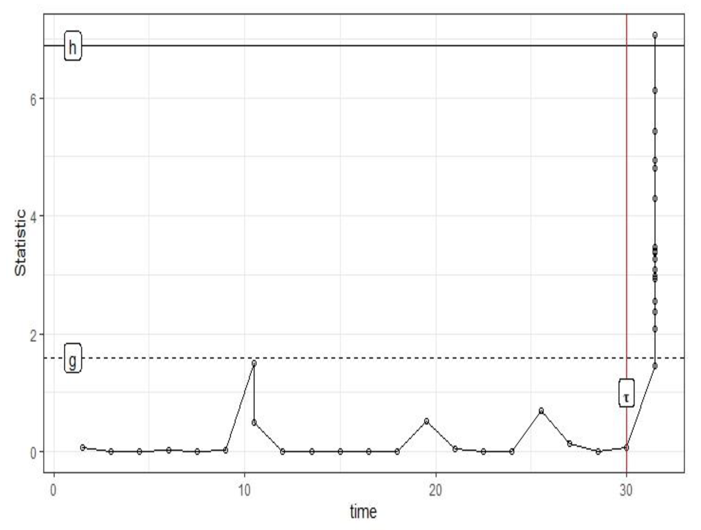
• If $R_{m,k,l}$ ≤ g, then at sampling point k, we will stop sampling and await till sampling point $k+1$ to be sampled accordingly. So, here the sample range at k sampling point is $n_k=l$ = l.
• In case $\mathrm{g}<R_{m,k,l}<h$ then we have two options which need to be followed.

  (i)

  Draw further analysis at point $k$.

  (ii)

  Move to stage (1) as addressed above, with the existing set of data points at the k sampling point specified as $l=l+1$.

• When $R_{m,k,l}>h$, subsequently indicates that there has been a shift in the parameter $\theta$.

The control chart limits g and h can be taken to convene the quantified in-control enactment necessities. We will examine the performance measure in the following segment.

3. Performance Measures

3.1. In-Control Performance Measurements

A specific signal emitted through a control chart stands a fictitious signal whenever the operation is in control. The fictitious signal activity can be calculated through the reciprocity of the time estimated towards an indication. Describe the average time to signal (ATS) as the intended span of phase since the beginning of the method observing to the spell of the map is signaling. Describes the average number of samples to signal (ANSS) to be the estimated number of samples since the beginning to the period of the project is sending indications. Evaluating two or more control charts obviously requires the same in-control ATS.

The number of data points acquired through every sampling fact is random whenever chronological testing is being used. Therefore, we intend to focus on the estimated number of observations to determine the average rate of sampling. Consider the average number of observations to signal (ANOS) to be the set of data points predicted after the commencement of method analysis towards the spell where the indication is produced. The average sampling rate per unit time can be represented by the ratio ANOS/ATS. The average in-control sampling rates and wrong signal rates would be the same for such charts, in case dissimilar control charts need the identical in-control ATS as well as the relatively similar ANOS.

The average sample number (ASN) is the estimated sample size in sequential analysis. By applying sequential analysis towards the procedure inspection, at each sample point we require the sample size to be estimated; thus, for each sampling stage, we require the ASN. After all, such ASN may not be consistent through various samples since both previous samples and the present sample rely on the sample size applied for a sampling point. So, the ASN description can be written as $ASN=ANOS/ANSS$, this is the cumulative sample size distributed over whole datasets prior to the warning.

3.2. Out-of-Control Performance Measurements

Once an alteration arises within the procedure, the ATS is sufficient to calculate the detection duration for such a change unless it appears at the beginning of the monitoring. In many situations, though, it would always be more reasonable to assume that the change happens after analysis begins at some uncertain time. The detection time should be determined for such functions as the estimated period from the random point when the change appears before an indication is produced. For such tasks, the steady-state ATS (SSATS) is sufficient. The predicted interval from the change to the sign indicates that perhaps the control parameter has approached its stable-state or static distribution by the specific time point that shift takes place. It, therefore, implies that the possibility of the change happening at a specific length in a sampling period is proportional to the product of the length of the duration and the static chance of using that interval where the static event is based on no wrong alerts arising until the change happens. In contrast, it ensures that the direction of the shift is evenly allocated around the span, whereas the change occurred in a sampling period.

The standardized shift δ used here to measure the size of the shift, where:

$$\delta =\frac{{\theta }_1}{{\theta }_0}.$$

The standards of δ are assumed that vary from 1.1 to 30. Several other categories were also examined, but as they lead to consistent assumptions therefore those findings are not displayed here.

3.3. The Extra Quadratic Loss

It typically occurs as some charts may perform superior at a specific period and some at any other shift size, particularly in comparing two control charts. Hence, the essential part is to provide any method which can be utilized to assess various control charts over a diverse variety of change scopes. For this reason, the quadratic loss in several articles has been utilized. For information and specific references to research on quadratic loss, see Yiming Peng and Marion R. Reynolds Jr (2014), [39], Reynolds and Lou (2010), [25].

It can be defined as a weighted average run length over the whole process domain of shifts (${\delta }_{min}<\delta <{\delta }_{max})$ employing a square of shift ${\delta }^2$ as weights. Arithmetically, this explanation follows:

$$EQL=\frac{1}{{\delta }_{max}-{\delta }_{min}}\underset{{\delta }_{min}}{\overset{{\delta }_{max}}{{\displaystyle \int }}}{\delta }^{2}ARL\left(\delta \right)d\delta ,$$

where A$RL\left(\delta \right)$ specifies the ARL value of a specific chart at the shift $\delta .$

4. Choosing the Parameters of the SS GLR Chart

We have to pick the value of window band m for the SS GLR chart, the $ASN$ that needs to be equal to the interval of sample $d$, as well as the limits $\mathrm{g}$ and $h$. Moreover, we will focus on providing optimum values of $ASN$ and $m$. For computing the $\mathrm{g}$ and $h$, the equations of regression will be developed considering the preferred in-control $ANOS$ and $ATS$.

4.1. The Window Size of the SS GLR Chart

The good aggregate output for a fixed sampling rate (FSR) GLR chart is achieved by taking window band $m$ to remain sufficiently big so as the GLR chart’s outcome with this window is the same as that of the GLR chart without window. For further information, please refer to Reynolds and Lou (2010), [25]. Conversely, we noticed that a much shorter window size would be better for the SS GLR chart.

Throughout this research, the efficiency of the control charts is investigated by simulation techniques with 10,000 iterations. To illustrate the influence of the window band upon the control chart’s sensitivity when monitoring process changes, SSATS values for various window sizes are computed. The control limits are chosen to achieve an in-control $ATS of 1400\left(AT{S}_0=1400\right)$, through which the shift is classified while $\delta =\theta /{\theta }_0$ besides $\theta >{\theta }_0$. All findings from the replication are recorded in

Table 1. SSATS and EQL values of SS GLR charts with ASN = d = 1.5 for different window sizes.

SS GLR Charts, ASN = 1.5, d = 1.5
m=	1	4	10	15	50	100	250
δ
1	1401.10	1401.10	1400.36	1400.22	1400.22	1400.05	1400.06
1.1	684.35	649.06	621.78	612.98	580.32	563.19	551.37
1.2	235.67	212.02	189.44	180.50	162.09	157.70	156.29
1.3	104.81	89.79	78.79	75.18	68.79	68.35	69.05
1.8	14.21	12.29	11.62	11.62	11.98	12.19	12.40
2	9.75	8.19	7.91	7.98	8.32	8.61	8.83
3	3.36	3.00	3.11	3.23	3.50	3.59	3.53
4	2.06	1.92	2.03	2.14	2.32	2.33	2.41
6	1.30	1.28	1.35	1.39	1.49	1.53	1.55
10	1.03	1.00	1.03	1.05	1.09	1.11	1.11
15	0.97	0.94	0.95	0.95	0.97	0.98	0.98
20	0.95	0.90	0.92	0.91	0.95	0.95	0.98
30	0.93	0.87	0.90	0.90	0.91	0.94	0.94
EQL=	106.48	99.45	97.90	97.06	95.99	96.07	96.08
h=	6.8373	6.8645	6.8773	6.8848	6.8853	6.8833	6.8763
g=	0.9290	1.1990	1.3633	1.4313	1.5945	1.6668	1.7428

Abbreviations: SSATS, steady-state average time to signal; EQL, extra quadratic loss; SS GLR, sequential sampling generalized likelihood ratio; ASN, average sample number.

and

Table 2. SSATS and EQL values of SS GLR charts with ASN = d = 5 for different window sizes.

SS GLR Charts, ASN = 5, d = 5
m=	1	5	10	20	50	100	150
δ
1	1401.33	1401.28	1401.23	1401.28	1401.10	1401.28	1401.55
1.1	361.71	351.00	345.32	343.02	343.42	343.10	343.92
1.2	128.78	108.02	104.86	103.55	105.14	105.21	103.47
1.3	74.96	51.56	51.73	54.12	56.24	54.43	53.77
1.8	13.91	13.83	13.38	15.47	15.21	14.70	14.57
2	15.31	9.53	10.25	12.01	12.63	12.82	12.55
3	6.85	4.64	4.42	4.24	4.17	4.29	4.16
4	3.33	3.27	3.13	3.41	3.41	3.49	3.31
6	2.72	2.28	2.23	2.25	2.38	2.29	2.38
10	2.59	2.06	1.98	2.03	2.11	2.04	2.11
15	2.49	1.98	1.93	1.95	2.03	2.03	2.03
20	2.45	1.97	1.88	1.91	2.00	2.00	2.00
30	2.40	1.86	1.81	1.89	1.92	1.99	1.99
EQL=	173.83	139.48	135.76	139.33	142.96	144.48	144.54
h=	5.6545	5.6016	5.5997	5.5937	5.5902	5.5897	5.5890
g=	0.3373	0.4309	0.4545	0.4804	0.5069	0.5151	0.5238

Abbreviations: SSATS, steady-state average time to signal; EQL, extra quadratic loss; SS GLR, sequential sampling generalized likelihood ratio; ASN, average sample number.

.

We observed that the outputs are better through Table 1, and the optimum window is smaller than the FSR GLR charts, which is reported to be m = 50 for ASN = 1.5. We took ASN = d = 1.5 and ASN = d = 5, with ${\theta }_0=0.001$, for the simulation analysis and the first type geometric data (a = 0) is considered for simulation results. Considering the situation wherein 1.5 is assigned to be the in-control ASN. In Table 1 and Table 2, the values of $EQL$ and $SSATS$ are given for different shifts.

We can see in Table 1 that the EQL as a mechanism of m is relatively flat across the minimal, that seems to stand about 50. Notice that the rate of g correspondingly rises as m increases, however, h appears relatively stable for, $m>1$. Usually, wide window sizes may assist rapidly identify minor changes, however, harm the recognition performance for middle to broad change types. In this case, the window size 50 ensures a proper fit for ASN 1.5, which brings an EQL value comparable to the optimum.

Table 2 indicated that the optimal window band to monitor a wide range of shifts upon this SS GLR control chart is m = 10. For geometric observations with a big ASN, such as ASN = 5 for the SS GLR control chart is useful for recognizing large parameter changes. We can see from Table 1 and Table 2, that for geometric observation, the bigger ASN makes the performance more feasible and the optimum window size became lower as m = 10 with ASN = 5.

The explanation of how a lesser window band provides finest results for the SS GLR chart is one logical point that can be raised here, whereas a big window size is superlative for the FSR GLR chart. Let us focus on a schematic of the SS GLR chart to help address this query.

The pattern of the SS geometric GLR chart statistics, relying on a single replication, is shown in Figure 1. We assign the in-control ASN of 1.5, at every 1.5-time unit, the samples have been drawn. Through time point 30, the mechanism was in control, and then a shift to δ = 2 was implemented. Here, the optimum window size chosen that is, $m=50$. From the figure, $h$ is shown through the solid horizontal line, while $\mathrm{g}$ is shown by the horizontal dashed line that is determined to provide 144.22 in-control $ANOS$ and $ATS$ values.

Points interconnected with a vertical line in Figure 1 suggest that these came from the identical sample. For instance, at time 1.5, the primary sample was collected, a consumed single observation; at point 3 and 4.5, the second and third sample was collected, likewise a consumed single observation, at point 6, the fourth sample was collected and had two observations, and so on. Much of the samples were of size $n_i=1$ once the procedure remained in control (by time 30), with some of those with $n_i>1$. Fortunately, $R_{m,k,l}$ rapidly moved beyond g after the process went out of control (afterwards time 30), and the sampling rate dramatically boosted, as can be seen in the plot. As soon as there was some hint in the mechanism that a shift at the existing sampling point may have emerged, further samples were taken unless either a signal was obtained or there was proof that there has been no process shift and at the next sampling point, a new sample was taken. Which is why, though with limited window size, further observations can be examined as required once there is some sign of a process shift. In the FSR GLR chart, the justification for choosing a big window size is that many observations are required to identify tiny changes. The data from a big number of observations will still be included in the SS GLR chart, even if the window size is limited, as displayed in Figure 1.

4.2. The Control Limits of SS GLR Chart

The SS GLR chart generally has to control limits $\mathrm{g}$ and $h$ which are required to be identified. These two constraints define the in-control $ASN$ and $ANOS$. For the specific estimation of $\mathrm{g}$ and $h$ for defined outcomes of the in-control $ASN$ and $ANOS$, the regression equations for a geometrically distributed process with the optimum window size 50 are given. In which a represents ASN in these formulations and l describes log₁₀ ANOS:

$$\begin{array}{cc}g=9.42395673l& -10.89098644al-2.29613669l^2+4.46278765a^{2}l\\ & +2.67440159a{l}^2-1.13860016a^2{l}^2-0.73038401a^3\\ & +0.04130327l^3+0.01294851a^3{l}^3,\end{array}$$

$$\begin{array}{cc}h=1.95856229199l& -0.91034870256al+0.49652649209l^2+0.19816069956a^{2}l\\ & +0.14521861865a{l}^2-0.03129397100a^2{l}^2-0.03230190673a^3\\ & -0.08470173390l^3+0.00006706498a^3{l}^3.\end{array}$$

The calculations as mentioned above can generate the approximate parameters for the SS GLR chart when an expert takes certain ideal standards for the in-control $ASN$ and $ANOS$. To the required in-control $ATS$ or the necessary rate of sampling, the sampling interim d may be specified. The ratio of in-control $ATS/d$ can be used to determine the in-control $ANOS$.

The $\mathrm{g}$ and $h$ equations were attained through the regression equations using 1000 simulations, $ASN$ standards, and ATS values for the limit g ranging from 0.8 to 2, and h is from 6 to 10. The resulting ASN and ATS range from 1.2 to 3.67 and 527.11 to 53366.36, respectively. For both equations, the coefficients of determination are more significant than 0.999. The particular values of $\mathrm{g}$ and $h$ can be obtained by using the equation given above.

5. Performance Comparisons with Other Charts

We are instantly analyzing the SS geometric GLR chart’s output compared to other control charts. Initially, we contemplate the GLR chart for detecting the parameter changes in a geometrically distributed mechanism examined by KazemiNia A, Gildeh BS, Abbasi Ganji Z (2018), [40]. From this analysis, we will see the enhancement in the GLR chart efficiency arising from the use of a sequential sampling scheme.

5.1. Comparison with the Geometric GLR Chart

The geometric GLR chart uses a static sample amount of $n$ and a fixed sampling interval of $d$ to take measurement. Therefore, we considered the geometric GLR chart by $n=d$ for comparing the results with the SS geometric GLR chart, here $n=d=5$ and the in-control sampling rate one is considered.

It is suggested that the geometric GLR chart’s window size be large sufficient so that its output appears identical to the FSR GLR chart exclusive of the window. The window size is assumed to be m = 100, 160, 180, 200, and 300, for the geometric chart, while for SS geometric, we deliberate the lesser window band. The geometric GLR chart statistic $R_{m,k,l}$ is identical to the SS geometric GLR chart excluding that it is computed following the whole illustration of n observations are achieved at sampling point k (check Reynolds and Lou, 2010 for further information).

Table 3. SSATS and EQL values of SS GLR charts with ASN = n = 5 for different window sizes.

SS Geometric GLR Chart					Geometric GLR Chart
ASN = n = 5
m=	1	5	10	50	100	100	160	180	200	300
δ
1	1401.33	1401.28	1401.23	1401.1	1401.28	1400.6	1400.45	1400.05	1400.9	1400.9
1.1	361.71	351	345.32	343.42	343.1	421.35	353.6	356.3	355.7	354.05
1.2	128.78	108.02	104.86	105.14	105.21	174.95	175.35	175.45	175.6	175.75
1.3	74.96	51.56	51.73	56.24	54.43	129.1	127.3	128.5	128.9	129
1.8	13.91	13.83	13.38	15.21	14.7	30.95	31.05	31.55	31.7	31.8
2	15.31	9.53	10.25	12.63	12.82	24.25	24.35	24.55	24.55	24.65
3	6.85	4.64	4.42	4.17	4.29	10.85	10.9	10.8	10.85	10.9
4	3.33	3.27	3.13	3.41	3.49	7.95	7.95	7.95	8	8.05
6	2.72	2.28	2.23	2.38	2.29	5.55	5.65	5.65	5.65	5.7
10	2.59	2.06	1.98	2.11	2.04	3.55	3.55	3.55	3.6	3.6
15	2.49	1.98	1.93	2.03	2.03	2.55	2.55	2.55	2.55	2.55
20	2.45	1.97	1.88	2	2	2.55	2.55	2.55	2.55	2.55
30	2.4	1.86	1.81	1.92	1.99	2.5	2.5	2.5	2.5	2.5
EQL=	173.83	139.48	135.76	142.96	144.48	248.31	245.56	245.79	246.05	246.13
h=	5.6545	5.6016	5.5997	5.5902	5.5897	5.576	5.592	5.608	5.624	5.64
g=	0.3373	0.4309	0.4545	0.5069	0.5151	-	-	-	-	-

Abbreviations: SSATS, steady-state average time to signal; EQL, extra quadratic loss; SS GLR, sequential sampling generalized likelihood ratio; ASN, average sample number.

provides $EQL$ and $SSATS$ values for the SS geometric GLR chart and the non-sequential geometric GLR chart. The initial four columns display the SS geometric GLR chart outcomes, besides the subsequent four columns illustrate the findings for the non-sequential geometric GLR chart. $ASN=n=5$ is used on behalf of the SS geometric GLR chart. Note that the limit g is not required in the FSR geometric GLR chart. As a whole, while d is identical by way of both charts, the output of the SS geometric GLR chart is significantly higher compared to the non-sequential geometric GLR chart, as in Table 3. The SSATS results of the SS geometric GLR chart are considerably lower than the non-sequential geometric GLR charts for minor shifts. Their output is relatively close for large shifts, but SS geometric has still been performing better. Moreover, the optimum window of SS geometric for $ASN=5$ is 10, which devises superior functioning compared to the optimum window size of the geometric GLR chart, which is 160 for $n=5$.

5.2. Comparison with the CUSUM Geometric Chart

The cumulative sum chart integrates previous data into every illustrated inspection. The CUSUM chart consumes better efficiency. The CUSUM chart, besides, is little susceptible to the presumption of normality. The CUSUM chart indication rate regulates the compassion to identify extremely tiny changes; see Brook and Evans, Reynolds, and Stoumbos and Szarka and Woodall, [41,42,43].

Based on

Table 4. SSATS and EQL values of SS GLR charts with ASN = d = 5 for different window sizes.

SS Geometric GLR Chart					CUSUM Geometric Chart
ASN = n = 5
m=	1	5	10	50	100	δ1 = 1.1	1.5	1.7	1.8	2
δ
1	1401.33	1401.28	1401.23	1401.1	1401.28	1400.4	1400.45	1400.1	1400.7	1400.1
1.2	128.78	108.02	104.86	105.14	105.21	148.6	135.15	167	198.65	227.25
1.3	74.96	51.56	51.73	56.24	54.43	89.2	92	113.6	121.4	146.95
1.8	13.91	13.83	13.38	15.21	14.7	37.2	27.2	25.6	25.85	27.3
2	15.31	9.53	10.25	12.63	12.82	31.35	22.05	20.3	19.7	20.4
3	6.85	4.64	4.42	4.17	4.29	22.3	13.55	12.1	11.35	10.5
4	3.33	3.27	3.13	3.41	3.49	18.95	11.7	10.15	9.55	8.8
6	2.72	2.28	2.23	2.38	2.29	17.6	10.05	7.8	7.2	6.8
10	2.59	2.06	1.98	2.11	2.04	15.4	9.85	6.9	6.9	6.75
15	2.49	1.98	1.93	2.03	2.03	16.45	9.8	7.1	7.05	7.05
20	2.45	1.97	1.88	2	2	15.2	8.95	7	7.05	6.85
30	2.4	1.86	1.81	1.92	1.99	14.65	7.2	6.75	6.8	6.7
h=	5.6545	5.6016	5.5997	5.5902	5.5897	2.112	3.864	4	4.096	4.264
g=	0.3373	0.4309	0.4545	0.5069	0.5151	-	-	-	-	-

Abbreviations: SSATS, steady-state average time to signal; SS GLR, sequential sampling generalized likelihood ratio; CUSUM, cumulative sum chart; ASN, average sample number.

, the CUSUM plan has superior functioning than the GLR geometric charts besides SS geometric GLR charts in discovering certain minor constraint changes for ${\delta }_1=1.1$. Still, the CUSUM chart cannot blow the other two charts in finding big constraint changes. The CUSUM chart through ${\delta }_1=1.7$ appears to be superior to the geometric GLR chart in observing two intermediary shifts $\delta =1.8$ and $\delta =2$, but cannot beat the SS geometric GLR chart performance.

Overall, the performance of the SS geometric GLR control chart consistently accomplishes superior to the geometric GLR and CUSUM control charts for almost all setup parameter shift cases. We advise utilizing the sequential sampling GLR chart when monitoring the parameter shifts for the geometrically distributed process.

6. Conclusions

The purpose of monitoring is considered in this article to identify a broad choice of shifts quickly in a geometrically distributed procedure. The SS GLR control chart’s outputs are also compared to two standard counterparts, the non-sequential GLR and the CUSUM chart. We have presented that the SS GLR chart performs significantly superior compared to other control charts.

In specific process control purposes, the process measurements become possible sequentially due to the design of the analysis or evaluation method. In these instances, the practice of sequential sampling appears to be normal. While implementing the sequential sampling scheme, the potential to track process modifications or declined sampling rates can be drastically enhanced. Whenever the sequential sampling plan is viable in implementations, we suggest using the SS GLR.

The SS GLR charts take the benefit that several chart factors do not require to be defined by practitioners. Practitioners are required to determine the sampling rate d, the in-control $ASN$, and the in-control $ATS$ value to model the SS GLR chart for their purpose and implement the given regression equations to extract the $\mathrm{g}$ and $h$ limits.

In the GLR control chart, the control limit and window size calculation depend on simulations. To evaluate the control limit, further simulations need to be carried out.

References

- Xie, M.; Goh, T.N.; Kuralmani, V. Statistical Models and Control Charts for High-Quality Processes; Springer Science and Business Media: Berlin/Heidelberg, Germany, 2012. [Google Scholar]
- Shewhart, W.A. Economic Control of Quality of Manufactured Product; Macmillan And Co Ltd.: London, UK, 1931. [Google Scholar]
- Westgard, J.O.; Groth, T.; Aronsson, T.; De Verdier, C.H. Combined Shewhart-cusum control chart for improved quality control in clinical chemistry. Clin. Chem. 1977, 23, 1881–1887. [Google Scholar] [CrossRef] [PubMed]
- Wu, Z.; Yang, M.; Jiang, W.; Khoo, M.B. Optimization designs of the combined Shewhart-CUSUM control charts. Comput. Stat. Data Anal. 2008, 53, 496–506. [Google Scholar] [CrossRef]
- Lorden, G. Procedures for reacting to a change in distribution. Ann. Math. Stat. 1971, 42, 1897–1908. [Google Scholar] [CrossRef]
- Sparks, R.S. CUSUM charts for signalling varying location shifts. J. Qual. Technol. 2000, 32, 157–171. [Google Scholar] [CrossRef]
- Zhao, Y.; Tsung, F.; Wang, Z. Dual CUSUM control schemes for detecting a range of mean shifts. IIE Trans. 2005, 37, 1047–1057. [Google Scholar] [CrossRef]
- Han, D.; Tsung, F.; Hu, X.; Wang, K. CUSUM and EWMA multi-charts for detecting a range of mean shifts. Stat. Sin. 2007, 17, 1139–1164. [Google Scholar]
- Jackson, J.E. All count distributions are not alike. J. Qual. Technol. 1972, 4, 86–92. [Google Scholar] [CrossRef]
- Sheaffer, R.L.; Leavenworth, R.S. The negative binomial model for counts in units of varying size. J. Qual. Technol. 1976, 8, 158–163. [Google Scholar] [CrossRef]
- Bourke, P.D. Detecting a shift in fraction nonconforming using run-length control charts with 100% inspection. J. Qual. Technol. 1991, 23, 225–238. [Google Scholar] [CrossRef]
- Feller, W. An Introduction to Probability Theory and Its Application Vol II; John Wiley and Sons: Hoboken, NJ, USA, 1971. [Google Scholar]
- Benneyan, J.C. Performance of number-between g-type statistical control charts for monitoring adverse events. Health Care Manag. Sci. 2001, 4, 319–336. [Google Scholar] [CrossRef]
- Santiago, E.; Smith, J. Control charts based on the exponential distribution: Adapting runs rules for the t chart. Qual. Eng. 2013, 25, 85–96. [Google Scholar] [CrossRef]
- Montgomery, D.C. Control charts for variables. Introduction to Statistical Quality Control, Arizona, 6rd ed.; Wiley: Hoboken, NJ, USA, 2009; pp. 226–268. [Google Scholar]
- Kim, B.J.; Lee, J. Adjustment of control limits for geometric charts. Commun. Stat. Appl. Methods 2015, 22, 519–530. [Google Scholar] [CrossRef]
- Chang, T.C.; Gan, F.F. Cumulative sum charts for high yield processes. Stat. Sin. 2001, 11, 791–805. [Google Scholar]
- Xie, W.; Xie, M.; Goh, T.N. A Shewhart-like charting technique for high yield processes. Qual. Reliab. Eng. Int. 1995, 11, 189–196. [Google Scholar] [CrossRef]
- Quesenberry, C.P. Geometric Q charts for high quality processes. J. Qual. Technol. 1995, 27, 304–315. [Google Scholar] [CrossRef]
- Kaminsky, F.C.; Benneyan, J.C.; Davis, R.D.; Burke, R.J. Statistical control charts based on a geometric distribution. J. Qual. Technol. 1992, 24, 63–69. [Google Scholar] [CrossRef]
- Willsky, A.; Jones, H. A generalized likelihood ratio approach to the detection and estimation of jumps in linear systems. IEEE Trans. Autom. Control 1976, 21, 108–112. [Google Scholar] [CrossRef] [Green Version]
- Siegmund, D.; Venkatraman, E.S. Using the generalized likelihood ratio statistic for sequential detection of a change-point. Ann. Stat. 1995, 23, 255–271. [Google Scholar] [CrossRef]
- Hawkins, D.M.; Zamba, K.D. Statistical process control for shifts in mean or variance using a changepoint formulation. Technometrics 2005, 47, 164–173. [Google Scholar] [CrossRef]
- Lai, T.L.; Shan, J.Z. Efficient recursive algorithms for detection of abrupt changes in signals and control systems. IEEE Trans. Autom. Control 1999, 44, 952–966. [Google Scholar]
- Reynolds, M.R., Jr.; Lou, J. An evaluation of GLR control chart combined with an X chart. J. Qual. Technol. 2010, 42, 287–310. [Google Scholar] [CrossRef]
- Huang, W.; Reynolds, M.R., Jr.; Wang, S. A binomial GLR control chart for monitoring a proportion. J. Qual. Technol. 2012, 44, 192–208. [Google Scholar] [CrossRef]
- Huang, W.; Wang, S.; Reynolds, M.R., Jr. A generalized likelihood ratio chart for monitoring Bernoulli processes. Qual. Reliab. Eng. Int. 2013, 29, 665–679. [Google Scholar] [CrossRef]
- Lee, J.; Peng, Y.; Wang, N.; Reynolds, M.R., Jr. A GLR control chart for monitoring a multinomial process. Qual. Reliab. Eng. Int. 2017, 33, 1773–1782. [Google Scholar] [CrossRef]
- Arnold, J.C.; Reynolds, M.R., Jr. CUSUM control charts with variable sample sizes and sampling intervals. J. Qual. Technol. 2001, 33, 66–81. [Google Scholar] [CrossRef]
- Park, C.; Reynolds, M.R., Jr. Economic design of a variable sampling rate X chart. J. Qual. Technol. 1999, 31, 427–443. [Google Scholar] [CrossRef]
- Prabhu, S.S.; Runger, G.C.; Keats, J.B. X chart with adaptive sample sizes. Int. J. Prod. Res. 1993, 31, 2895–2909. [Google Scholar] [CrossRef]
- Reynolds, M.R., Jr. Shewhart and EWMA variable sampling interval control charts with sampling at fixed times. J. Qual. Technol. 1996, 28, 199–212. [Google Scholar] [CrossRef]
- Reynolds, M.R., Jr. Variable-sampling-interval control charts with sampling at fixed times. IIE Trans. 1996, 28, 497–510. [Google Scholar] [CrossRef]
- Reynolds, M.R.; Amin, R.W.; Arnold, J.C.; Nachlas, J.A. Charts with variable sampling intervals. Technometrics 1988, 30, 181–192. [Google Scholar] [CrossRef]
- Reynolds, M.R.; Stoumbos, Z.G. The SPRT chart for monitoring a proportion. IIE Trans. 1998, 30, 545–561. [Google Scholar] [CrossRef]
- Stoumbos, Z.G.; Reynolds, M.R., Jr. Control charts applying a general sequential test at each sampling point. Seq. Anal. 1996, 15, 159–183. [Google Scholar] [CrossRef]
- Stoumbos, Z.G.; Reynolds, M.R., Jr. Control charts applying a sequential test at fixed sampling intervals. J. Qual. Technol. 1997, 29, 21–40. [Google Scholar] [CrossRef]
- Stoumbos, Z.G.; Reynolds, M.R., Jr. The SPRT control chart for the process mean with samples starting at fixed times. Nonlinear Anal. Real World Appl. 2001, 2, 1–34. [Google Scholar] [CrossRef]
- Peng, Y.; Reynolds, M.R., Jr. A GLR Control Chart for Monitoring the Process Mean with Sequential Sampling. Seq. Anal. Des. Methods Appl. 2014, 33, 298–317. [Google Scholar] [CrossRef]
- KazemiNia, A.; Gildeh, B.S.; Abbasi Ganji, Z. The design of geometric generalized likelihood ratio control chart. Qual. Reliab. Eng. Int. 2018, 34, 953–965. [Google Scholar]
- Brook, D.A.E.D.; Evans, D. An approach to the probability distribution of CUSUM run length. Biometrika 1972, 59, 539–549. [Google Scholar] [CrossRef]
- Reynolds, M.R., Jr.; Stoumbos, Z.G. A CUSUM chart for monitoring a proportion when inspecting continuously. J. Qual. Technol. 1999, 31, 87–108. [Google Scholar] [CrossRef]
- Szarka III, J.L.; Woodall, W.H. On the equivalence of the Bernoulli and geometric CUSUM charts. J. Qual. Technol. 2012, 44, 54–62. [Google Scholar] [CrossRef]