Point Cloud Coding Solutions, Subjective Assessment and Objective Measures: A Case Study

Abstract

This paper presents a summary of recent progress in compression, subjective assessment and objective quality measures of point cloud representations of three dimensional visual information. Different existing point cloud datasets, as well as discusses the protocols that have been proposed to evaluate the subjective quality of point cloud data. Several geometry and attribute point cloud data objective quality measures are also presented and described. A case study on the evaluation of subjective quality of point clouds in two laboratories is presented. Six original point clouds degraded with G-PCC and V-PCC point cloud compression and five degradation levels were subjectively evaluated, showing high inter-laboratory correlation. Furthermore, performance of several geometry-based objective quality measures applied to the same data are described, concluding that the highest correlation with subjective scores is obtained using point-to-plane measures. Finally, several current challenges and future research directions on point clouds compression and quality evaluation are discussed.

1. Introduction

A point cloud is a set of discrete data points defined in a given coordinate space—for example 3D Cartesian coordinate system, representing samples of surfaces of objects, urban landscapes or other three-dimensional physical entities. To create point clouds, active or passive methods can be used. Examples of active methods include processes based on structured light, scanning laser ranging and full-front laser or radio-frequency sensing, while passive methods include capturing multi-view images and videos followed by a triangulation procedure to generate the cloud of points representing the scene or object(s). 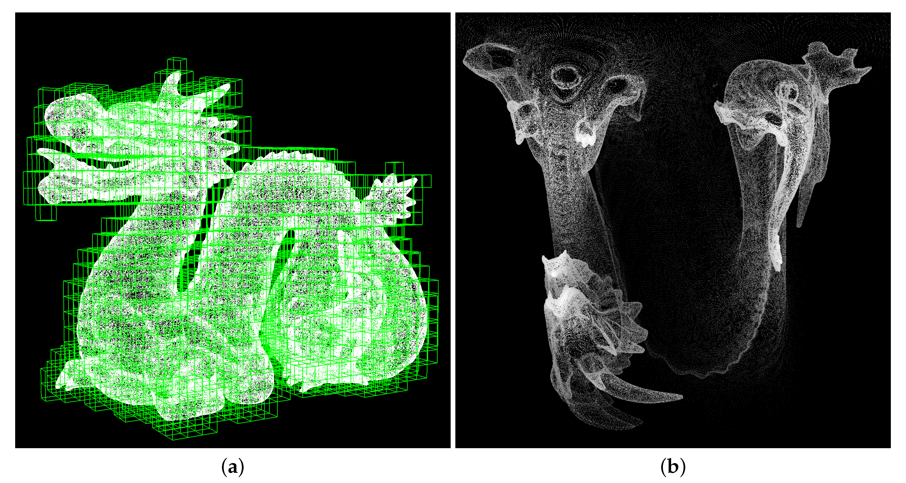Point cloud displaying can be done directly, showing the raw points on 2D or 3D displays or by displaying approximating surfaces after applying a suitable reconstruction algorithm [1]. An example point cloud, “dragon”, from [2], is shown in Figure 1, where the left image shows the point cloud points rendered directly and viewed from a specific observation point and the right image shows the same point cloud after surface reconstruction using volumetric merging [3] (viewed from the same point).

Point clouds can have from a few hundred thousand to several million points and require tens of megabytes for storing the set of point coordinates and (optional) point attributes such as color and normal vector information. Efficient storage and transmission of such massive data volumes thus requires the use of compression techniques. Several recent point cloud compression methods are briefly described next, covering geometry-based compression algorithms (e.g., Geometry-based Point Cloud Compression, G-PCC) and projection-based compression algorithms (e.g., Video-based Point Cloud Compression, V-PCC). New neural network based compression methods are also presented.

Recently, the JPEG standardization committee (ISO/IEC JTC 1/SC 29/WG 1) created a project called JPEG Pleno aimed at fostering the development and standardization of a framework for coding new image modalities such as light field images, holographic volumes, and point cloud 3D representations [4]. As part of this effort, a JPEG Ad Hoc Group on Point Clouds compression (JPEG PC AhG) was created within JPEG Pleno, with mandates to first define different subjective quality assessment protocols and objective measures for use with point clouds and later lead activities geared towards standardization of static point cloud compression technologies.

This paper presents an overview of existing methods for point cloud compression and the research problems involved in evaluating the perceived (subjective) visual quality of point clouds and estimating that quality using computable models, using some of the activities of the JPEG PC AhG as a case study. The paper is focused on these specific activities first and foremost because they are the first large-scale series of studies aiming at evaluating the subjective and objective quality of point clouds in a systematic and organized way and secondly because of the direct involvement of the authors in conducting a significant part of that work.

The structure of this article is as follows. Section 2 presents recent coding solutions that have been proposed for compressing point cloud data. Section 3 describes the materials and methods involved in subjective evaluation of point clouds quality. A list of some recent point cloud test datasets is presented, and then the protocols that have been proposed to evaluate the subjective quality of point clouds are described. Section 4 presents point cloud objective quality measures/estimators for the geometry and attribute components, some operating on the 3D point cloud information and others based on the projection of the points onto 2D surfaces. Section 5 present protocols to process and analyze subjective mean opinion scores (MOS) and different correlation measures used to compute the agreement between subjective quality scores and objective quality measures/estimates. Section 6 describes one case study involving a subjective evaluation of compressed point clouds and respective objective quality computations. Finally, Section 7 closes the article with some conclusions.

2. Point Cloud Coding Solutions

In [5], an efficient octree-based method used to store and compress 3D data without loss of precision is proposed. The authors demonstrated its usage in an open file format for interchange of point cloud information, fast point cloud visualization and to speed-up 3D scan matching and shape detection algorithms. This octree-based compression algorithm (with arbitrarily chosen octree depth), is a part of the “3DTK—The 3D Toolkit” [6]. As described in [7], octree-based representations can be used with nearest neighbor search (NNS) algorithms, in applications such as shape registration and, as explained below, in geometry-based point cloud objective quality measures.

MPEG’s G-PCC (Geometry based Point Cloud Compression) codec [8] is a geometry octree-based point cloud compression codec which can use trisoup surface approximations. It merges the L-PCC (LIDAR point cloud compression for dynamic point clouds) coder and the S-PCC (Surface point cloud compression for for static point clouds) coder, previously defined by the MPEG standards committee, into a coding method that is appropriate for sparse point clouds. Currently, G-PCC only supports intra prediction, that is, it does not use any temporal prediction tool. G-PCC encodes the content directly in 3D space in order to create the compressed point cloud. In lossless intra-frame mode, the G-PCC codec currently provides an estimated compression ratio up to 10:1, while lossy coding with acceptable quality can be done with compression ratios up to 35:1. In G-PCC, geometry and attribute information are encoded separately. However, attribute coding depends on geometry, thus geometry coding is performed first. Geometry encoding starts with a coordinate transformation followed by a voxelization, after which a geometry analysis is done either using an octree decomposition or a trisoup (“triangle soup”) surface approximation scheme. Finally, arithmetic coding is applied to achieve lower bitrates. Regarding the attribute coding, three options are available: Region Adaptive Hierarchical Transform (RAHT), Predicting Transform, and a Lifting Transform. After application of one of these transforms, the coefficients are quantized and arithmetically encoded.

MPEG’s V-PCC (Video based Point Cloud Compression) codec [9] projects the 3D points onto a set of 2D patches that are encoded using legacy video technologies, such as H.265/HEVC video compression [10]. The current V-PCC encoder compresses dynamic point cloud with acceptable quality with a compression ratio up to 125:1; thus, for example, a dynamic point cloud with one million points could be encoded at 8 Mbit/s. V-PCC firstly generates 3D surface segments by dividing the point cloud into a number of connected regions, using information from normal vectors from each point. Those 3D surface segments are called patches and each 3D patch is afterwards independently projected into a 2D patch. This approach helps to reduce projection issues, such as occlusions and hidden surfaces. Each 2D patch is represented by a binary image, the occupancy map, which signals if a pixel is present in 3D projected point, a geometry image that contains the depth information (depth map) and a set of images that represent the projected points attributes (e.g., R, G, B channels for full-color point clouds or a luminance channel for grayscale point clouds). The 2D patches are packed/padded in a 2D image/plane with several optimizations to use the minimum possible space 2D space. This procedure is applied to the occupancy map, the geometry map, and the texture map. Additionally, different algorithms are used to smooth transitions between patches in the same image, and to adjust subsequent patches in time for better compression efficiency. After the sequences of 2D images containing the packed patches are created, they are compressed using H.265/HEVC video compression, although any other compression might be used as well. The geometry images are represented in the YUV420 color space, with information in the luminance channel only. The texture images are represented in RGB444 and then converted to YUV420 before coding. The occupancy map is a binary image that is coded using specifically developed lossless video encoder [11], but lossy encoding can also be used [12]. Recently, the V-PCC codec for dynamic point clouds has been tested [13] with very good results. For more details about G-PCC and V-PCC, please check [14,15].

Other point cloud coding solutions have also been proposed in recent years. He et al. [16] proposed a best-effort projection scheme, which uses joint 2D coding methods to effectively compress the attributes of the original 3D point cloud. The scheme includes lossless and lossy modes, which can be selected according to different requirements. In [17], the authors presented a point cloud compression algorithm based on projections. Different projection types have been tested, using the framework from “3DTK—The 3D Toolkit” [6], namely equirectangular, Mercator, cylindrical, Pannini, rectilinear, stereographic, and Albers equal-area conic projections. Different compression ratios are achieved by using different resolution for projection images. In [18], the same authors proposed compressing 3D point clouds using panorama images generated with equirectangular projection, to encode the range, reflectance, and color information of each point. Lossless and JPEG lossy compression methods have been tested to encode the projections.

Novel neural network based point cloud compression methods have also been proposed recently. In [19], the authors proposed a new method for static point cloud data-driven geometric compression based on learned convolutional transform and uniform quantization. In terms of rate-distortion, the proposed method is superior to the MPEG reference software. Wang et al. [20] proposed deep neural network-based variational autoencoders to efficiently compress point cloud geometry information. the reported results show higher compression efficiency than that of MPEG’s G-PCC.

Figure 2 shows two examples of representations using 3D structures and 2D images. The left image shows an octree decomposition (with five levels) of the “dragon” point cloud, obtained using CloudCompare [21], and on the right an equirectangular 2D projection of the same point cloud computed using 3DTK toolkit [6] is presented.

3. Subjective Assessment of Point Cloud Quality

Quality of experience is defined, according to the COST Action Qualinet, as “The degree of delight or annoyance of the user of an application or service” [22]. QoE is influenced by several factors that can be generally divided into three main categories: human-related, system-related, and context-related factors. To measure QoE of different multimedia signals, subjective assessment of the quality can be performed, representing quality of each tested content item by a single number (which, in some cases, may be not enough to fully describe QoE [23]). For example, in a typical subjective image or video quality assessment campaign, observers watch a series of original and degraded images or video sequences and rate their quality numerically. The subjective quality of a specific image or video is measured by the average of all users ratings for that image or video, i.e., using a Mean Opinion Score (MOS), which is regarded as the quality score that the average viewer would assign to that particular image or video. MOS scores are collected according to the well-defined methods and procedures proposed in recent decades and aimed at guaranteeing the use of the same experimental settings and conditions during different assessments.

Commonly used subjective image and video quality assessment methods are proposed in recommendation ITU-R BT.500-14 [24]. This recommendation (and others related) defines single or double stimulus methods to perform subjective quality assessment, depending on how the content is shown to the observer. Some of the methods defined are “Single-Stimulus” (SS), “Double Stimulus Continuous Quality Scale” (DSCQS), “Stimulus-Comparison” (SC), and “Single Stimulus Continuous Quality Evaluation“ (SSCQE). The most common subjective quality assessment method is the DSCQS procedure, in which the observer grades a pair of images or video sequences coming from the same source, one of which, the original or reference signal, is observed directly without any further processing and the other goes through a test system which is either real or simulates a real system, resulting in the processed or test signal. The observer grades both the original and processed signals, usually on a differences scale, resulting in a group of scores that represent the perceptual difference between the reference and test videos (or images). Alternative methods for estimating image or video sequences have been proposed, such as the one-step continuous quality evaluation (SSCQE) procedure, in which users evaluate images or video sequences that contain impairments that differ over time, such as those obtained by different encoding parameters.

Currently, subjective evaluation of point clouds is not standardized yet; however, similar procedures can be adapted as in the usual image/video quality assessment methods that are defined in in ITU-R BT.500-14 [24]. Possible subjective evaluations of point clouds include interactive or passive presentation, different viewing technologies (e.g., 2D, 3D, immersive video, and image displays), and raw point clouds or point clouds after surface reconstruction. Surface reconstruction may be used because observers can easier observe and afterwards grade them. However, for more complex point clouds, as well as noisy point clouds, surface reconstruction may produce unwanted artifacts not directly related to compression or take too long to compute. If subjective experiments are being made using raw point clouds, point size is usually adjusted by expert viewing to obtain watertight surfaces. Virtual camera distance and camera parameters may also be adjusted according to the expected screen resolution.

The next subsections describe different protocols that have been proposed to evaluate the subjective quality of different point cloud datasets. Section 3.1 identifies and describes the point cloud datasets publicly available that have been used in recent works, and Section 3.2 reviews recent subjective point cloud quality evaluation studies summarizing the procedures followed in preparing the point clouds for presentation to the graders/observers, the choice of rendering method (raw point vs. rendered surface), the presentation protocols adopted (interactive or passive), and the viewing technologies employed.

3.1. Point Cloud Datasets

Many different point cloud datasets have been proposed recently, for studies related to different application tasks such as shape classification, object classification, semantic segmentation, shape generation, and representation learning. Point cloud datasets used to train and test deep learning algorithms for different applications are described in detail in [25,26]. Here, we briefly mention some of the point cloud datasets that have been used in applications where the end user is a human being, namely those proposed in the context of JPEG standard creation activities. One of the first tasks undertaken by the participants of the JPEG Pleno project was the collection and organization of raw point cloud datasets to be used in the activities planned to follow. Several static point clouds with different sources were collected and made publicly available at the JPEG Pleno test content archive [27]. The dataset includes point clouds originally sourced from “8i Voxelized Full Bodies (8iVFB v2)” [28], “Microsoft Voxelized Upper Bodies”, “ScanLAB Projects: Science Museum Shipping Galleries point cloud data set”, “ScanLAB Projects: Bi-plane point cloud data set”, “UPM Point-cloud data”, and “Univ. Sao Paulo Point Cloud dataset.” For details, see information provided in [27]. Another repository for 3D point clouds from robotic experiments can be found in [29], a part of the 3DTK toolkit datasets.

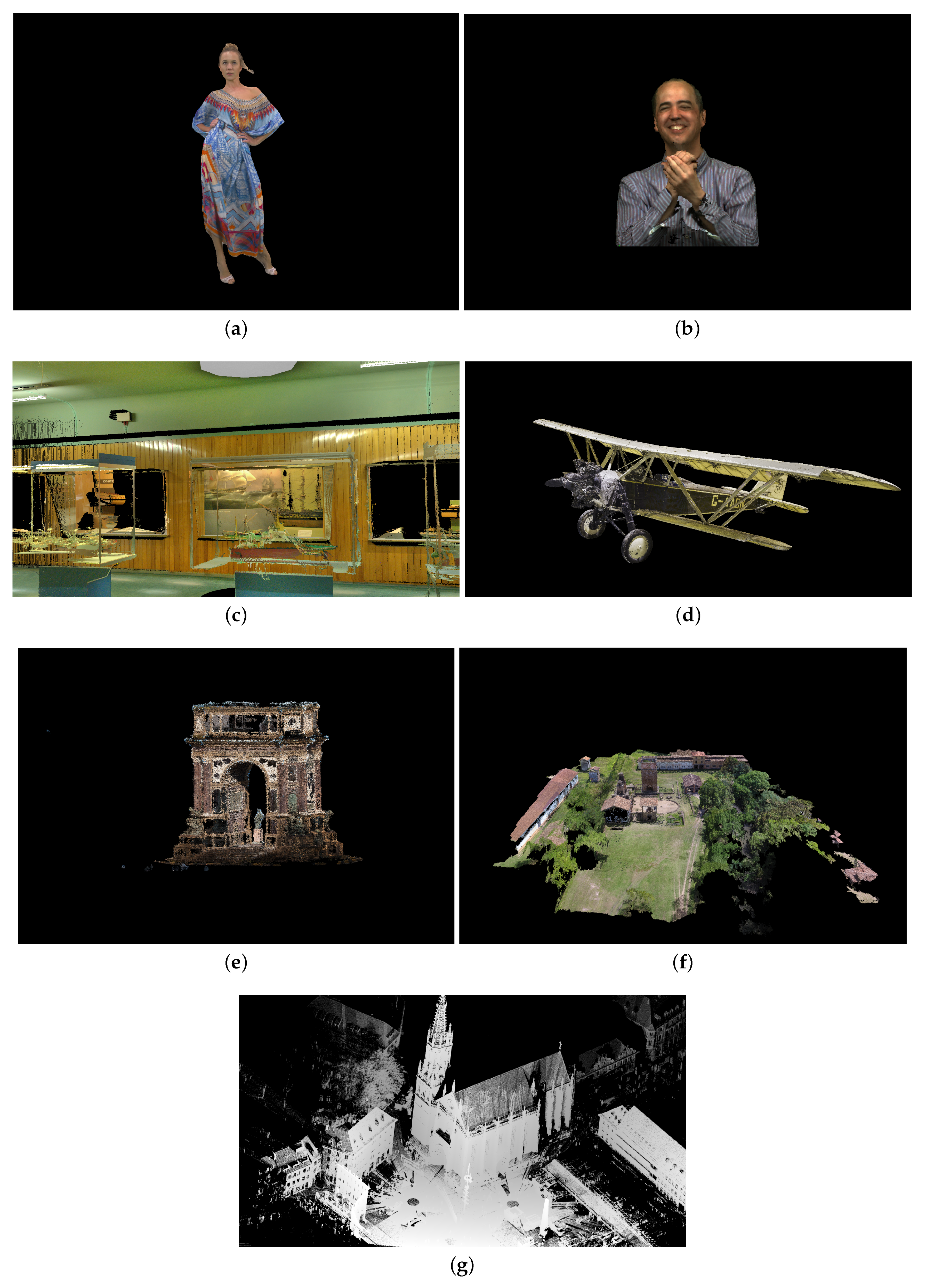
Figure 3 shows one example point cloud from each of those datasets: (a) “8i Voxelized Full Bodies (8iVFB v2)”; (b) “Microsoft Voxelized Upper Bodies”; (c) “ScanLAB Projects: Science Museum Shipping Galleries point cloud data set”; (d) “ScanLAB Projects: Bi-plane point cloud data set”; (e) “UPM Point-cloud data”; (f) “Univ. Sao Paulo Point Cloud dataset”; and (g) 3DTK dataset.

3.2. Subjective Evaluation of Point Clouds

In [30], a novel compression framework is proposed for progressive encoding of time-varying point clouds for 3D immersive and augmented video. Several point cloud coding improvements have been proposed, including generic compression framework, inter-predictive point cloud coding, efficient lossy color attribute coding, progressive decoding, and real-time implementation. Subjective experiments were done, concluding that the proposed compression framework shows similar results, compared to the original reconstructed point clouds.

In [31], the authors presented a new subjective evaluation model for point clouds. Point clouds were degraded by downsampling, geometry noise, and color noise. Subjective quality assessment was performed using procedures defined in ITU-R BT.500 Recommendation. Point clouds were directly shown to the observers, without surface reconstruction, and were displayed using a typical 2D monitor.

Javaheri et al. [32] presented a study on subjective quality assessment of point clouds, firstly degraded with impulse noise and afterwards denoised, using outlier removal and position denoising algorithms. Point clouds were presented to the observer according to the procedures defined in ITU-R BT.500-13, after surface reconstruction. In addition, different objective quality measures for point clouds are calculated and compared with subjective results. Overall, the authors concluded that point2plane measure (using root mean square error as a distance) has better correlation with MOS scores.

In [33], the authors evaluated the subjective quality of rendered point clouds, after compression using two different methods: octree-based and projection-based method. The subjective evaluations were done using crowdsourced workers and expert viewers. Four test stimuli were used, namely “Chapel”, “Church”, “Human”, and “Text”, each with approximately 200 million geometry points. The authors concluded that the projection-based method was preferred, compared to an octree-based method, while having similar compression ratios.

In [34], the authors used PCC-DASH protocol for HTTP adaptive streaming, to create different degradations while streaming scenes that include several dynamic point clouds. Original point clouds were taken from the “8i Voxelized Full Bodies (8iVFB v2)” dataset [28] and were encoded using the V-PCC coder described above, with five different bitrates. Afterwards, objective image and video quality measures were calculated (between generated video sequences from the original and degraded point cloud sequences), with the objective quality estimates showing high correlation with subjective scores.

In [35], the authors presented subjective quality evaluation of point clouds that were encoded directly using V-PCC, or by encoding their mesh representations (in which case both their atlas images and vertices had to be compressed). They also proposed no-reference objective quality measure, depending on the used bitrate and observers’ distance from the screen.

In [36], the authors conducted a detailed investigation of the following aspects for point cloud streaming: encoding, decoding, segmentation, viewport movement patterns, and viewport prediction. In addition, they proposed ViVo, a mobile volumetric video streaming system with three visibility-aware optimizations. ViVo determines the video content to fetch based on how, what, and where a viewer perceives for reducing bandwidth consumption of volumetric video streaming. ViVo showed that, on average, it can save approximately 40% of data usage (up to 80%) with no drop in subjective quality.

4. Objective Measures of Point Cloud Quality

Objective quality measures of visual data such as images and video, and by extension point clouds, are generally used when the subjective assessment may be difficult to conduct [37]. Alternatively, they are also used in different scenarios such as monitoring or optimizing image and video communication systems. Objective quality measures or estimates are computed according to a given algorithm and can be divided in three groups, according to the type of input data required by the algorithm:

• Full-reference (FR) measures: The full original and degraded visual data are used.
• Reduced-reference (RR) measures: Only some features from the original visual data information and degraded visual data information are used.
• No-reference (NR) measures: Only degraded visual data information are used.

Different types of objective measures are presented in Figure 4.

Objective quality measures for point clouds are currently being developed using as paradigms existing quality measures developed for application to image and video, after some modifications to cope with the different representation formats. Generally, those measures can be divided in two main categories:

• measures based on point cloud projections computed on the 2D spaces onto which the points are projected; and
• geometry- and/or attribute-based measures computed on the original 3D space in which the point cloud information is represented.

4.1. Measures Based on Point Cloud Projections

Generally, any point cloud can be projected onto one or several projection planes and afterwards each projection plane can be assessed using any of the existing image quality measures, for example Peak Signal to Noise Ratio (PSNR) or Structural Similarity (SSIM) index [38]. If several projection planes are used giving rise to several projected images, the final score can be calculated as a (weighted) mean of the scores related to each projected image. In [39], the authors described rendering software, which creates voxelized version of point cloud in real time and projects a 3D point cloud onto a 2D plane. Projected images are then compared using existing image quality measures, achieving high correlation with subjective assessment scores.

4.2. Geometry- and/or Attribute-Based Measures

Several objective measures that are based on geometry and attribute information of point clouds have been proposed recently. Generally, two different methods for measuring the geometric distortion have been proposed: point-to-point (p2p) and point-to-plane distances (p2pl) [40]. Firstly, error vector $E_{i,j}$ can be defined as the difference vector between the arbitrary point in the first point cloud $a_j$ to the corresponding point (identified by the nearest neighbor algorithm) in the second point cloud $b_i$. Point-to-point measures operate by computing the distance (error vector length) between each point in one of the point clouds (original or degraded) and the nearest point in the second point cloud (degraded or original). Thereafter, the calculated average squared distance between pairs of points is used as a geometry distortion measure. Distance can be defined differently, with two approaches being used in most cases: Hausdorff distance (Equation (1)) and L2 norm. When L2 norm is used, MSE (Mean Squared Error) (Equation (2)) or RMSE (Root Mean Squared Error) (Equation (3)) can be calculated, between all pairs of closest points. Since this measure can be calculated in two different ways, depending on the order of point clouds (the first point cloud can be the original point cloud and the second one the degraded point cloud and vice versa), the final measure is usually defined as the measure with worse/higher score (called symmetric score).

$$Hau{s}_{p2p}=max(||E_{i,j}{||}_2^2)$$

(1)

$$MS{E}_{p2p}=\frac{1}{n}\sum _{i=1}^n||E_{i,j}{||}_2^2$$

(2)

$$RMS{E}_{p2p}=\sqrt{MS{E}_{p2p}}=\sqrt{\frac{1}{n}\sum _{i=1}^n||E_{i,j}{||}_2^2}$$

(3)

In Equations (1)–(3), $E_{i,j}$ is defined as the difference vector (or point to nearest point vector) between the arbitrary point in the first point cloud $a_j$ to the corresponding nearest point in the second point cloud $b_i$.

However, point-to-point measures do not take into account the form of the implicit surface of which point cloud points are samples. For this reason, a new measure that would successfully represent a surface, called point-to-surface or cloud-to-mesh (c2 m), was studied by Cignoni et al. [41]. Cloud-to-mesh distances approximate surface-to-surface distances, by first sampling one of the point clouds mesh and then computing the point-to-surface distance between every mesh-based sampled point and the other point cloud surface.

Tian et al. [40] proposed alternative geometry-based measure for point clouds called point-to-plane (p2pl). According to this paper (but also in papers described below that use p2pl measure), the proposed measure should obtain higher correlation with subjective assessment, compared to the p2p measure. Basically, p2pl measure can be computed using the following steps:

• Firstly, for each point $a_j$ in the first point cloud, corresponding point $b_i$ in the second point cloud is identified (e.g., by the nearest neighbor algorithm).
• Error vector $E_{i,j}$ is defined (similarly as for the p2p measure) as the difference vector between the arbitrary point in the first point cloud $a_j$ to the corresponding nearest point in the second point cloud $b_i$.
• Unit normal vector $N_j$ is calculated for each point $a_j$ in the first point cloud.
• The error vector is projected onto unit normal vector, by calculating the dot product between error vector $E_{i,j}$ and normal vector $N_j$, obtaining projected error vector.
• Point-to-plane measure is calculated as the mean of the squared magnitudes of all projected error vectors.

Similarly as with the point-to-point measures, MSE, RMSE, or Hausdorff distance can be used in point-to-plane measures. The definition of MSE_p2pl is presented in Equation (4), RMSE_p2pl in Equation (5), and Hausdorff_p2pl in Equation (6).

$$MS{E}_{p2pl}=\frac{1}{n}\sum _{i=1}^n{(<E_{i,j},N_j>)}^2$$

(4)

$$RMS{E}_{p2pl}=\sqrt{MS{E}_{p2pl}}=\sqrt{\frac{1}{n}\sum _{i=1}^n{(<E_{i,j},N_j>)}^2}$$

(5)

$$Hau{s}_{p2pl}=max({(<E_{i,j},N_j>)}^2)$$

(6)

The authors of [40] also introduced a new measure using Peak Signal to Noise Ratio (PSNR), which normalizes the errors related to the peak value of each point cloud. Peak value can be again defined differently. In [40], it is the largest diagonal distance of a bounding box of the point cloud. In MPEG standard [42,43], it is called D1/D2 PSNR measure, which is defined as Equation (7):

$$PSN{R}_{geometry}=10{log}_{10}(\frac{3p^2}{symmetricMS{E}_{geometry}}),p=2^{pr}-1$$

(7)

where p is the signal peak which normalizes the error (it is defined differently for different point clouds): p is the peak constant value and pr the point cloud coordinates precision. In the denominator, symmetricMSE is symmetric MSE explained above (for p2p it is called D1 PSNR and for p2pl it is called D2 PSNR measure). It can be noticed that different scores may be also used in denominator of Equation (7): MSE, RMSE, or Hausdorff based distance.

The MPEG standard [42] proposes attribute-based MSE and PSNR measures.

Because the YUV space is better related to the human perception, the conversion from RGB space to YUV space is carried out. Afterwards, MSE value is separately calculated for each color component. Usually, the maximum value between the obtained MSE values is used to compute symmetric score. The component PSNR is computed according to Equation (8). If the attributes color components for all point clouds have 8 bit depth, then the peak value p used in Equation (8) is 255. Final global MSE or PSNR is calculated averaging the individual (Y, U, and V) MSEs or PSNRs using a weight of 6/8 for luminance (Y) and 1/8 to both chrominances (U and V).

$$PSN{R}_{attribute}=10{log}_{10}(\frac{p^2}{symmetricMS{E}_{attribute}})$$

(8)

In [44], the authors proposed a new full-reference objective quality measure for point clouds, called PCQM. The measure uses information from both geometry-based and attribute-based point cloud features and calculates the final score as a weighted combination of several proposed features. PCQM was tested on the MPEG dataset [27] with three codecs (Octree pruning, G-PCC coder, and V-PCC coder), each with three quality levels, and obtained highest correlation with subjective scores, among all tested objective measures.

Javaheri et al. [32] tested p2p and p2pl objective measures using point clouds compressed with octree pruning and graph-based compression. They concluded that p2pl measure obtains higher correlation.

5. Common Methods for the Analysis and Presentation of the Results from Subjective Assessment

To be able to compare subjective MOS grades between different laboratories, or to compare subjective Mean opinion score (MOS) grades with different objective quality estimators, different correlation measures can be used. The most common are Pearson’s Correlation Coefficient (Pcc), Spearman’s Rank Order Correlation Coefficient (SROCC), and Kendall’s Rank Order Correlation Coefficient (KROCC). Pearson’s correlation coefficient measures the agreement between two variables x and y observed through n samples and is defined in Equation (9)

$$PC{C}_{xy}=\frac{{\sum }_{i=1}^n(x_i-\overline{x})(y_i-\overline{y})}{\sqrt{{\sum }_{i=1}^n{(x_i-\overline{x})}^2}\sqrt{{\sum }_{i=1}^n{(x_i-\overline{x})}^2}}=\frac{{\sum }_{i=1}^n(x_i-\overline{x})(y_i-\overline{y})}{(n-1)s_x{s}_y}$$

(9)

where $x_i$ and $y_i$ are sample values (e.g., x can be MOS values from the first laboratory, while y can be MOS values from the second laboratory; alternatively, x can be MOS values and y objective scores after nonlinear regression), whereas $\overline{x}$ and $\overline{y}$ are sample mean and $s_x$ and $s_y$ are corrected sample standard deviations from x and y. Spearman’s rank order correlation coefficient [45] is another useful correlation measure to compare ordinal association between two variables. Unlike PCC that calculates linearity, SROCC calculates monotonicity of the relationship between them. To calculate SROCC, each variable has to be ranked firstly (for all tied ranks, mean rank is assigned) and afterwards PCC can be calculated over the ranked variables. Kendall’s rank order correlation coefficient [46] is also a correlation measure that, similarly to SROCC, calculates ordinal association between two variables. After both variables are ranked, pair observations over them need to be found: concordant pairs, discordant pairs, and possibly tied pairs (neither concordant nor discordant). Generally, three types of KROCC are defined, usually called ${\tau }_a$, ${\tau }_b$, and ${\tau }_c$. While ${\tau }_a$ does not take into account tied pairs, ${\tau }_b$ and ${\tau }_c$ do. In addition, ${\tau }_b$ is usually used for variables that have the same number of possible values (before ranking), while ${\tau }_c$ also takes into account different number of possible values. We use ${\tau }_b$ coefficient below.

When using PCC, usually a nonlinear regression function is used to better fit objective measures with subjective MOS scores. For comparison between different MOS scores (e.g., to compare results from different laboratories), linear regression can also be used. Equations (10)–(13) show some common fitting functions used in the context of visual stimuli quality evaluations.

$$C_1\left(z\right)=b_1(\frac{1}{2}-\frac{1}{1+e^{b_2(z-b_3)}})+b_{4}z+b_5$$

(10)

$$C_2(z)=\frac{b_1-b_2}{1+e^{(z-b_3)/b_4}}$$

(11)

$$C_3(z)=b_1{z}^3+b_2{z}^2+b_{3}z+b_4$$

(12)

$$C_4(z)=b_{1}z+b_2$$

(13)

Equations (10) and (11) describe logistic fittings and were used by Sheikh and Bovik [47] and Larson and Chandler [48], respectively, while Equations (12) and (13) describe cubic and linear fittings.

An important step in the processing of the MOS scores is outlier detection, used, e.g., in the DSIS subjective assessment method described in ITU-R BT.500-14 [24]. Firstly, according to Equation (14), kurtosis ${\beta }_i$ and standard deviation $s_i$ are calculated for all video sequences $iϵ\{1,n\}$. Afterwards, a screening rejection algorithm is applied, as described in (15).

$$\begin{array}{c}\hfill {\beta }_i=\frac{\frac{1}{n}{\sum }_{i=1}^n{(x_{i,j}-\overline{x_i})}^4}{{(\frac{1}{n}{\sum }_{i=1}^n{(x_{i,j}-\overline{x_i})}^2)}^2}\\ \hfill s_i=\sqrt{\frac{1}{n-1}\sum _{i=1}^n{(x_{i,j}-\overline{x_i})}^2}\end{array}$$

(14)

$$\begin{array}{cc}\hfill & \mathrm{for}\mathrm{every}\mathrm{video}\mathrm{sequence}iϵ\{1,n\}\hfill \\ \hfill & \mathrm{for}\mathrm{every}\mathrm{observer}j\hfill \\ \hfill & \mathrm{if}2\le {\beta }_i\le 4\hfill \\ \hfill & \mathrm{if}{x}_{i,j}\ge \overline{x_i}+2s_i\mathrm{then}{P}_{i,j}=P_{i,j}+1\hfill \\ \hfill & \mathrm{if}{x}_{i,j}\le \overline{x_i}-2s_i\mathrm{then}{Q}_{i,j}=Q_{i,j}+1\hfill \\ \hfill & \mathrm{else}\hfill \\ \hfill & \mathrm{if}{x}_{i,j}\ge \overline{x_i}+\sqrt{20}{s}_i\mathrm{then}{P}_{i,j}=P_{i,j}+1\hfill \\ \hfill & \mathrm{if}{x}_{i,j}\le \overline{x_i}-\sqrt{20}{s}_i\mathrm{then}{Q}_{i,j}=Q_{i,j}+1\hfill \\ \hfill & \hfill \\ \hfill & \mathrm{for}\mathrm{every}\mathrm{observer}\mathrm{j}\hfill \\ \hfill & \mathrm{if}\frac{P_{i,j}+Q_{i,j}}{n}>0.05\mathrm{and}|\frac{P_{i,j}-Q_{i,j}}{P_{i,j}+Q_{i,j}}|<0.3\mathrm{then}\mathrm{reject}\mathrm{observer}\mathrm{j}\hfill \end{array}$$

(15)

Another goodness of fit measure is root mean squared error (RMSE), defined by Equation (16)

$$RMSE=\sqrt{\frac{1}{n}\sum _{i=1}^n{(fit\left(x_i\right)-y_i)}^2}$$

(16)

Outlier ratio (OR) is also used for comparison between two sets of grades, e.g., from two different laboratories, and can be defined as a number of grades that satisfy Equation (17).

$$|fit\left(x_i\right)-y_i|>=\frac{1}{2}(C{I}_{x,i}+C{I}_{y,i})$$

(17)

In Equation (17), x and y are MOS values from two different laboratories, while CI is defined as Equation (18)

$$\begin{array}{c}\hfill C{I}_{x,i}=t(m-1)\frac{s_{x,i}}{\sqrt{m}}\\ \hfill C{I}_{y,i}=t(m-1)\frac{s_{y,i}}{\sqrt{m}}\end{array}$$

(18)

where m is a number of gathered scores per video sequence, t(m − 1) is Student’s t inverse cumulative distribution function (defined for the 95% confidence interval below, two-tailed test) with $m-1$ degrees of freedom, and $s_{x,i}$ and $s_{y,i}$ are standard deviations for all gathered scores for video sequence i.

The outlier ratio (OR) can also be used to compare MOS scores and objective scores, by counting the number of grades that satisfy Equation (19)

$$|fit\left(x_i\right)-y_i|>=2s_i$$

(19)

where $x_i$ represents objective score for video sequence i, $y_i$ represents MOS score for video sequence i, and $s_i$ is the standard deviation for all gathered subjective scores for video sequence i.

6. Point Cloud Subjective and Objective Quality Evaluation—A Case Study

In this section, we describe a case study on the evaluation of point clouds subjective and objective quality. This study involved two research laboratories, one in the University of Coimbra (UC), Portugal and the other in University North (UNIN), Croatia. The study included collection of subjective quality scores using observers in both laboratories. The scores were evaluated calculating correlations between the scores collected at UC and UNIN. Further, correlations between objective measures and subjective MOS grades were computed both for UC and UNIN scores.

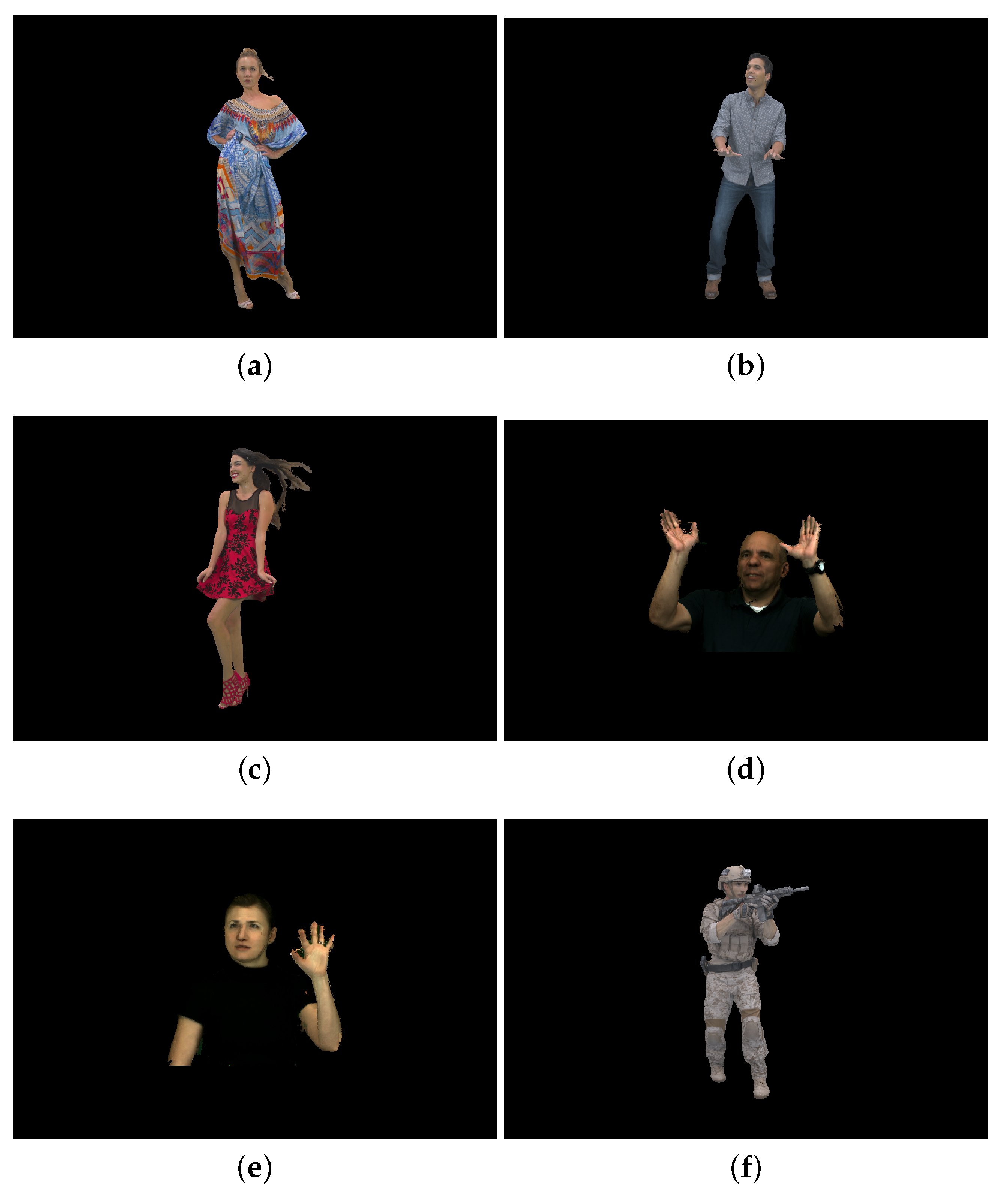
Part of these results is also presented in [49]. The objective quality measures were computed according to Tian et al. [40]. Figure 5 Illustrates the point clouds used in the study. All point clouds are publicly available in JPEG Pleno Point Cloud datasets [27,28].

6.1. Inter-Laboratory Correlation Results

The details of the subjective evaluation are described in [49]. Concisely, six point clouds were used for subjective assessment, each compressed with two MPEG codecs (G-PCC Oct-tree, G-PCC Tri-soup, and V-PCC), each with five compression levels, adjusted to represent diverse visual impairments. 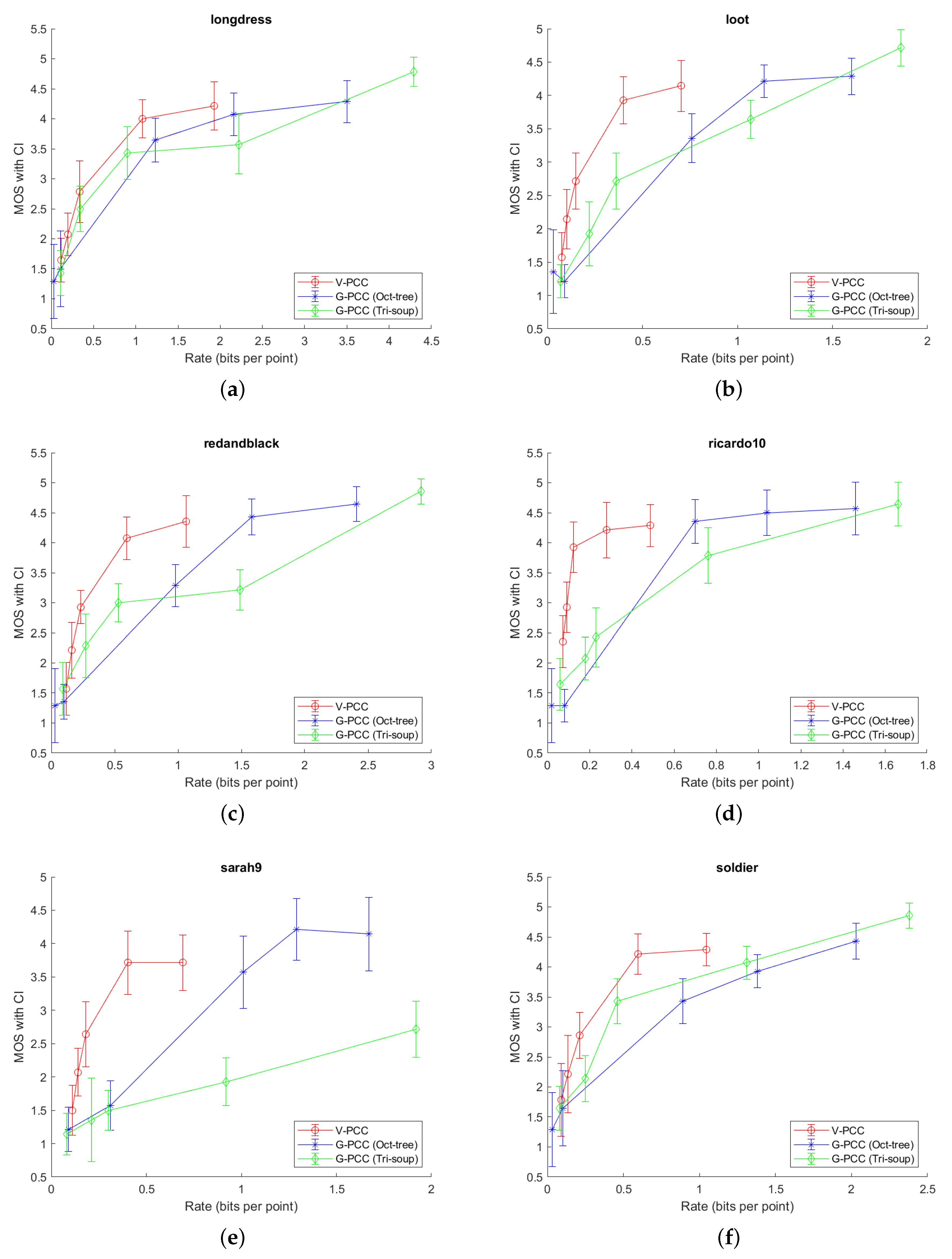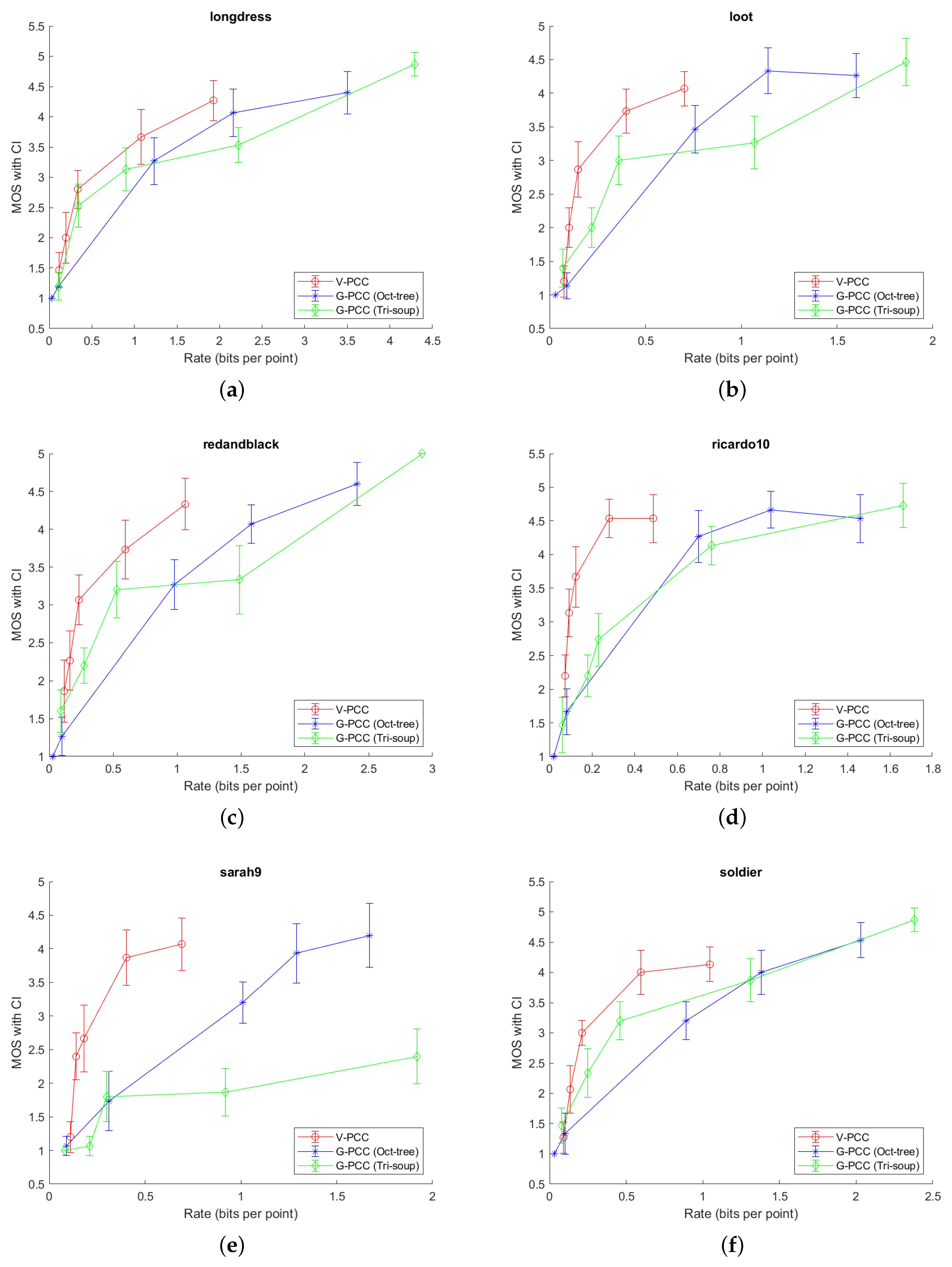Target bitrates were chosen similarly to the MPEG point cloud coding Common Test Conditions (CTC) [42], with some differences explained in [49]. DSIS evaluation protocol was used, simultaneously showing original and degraded point cloud and a five-point rating was adopted (very annoying; annoying; slightly annoying; perceptible, but not annoying; and imperceptible). Overall, 96 point clouds were used in the subjective evaluation, including six hidden reference (original) point clouds (six point clouds, three different encoder types, and five levels of compression per encoder plus the six originals equals 6 × 3 × 5 + 6 = 96 point clouds). Each point cloud was rotated around its vertical axis by 0.5 per frame, giving overall 720 frames per tested point cloud. All frames were packed in video sequences with 12 s duration and 60 fps (12 × 60 = 720 frames), using FFmpeg and H.264/AVC compression with lower constant rate factor (crf), producing near lossless quality. Finally, video sequences were presented to the observers using customized MPV video player, with overall duration of 96 × 12 = 1152 s or around 20 min, in addition to the time needed to enter the score. Sequences were shown to the observers randomly, but taking into account that the same content is not shown consecutively. Equipment characteristics and observers demographic statistics are presented in

Table 1. Equipment information, observers statistics and outliers.

	UC	UNIN
Monitor	Sony KD-49X8005C	Sony KD-55X8505C
Screen Diagonal	49″	55″
Resolution	3840 × 2160 pixels	3840 × 2160 pixels
Viewing distance	1.8 m ± 30 cm	1.5 m ± 15 cm
Male Observers	7	10
Female Observers	8	5
Overall	15	15
Age range (years)	18–54	19–59
Average age (years)	28	29
Number of outliers	0	0

.

Outlier rejection was performed according to Equation (15) and no outliers were found. Afterwards, MOS scores and CI were calculated according to Equation (18). The results for UC and UNIN are presented in Figure 6 and Figure 7. Outlier numbers are presented in Table 1 too.

In Figure 6 and Figure 7, it can be generally seen that V-PCC coder outperforms G-PCC for all tested point clouds, or, alternatively, needs less bits per point (bpp) for the similar MOS score. However, in this experiment, we tested only one type of content, which may be better suited for V-PCC encoder. A different content type (e.g., in sensor-based navigation) might obtain better results with different encoder. In addition, it can be seen that Longdress point cloud needs more bpp, to obtain higher MOS score, compared to the all other point clouds. Redandblack and soldier point clouds are in the middle, when comparing needed bpp and higher MOS. Loot, Ricardo10 and Sarah9 need less bpp to obtain higher MOS score, when comparing with the other three point clouds. This can be explained because of the different complexity of each compressed point cloud. Longdress, Redanblack and Soldier have more details, comparing to, e.g., Ricardo10 and Sarah9 point clouds, which can be also seen in Figure 5. Another problem with point clouds Ricardo10 and Sarah9 may be the noise which is present even in the original point clouds (Figure 5); thus, observers might not notice finer differences when comparing them with (not highly) compressed point clouds.

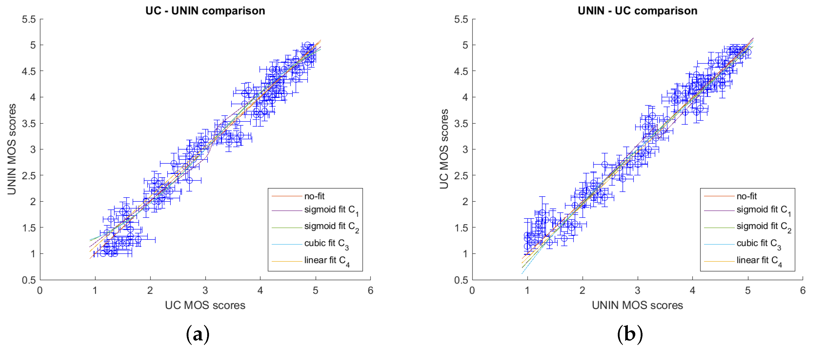
Afterwards, a comparison between laboratories was performed computing correlations for the pairs UC-UNIN and UNIN-UC using Equations (10)–(13) as fitting functions. Figure 8 presents the comparison between laboratories in graphical form, while

Table 2. Inter-laboratory correlation, UC-UNIN.

	C1	C2	C3	C4	No Fit
PCC	0.9892	0.9886	0.9886	0.9864	0.9864
SROCC	0.9823	0.9823	0.9823	0.9823	0.9823
KROCC	0.8992	0.8992	0.8992	0.8992	0.8992
RMSE	0.1832	0.1883	0.1886	0.2057	0.2186
OR	0.0938	0.0417	0.0729	0.0625	0.0729

and

Table 3. Inter-laboratory correlation, UNIN-UC.

	C1	C2	C3	C4	No Fit
PCC	0.9878	0.9868	0.9870	0.9864	0.9864
SROCC	0.9831	0.9823	0.9823	0.9823	0.9823
KROCC	0.9032	0.8992	0.8992	0.8992	0.8992
RMSE	0.2001	0.2079	0.2062	0.2111	0.2186
OR	0.1042	0.0833	0.0938	0.0833	0.0729

present correlation results using PCC ((9)), SROCC, KROCC, RMSE ((16)), and OR ((17)). From the results, it can be seen that correlation between both laboratories is high, meaning that the subjective assessment was correctly performed.

6.2. Objective Quality Measures and Correlation with MOS Scores

In this section, we present correlation results of the subjective scores from UC and UNIN laboratories as well as with different objective measures described above. The results are calculated using only 84 MOS scores: six were skipped because they belonged to the original undegraded reference point clouds and six were encoded using G-PCC coder with parameters for lossless geometry.

Agreements between scores were calculated using PCC ((9)), SROCC, KROCC, RMSE ((16)), and OR ((19)). PCC was calculated after nonlinear regression using C₁ ((10)), C₂ ((11)), and C₃ ((12)) functions. The RMSE_p2p measure was used as square root of MSE (Equation (3)), while Hausdorff_p2p distance used (1). RMSE_p2pl was calculated as Equation (5) and Hausdorff_p2pl as Equation (6). 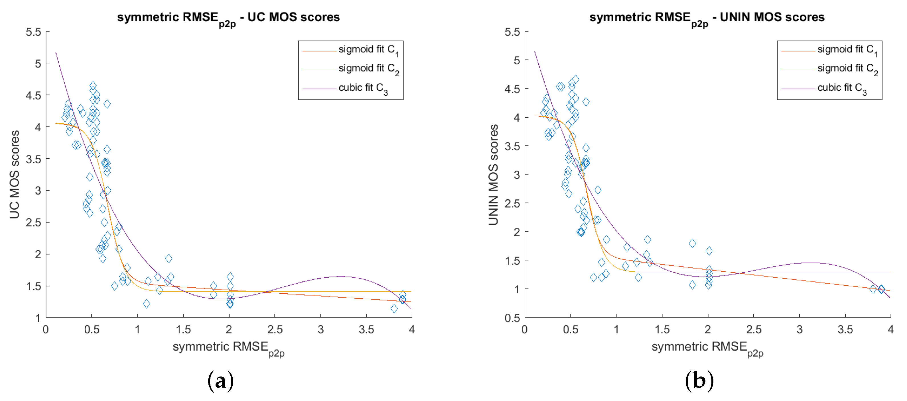PSNR values were calculated similarly to Equation (7), but with $p^2$ in numerator and p value being defined as the largest diagonal distance of a bounding box of the point cloud, as defined in [40]. From the results in

Table 4. PCC, SROCC, KROCC, RMSE and OR between UC and different objective measures (best values are bolded).

	RMSEp2p	PSNRRMSE,p2p	RMSEp2pl	PSNRRMSE,p2pl	Hausp2p	PSNRHaus,p2p	Hausp2pl	PSNRHaus,p2pl
PCC_C1	0.8705	0.6047	0.9426	0.6666	0.6038	0.5148	0.6215	0.4907
PCC_C2	0.8694	0.5722	0.9418	0.6016	0.5723	0.4844	0.5722	0.4699
PCC_C3	0.8400	0.5599	0.9218	0.5832	0.4604	0.4918	0.5573	0.4717
SROCC	0.8207	0.5522	0.9172	0.5752	0.4532	0.4491	0.5391	0.4314
KROCC	0.6265	0.3933	0.7379	0.4281	0.3268	0.3220	0.3896	0.3153
RMSE_C1	0.5684	0.9197	0.3856	0.8608	0.9204	0.9899	0.9047	1.0061
OR_C1	0.0238	0.2143	0	0.1667	0.2024	0.1786	0.1905	0.2143

and

Table 5. PCC, SROCC, KROCC, RMSE and OR between UC and different objective measures (best values are bolded).

	RMSEp2p	PSNRRMSE,p2p	RMSEp2pl	PSNRRMSE,p2pl	Hausp2p	PSNRHaus,p2p	Hausp2pl	PSNRHaus,p2pl
PCC_C1	0.8803	0.6542	0.9423	0.7038	0.5721	0.5071	0.5923	0.5115
PCC_C2	0.8763	0.6181	0.9397	0.6424	0.5504	0.4782	0.5500	0.4989
PCC_C3	0.8446	0.6129	0.9225	0.6354	0.4161	0.4828	0.5262	0.4795
SROCC	0.8212	0.5888	0.9194	0.6196	0.4187	0.4755	0.5379	0.4726
KROCC	0.6205	0.4298	0.7451	0.4715	0.3055	0.3325	0.3954	0.3391
RMSE_C1	0.5683	0.9059	0.4011	0.8510	0.9824	1.0324	0.9651	1.0293
OR_C1	0.1429	0.2857	0.0714	0.2738	0.3333	0.3333	0.2976	0.3452

and Figure 9, it can be seen that the best performing objective measure is RMSE_p2pl, in both UC and UNIN laboratories. The second best measure is RMSE_p2p, also in both tested laboratories (Table 4 and Table 5 and Figure 10). Other objective measures have lower correlation scores.

When comparing different nonlinear regression functions used in experiments, best results were obtained using C₁ as fitting function for PCC calculation, in both UC and UNIN laboratories. The second best is C₂, also in both laboratories, being only slightly lower than case with C₁. When comparing RMSE_p2p with PSNR_RMSE,p2p and RMSE_p2pl with PSNR_RMSE,p2pl, it can be noticed that PSNR obtained lower correlation than RMSE. PSNR was calculated using p value defined as the largest diagonal distance of a bounding box of the point cloud.

PSNR achieves higher correlation if it is calculated as defined in Equation (7), e.g., with $3p^2$ in numerator and p value being defined as the peak constant value (e.g., 511 for 9-bit precision, for Sarah9 point cloud and 1023 for 10-bit precision for other tested point clouds;

Table 6. PCC, SROCC, KROCC, RMSE and OR between UC, UNIN and differently calculated PSNR measure.

	UC		UNIN
	PSNRRMSE,p2p	PSNRRMSE,p2pl	PSNRRMSE,p2p	PSNRRMSE,p2pl
PCC_C1	0.8712	0.9440	0.8802	0.9426
PCC_C2	0.8693	0.9439	0.8768	0.9421
PCC_C3	0.8421	0.9279	0.8478	0.9290
SROCC	0.8207	0.9172	0.8212	0.9194
KROCC	0.6265	0.7379	0.6205	0.7451
RMSE_C1	0.5669	0.3810	0.5684	0.4000
OR_C1	0.0238	0	0.1429	0.0714

). In this case, RMSE and PSNR have similar correlation scores, e.g., PCC_C₁ between PSNR_RMSE,p2pl and MOS is around 0.94 and PCC_C₁ between PSNR_RMSE,p2p and MOS is around 0.87, in both UC and UNIN laboratories. In addition, best results were obtained using C₁ as fitting function for PCC calculation, in both UC and UNIN laboratories, while C₂ produces slightly lower PCC correlation between PSNR and MOS.

7. Conclusions

In this paper, we present a general framework for subjective evaluation of point clouds, as well as currently proposed objective metrics for point cloud quality measurement. Afterwards, we present a case study using results from subjective evaluations of point clouds performed in a collaboration between two international laboratories at the University of Coimbra in Portugal and the University North in Croatia. The results as well as their analysis show that the correlation between both laboratories is high, meaning that the subjective assessments were performed correctly. When comparing different geometry-based objective measures, the objective quality estimates that were found to be better correlated with subjective scores were obtained using a symmetric RMSE_p2pl measure, in both laboratories, while second best was RMSE_p2p measure, also for both laboratories subjective scores sets.

In view of the results obtained, it is clear that new objective metrics should be developed aiming at better correlation with subjective grades. Due to the joint importance of geometry and attribute (color) information, new measures should be based on these two sets of point cloud information. It is also clear that new point cloud test datasets should be compiled, representing different objects and diverse environments, as current datasets are mostly constituted by small objects and a few human figures. These activities will be the focus of future research by the authors.