Mapping Landslide Susceptibility Using Machine Learning Algorithms and GIS: A Case Study in Shexian County, Anhui Province, China


Abstract
:1. Introduction
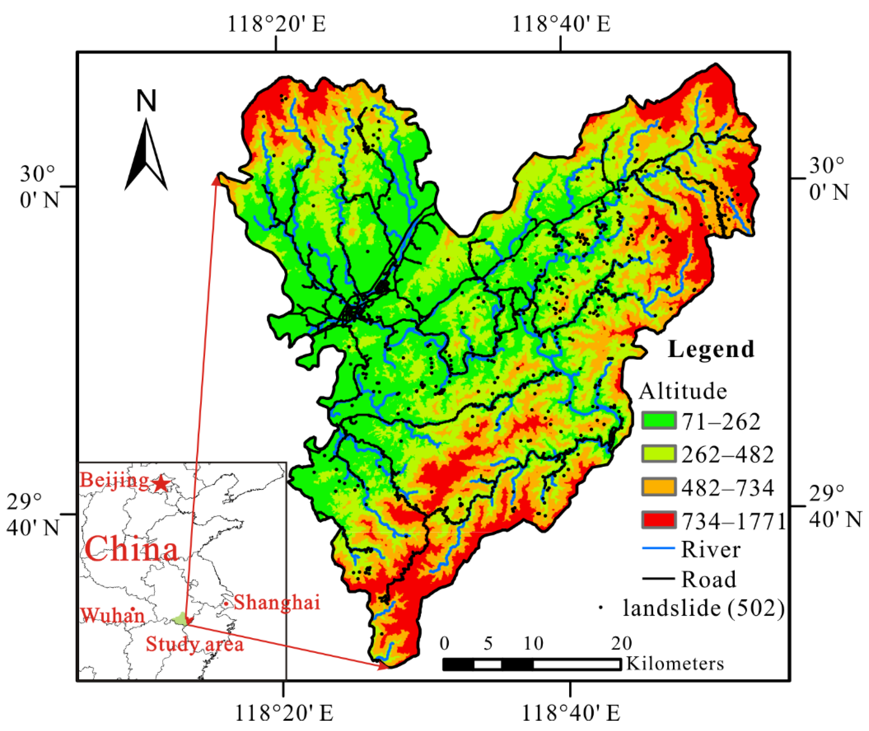
2. Study Area
3. Data
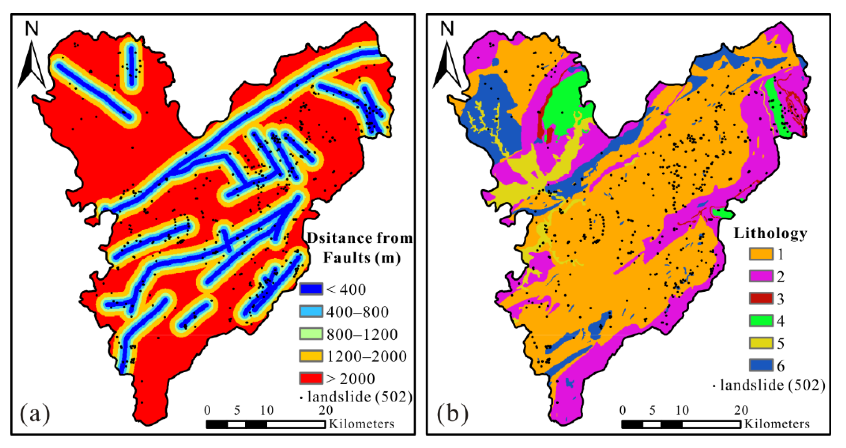
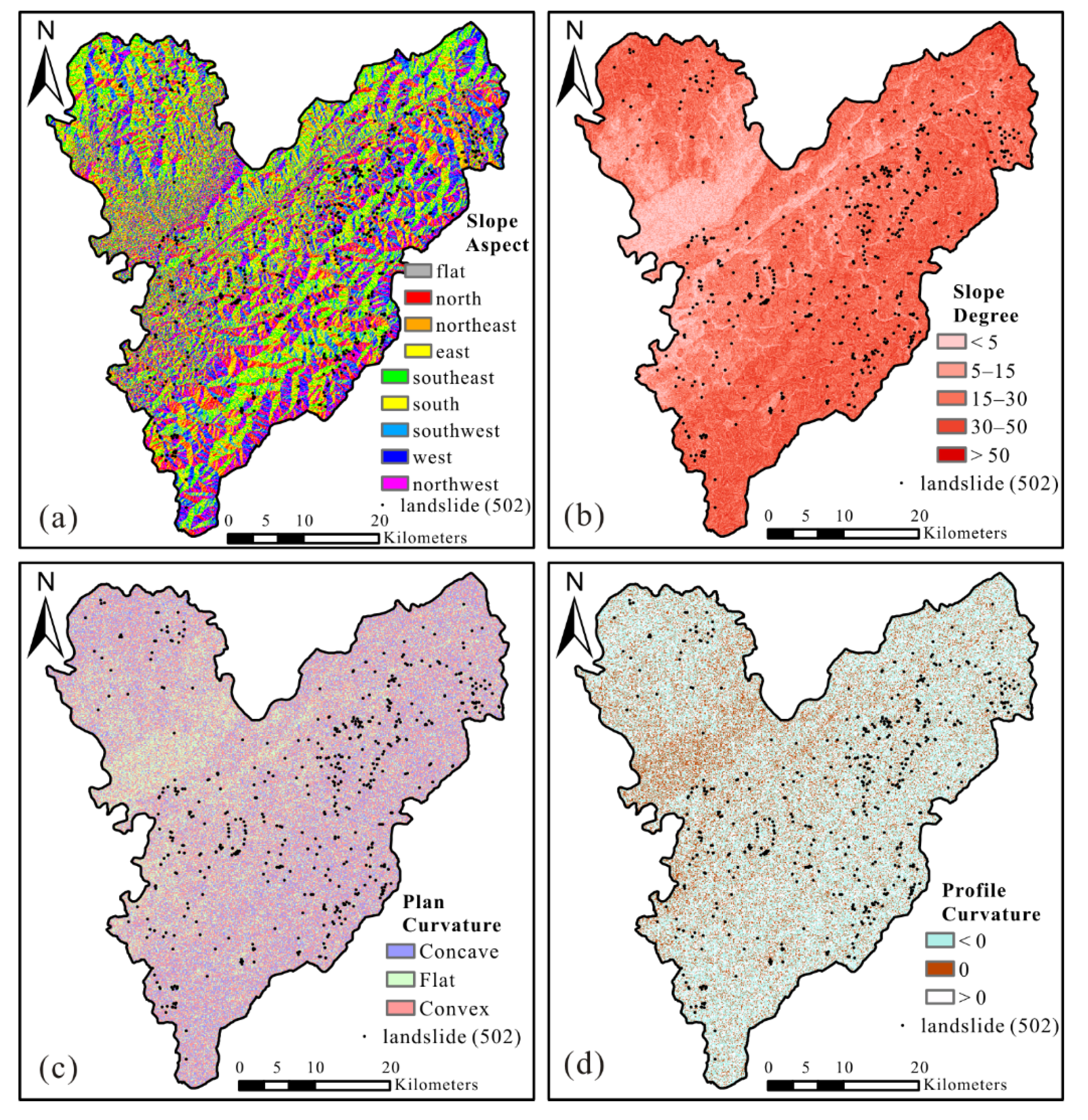
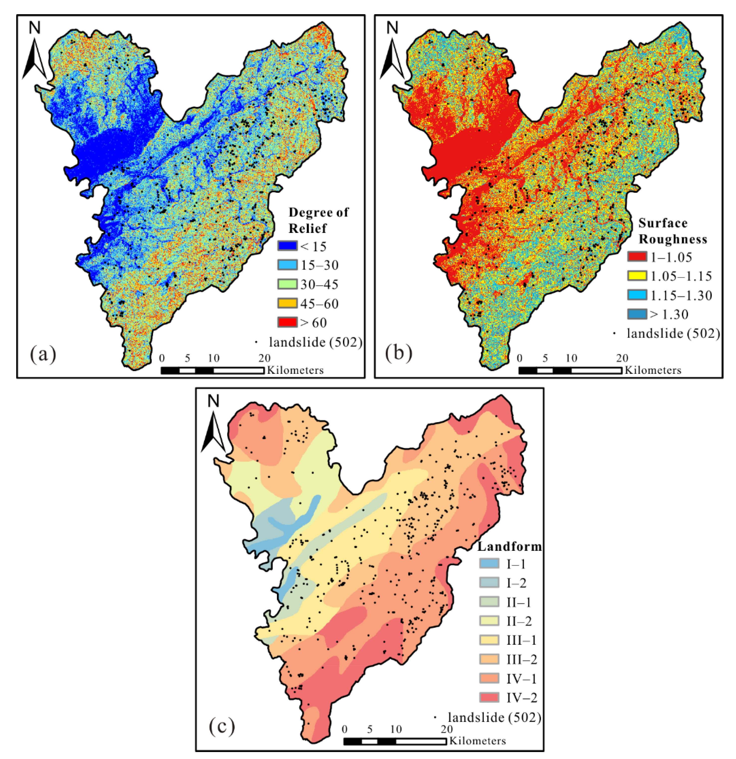
3.1. Topographical and Geological Factors
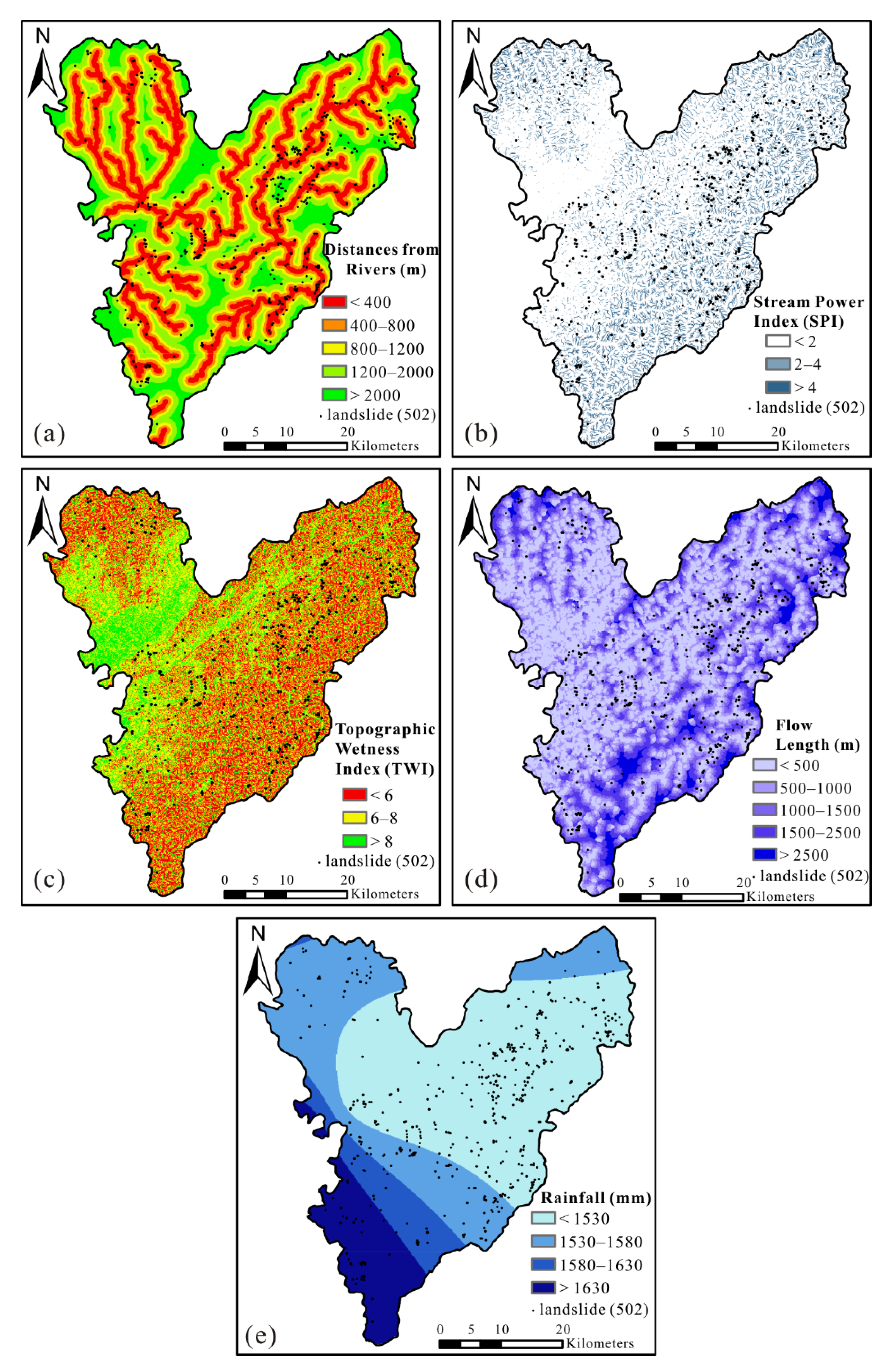
3.2. Hydrological Factors
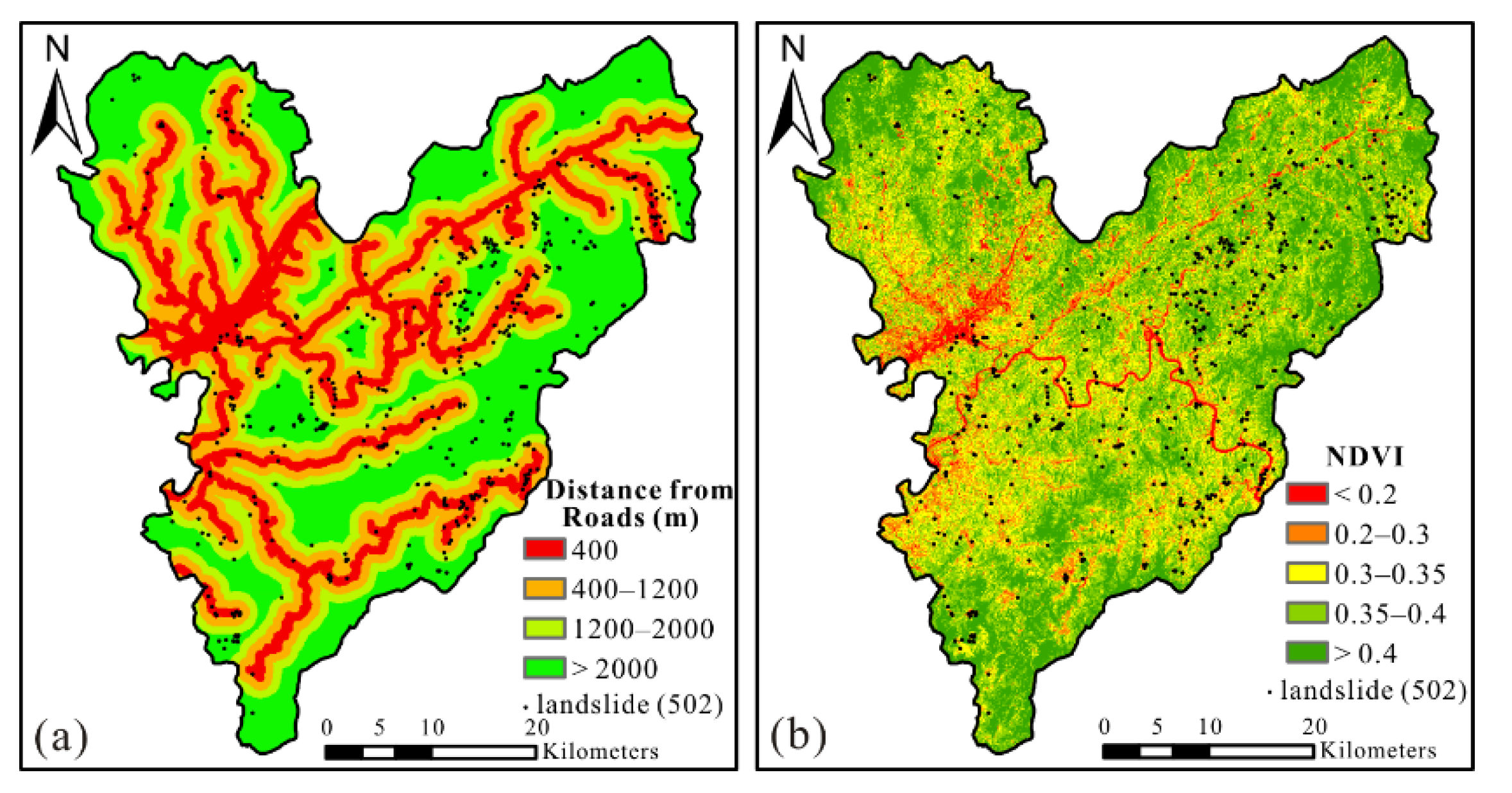
3.3. Other Factors
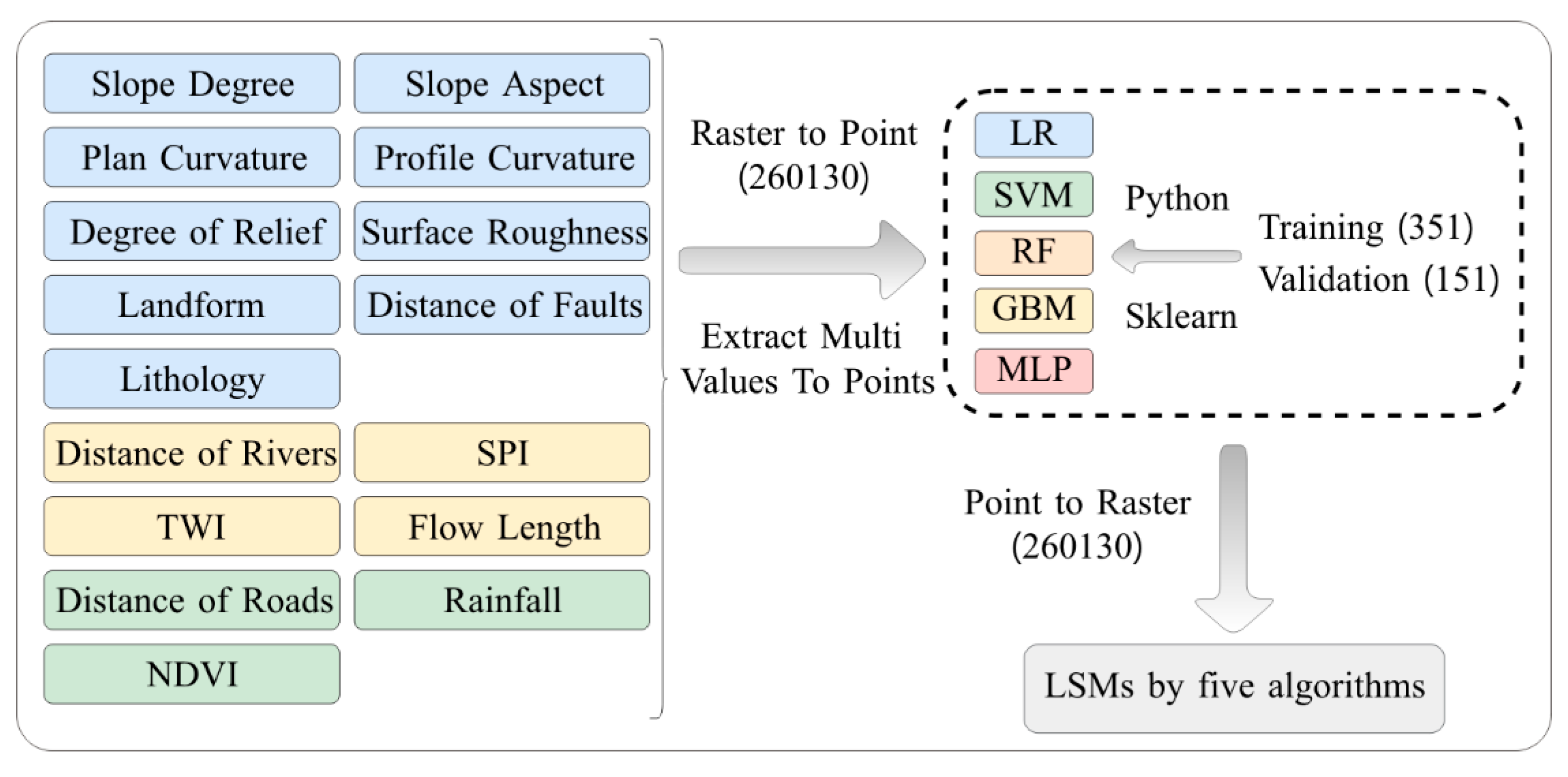
4. Methodology
4.1. Logistic Regression (LR)
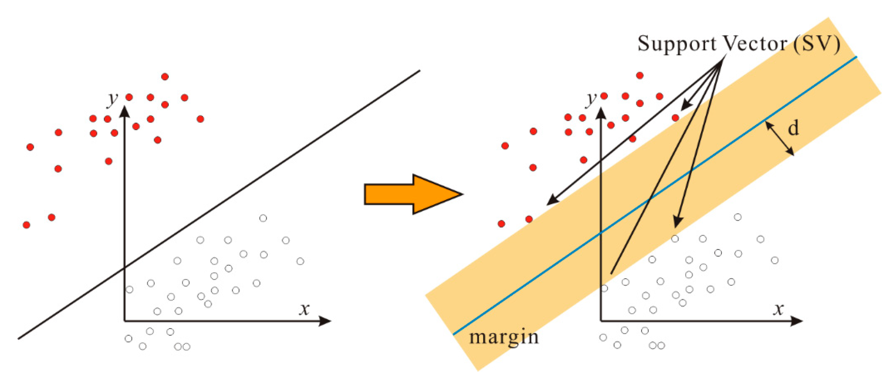
4.2. Support Vector Machine (SVM)
4.3. Random Forest (RF)
4.4. Gradient Boosting Machine (GBM)
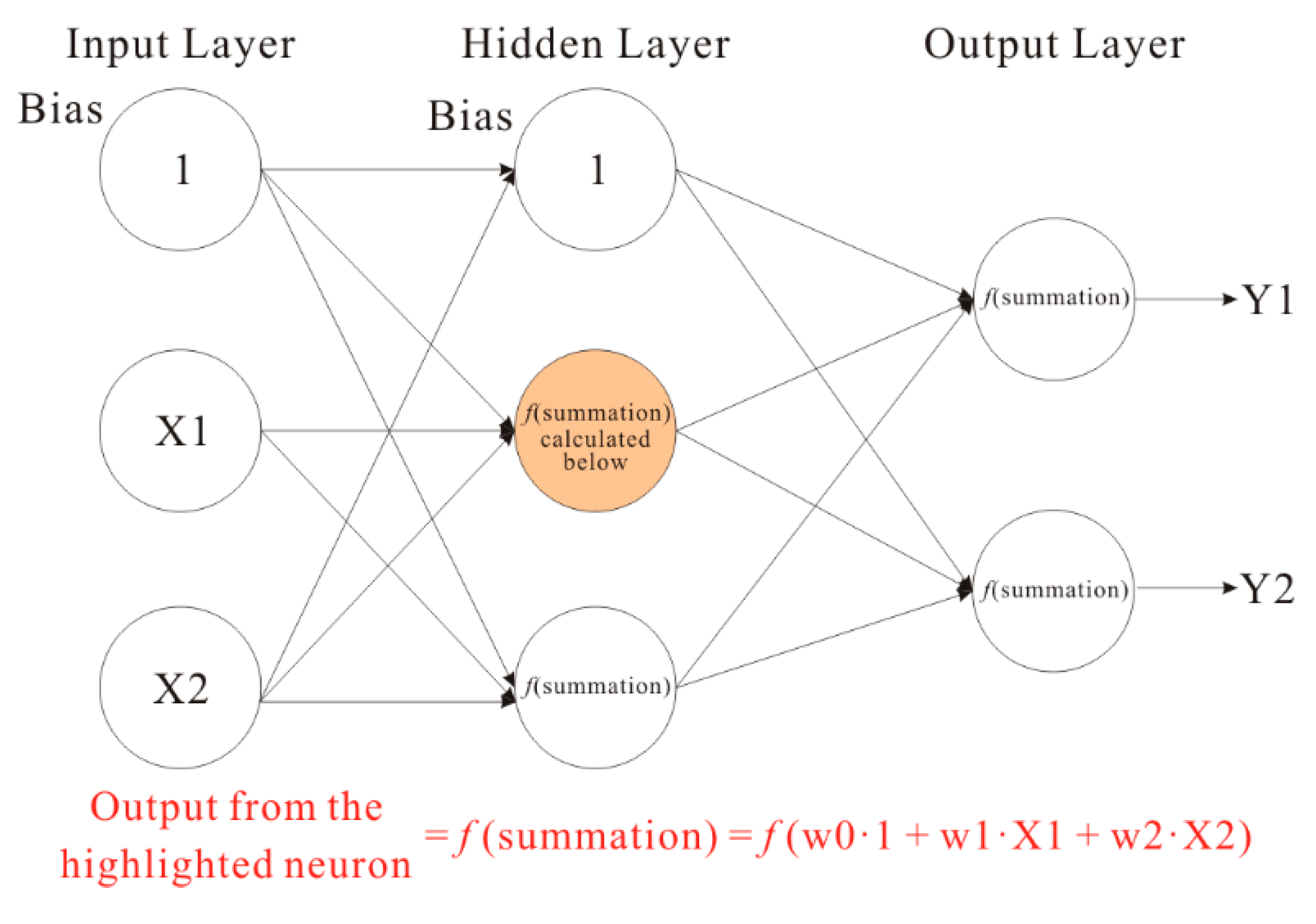
4.5. Multilayer Perceptron (MLP)
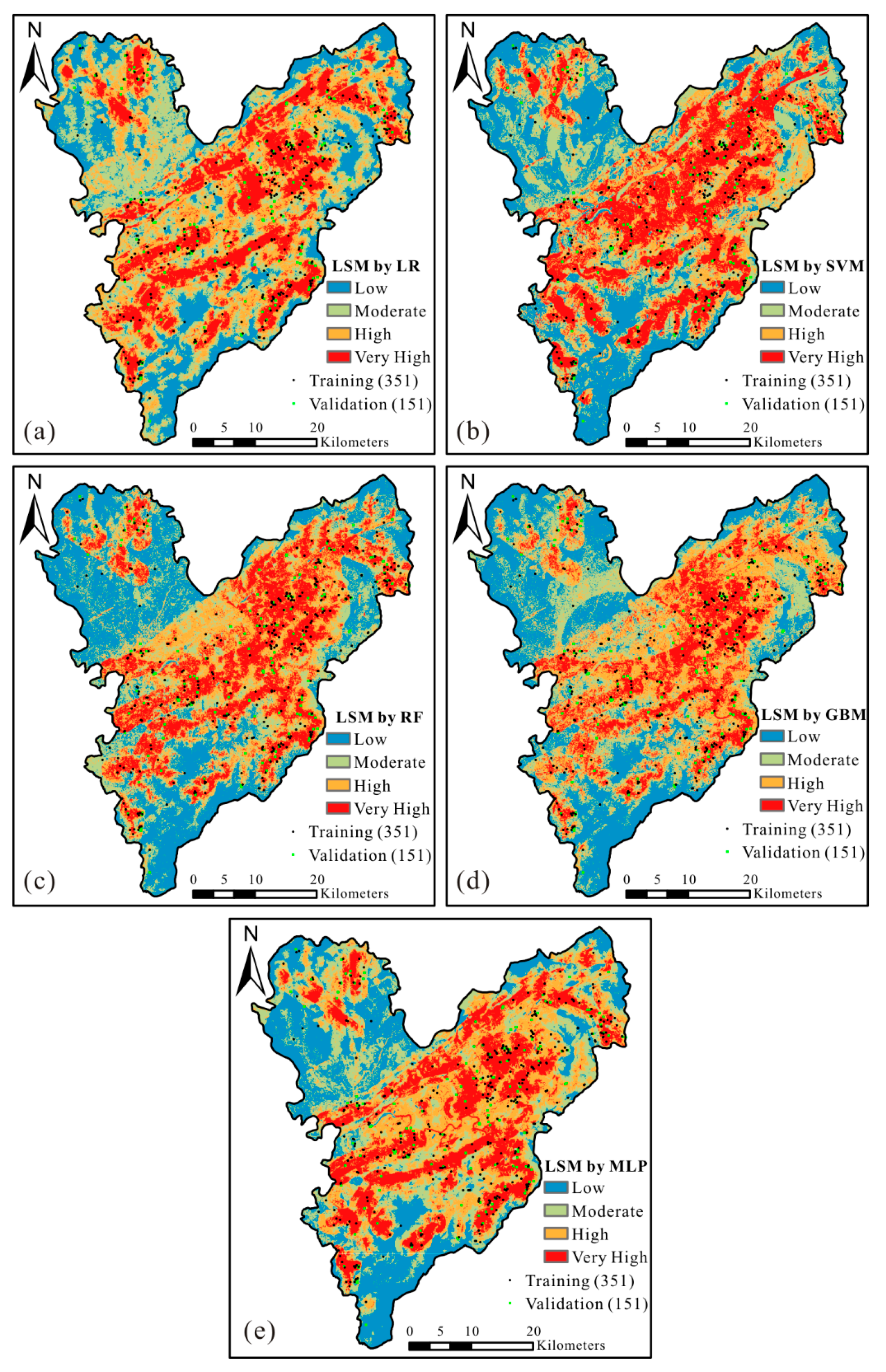
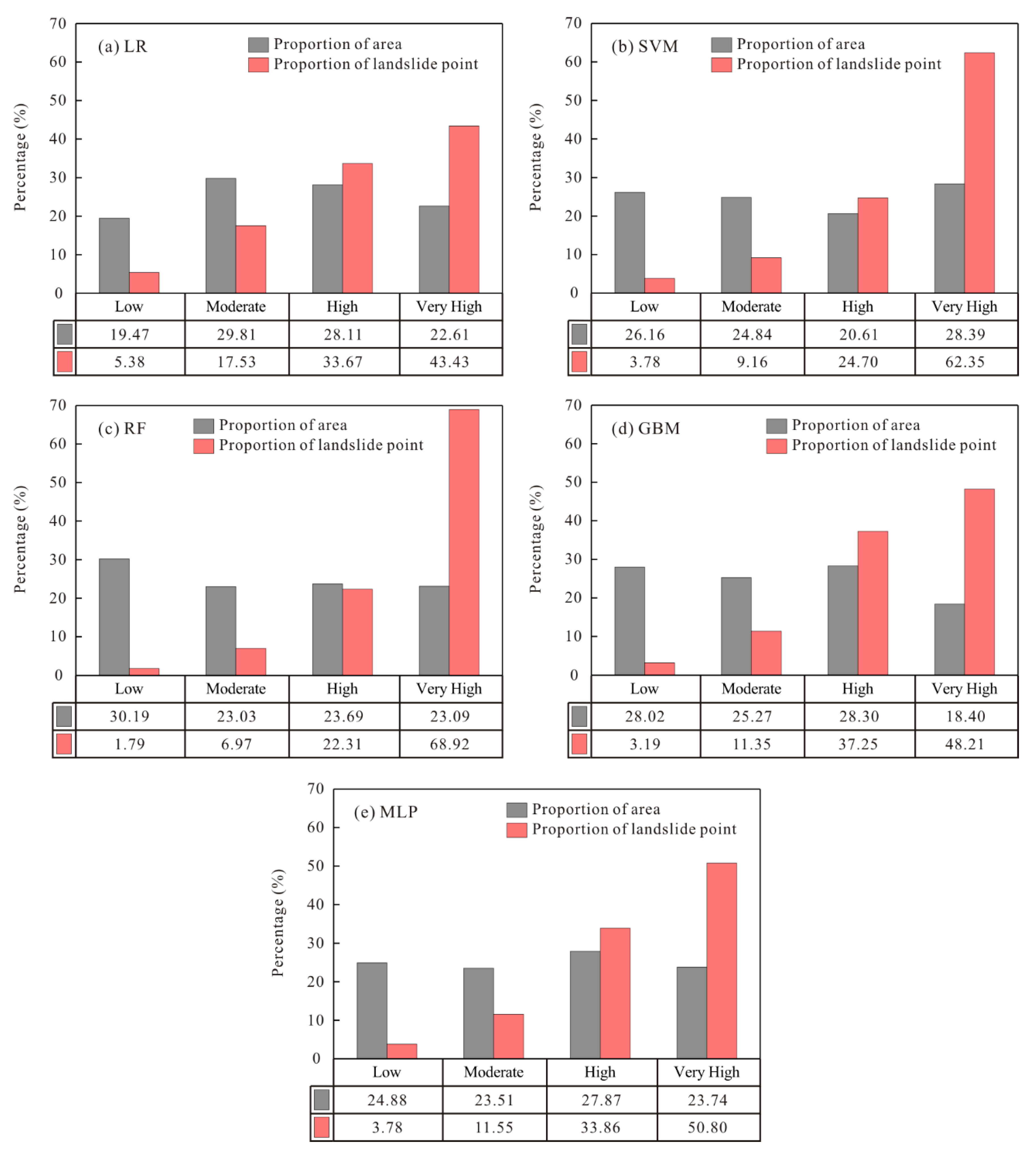
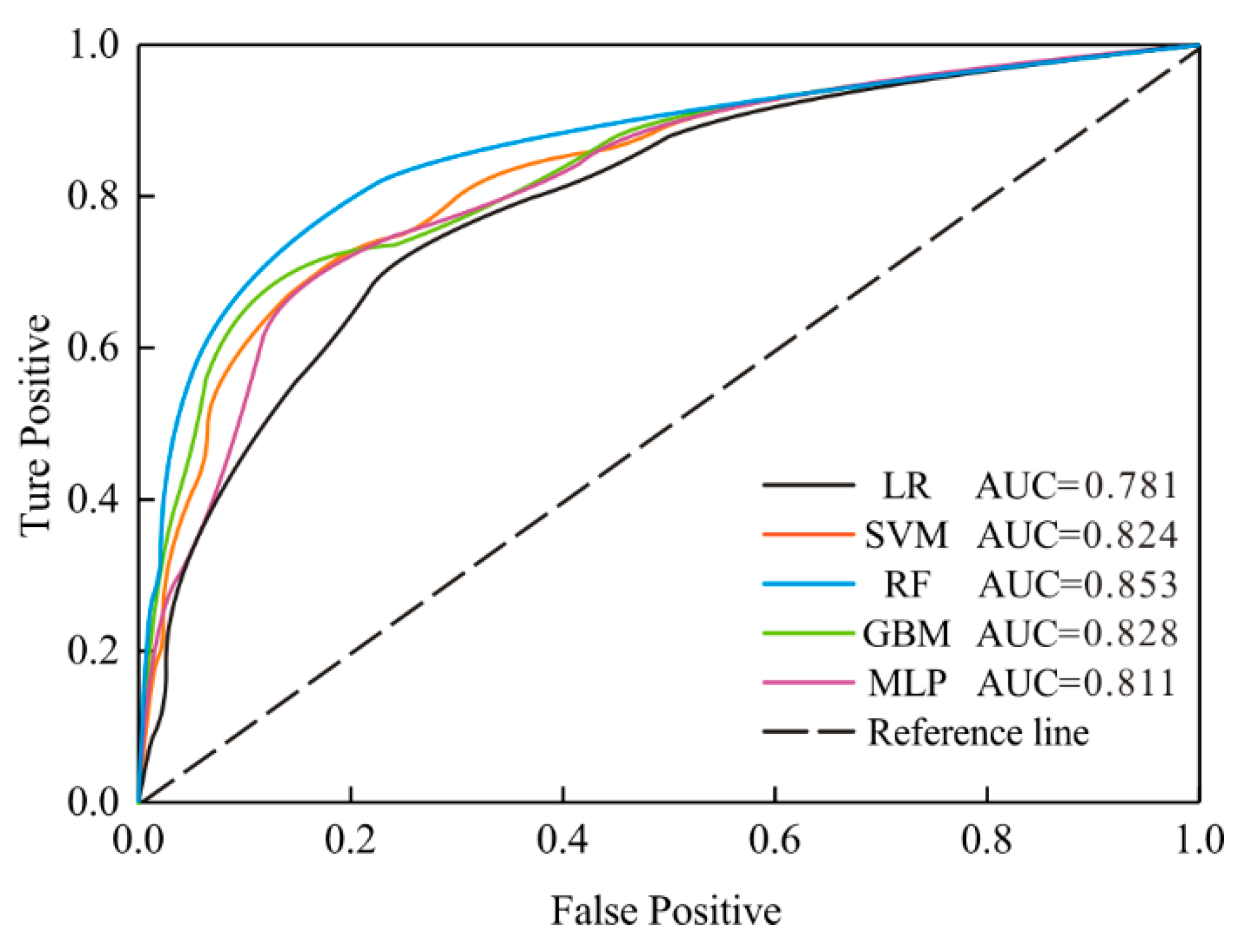
5. Results and Discussion
6. Conclusions
Author Contributions
Funding
Acknowledgments
Conflicts of Interest
References
- Lee, S.; Oh, H.J. Ensemble-Based Landslide Susceptibility Maps in Jinbu Area, Korea. In Terrigenous Mass Movements; Springer: Berlin/Heidelberg, Germany, 2012; pp. 193–220. [Google Scholar]
- Wang, Q.; Li, W.; Wu, Y.; Pei, Y.; Xing, M.; Yang, D. A comparative study on the landslide susceptibility mapping using evidential belief function and weights of evidence models. J. Earth Syst. Sci. 2016, 125, 645–662. [Google Scholar] [CrossRef] [Green Version]
- He, H.; Hu, D.; Sun, Q.; Zhu, L.; Liu, Y. A landslide susceptibility assessment method based on GIS technology and an AHP-weighted information content method: A case study of southern Anhui, China. ISPRS Int. J. Geo-Inf. 2019, 8, 266. [Google Scholar] [CrossRef] [Green Version]
- Liao, Y. Study on Division of Geological Disasters Susceptibility and Meteorological Forecasting and Warning of She County Anhui Province. Ph.D. Thesis, Chengdu University of Technology, Chengdu, China, 2015. [Google Scholar]
- Pan, G. Study on Landslide Distribution, Failure Mechanism and Monitoring in Shexian County of Southern Anhui Province. Ph.D. Thesis, Hefei University of Technology, Hefei, China, 2015. [Google Scholar]
- Banerjee, P.; Ghose, M.K.; Pradhan, R. Analytic hierarchy process and information value method-based landslide susceptibility mapping and vehicle vulnerability assessment along a highway in Sikkim Himalaya. Arab. J. Geosci. 2018, 11, 139. [Google Scholar] [CrossRef]
- El Jazouli, A.; Barakat, A.; Khellouk, R. GIS-multicriteria evaluation using AHP for landslide susceptibility mapping in Oum Er Rbia high basin (Morocco). Geoenviron. Disasters 2019, 6, 3. [Google Scholar] [CrossRef]
- Hepdeniz, K. Using the analytic hierarchy process and frequency ratio methods for landslide susceptibility mapping in Isparta-Antalya highway (D-685), Turkey. Arab. J. Geosci. 2020, 13, 1–16. [Google Scholar] [CrossRef]
- Liu, H.; Li, X.; Meng, T.; Liu, Y. Susceptibility mapping of damming landslide based on slope unit using frequency ratio model. Arab. J. Geosci. 2020, 13, 1–19. [Google Scholar] [CrossRef]
- Senanayake, S.; Pradhan, B.; Huete, A.; Brennan, J. Assessing Soil Erosion Hazards Using Land-Use Change and Landslide Frequency Ratio Method: A Case Study of Sabaragamuwa Province, Sri Lanka. Remote Sens. 2020, 12, 1483. [Google Scholar] [CrossRef]
- Mondal, S.; Mandal, S. Landslide susceptibility mapping of Darjeeling Himalaya, India using index of entropy (IOE) model. Appl. Geomat. 2019, 11, 129–146. [Google Scholar] [CrossRef]
- Shirani, K.; Pasandi, M.; Arabameri, A. Landslide susceptibility assessment by dempster–shafer and index of entropy models, Sarkhoun basin, southwestern Iran. Nat. Hazards 2018, 93, 1379–1418. [Google Scholar] [CrossRef]
- Wang, Q.; Li, W.; Yan, S.; Wu, Y.; Pei, Y. GIS based frequency ratio and index of entropy models to landslide susceptibility mapping (Daguan, China). Environ. Earth Sci. 2016, 75. [Google Scholar] [CrossRef]
- Gadtaula, A.; Dhakal, S. Landslide susceptibility mapping using Weight of Evidence Method in Haku, Rasuwa District, Nepal. J. Nepal Geol. Soc. 2019, 58, 163–171. [Google Scholar] [CrossRef]
- Kumar, R.; Anbalagan, R. Landslide susceptibility mapping of the Tehri reservoir rim area using the weights of evidence method. J. Earth Syst. Sci. 2019, 128, 153. [Google Scholar] [CrossRef] [Green Version]
- Sifa, S.F.; Mahmud, T.; Tarin, M.A.; Haque, D.M.E. Event-based landslide susceptibility mapping using weights of evidence (WoE) and modified frequency ratio (MFR) model: A case study of Rangamati district in Bangladesh. Geol. Ecol. Landsc. 2019, 1–14. [Google Scholar] [CrossRef]
- Chen, X.; Chen, W. GIS-based landslide susceptibility assessment using optimized hybrid machine learning methods. CATENA 2021, 196, 104833. [Google Scholar] [CrossRef]
- Reichenbach, P.; Rossi, M.; Malamud, B.D.; Mihir, M.; Guzzetti, F. A review of statistically-based landslide susceptibility models. Earth-Sci. Rev. 2018, 180, 60–91. [Google Scholar] [CrossRef]
- Regmi, N.R.; Giardino, J.R.; McDonald, E.V.; Vitek, J.D. A comparison of logistic regression-based models of susceptibility to landslides in western Colorado, USA. Landslides 2014, 11, 247–262. [Google Scholar] [CrossRef]
- Shan, Y.; Chen, S.; Zhong, Q. Rapid prediction of landslide dam stability using the logistic regression method. Landslides 2020, 17, 2931–2956. [Google Scholar] [CrossRef]
- Pandey, V.K.; Pourghasemi, H.R.; Sharma, M.C. Landslide susceptibility mapping using maximum entropy and support vector machine models along the Highway Corridor, Garhwal Himalaya. Geocarto Int. 2020, 35, 168–187. [Google Scholar] [CrossRef]
- Pourghasemi, H.R.; Jirandeh, A.G.; Pradhan, B.; Xu, C.; Gokceoglu, C. Landslide susceptibility mapping using support vector machine and GIS at the Golestan Province, Iran. J. Earth Syst. Sci. 2013, 122, 349–369. [Google Scholar] [CrossRef] [Green Version]
- Harmouzi, H.; Nefeslioglu, H.A.; Rouai, M.; Sezer, E.A.; Dekayir, A.; Gokceoglu, C. Landslide susceptibility mapping of the Mediterranean coastal zone of Morocco between Oued Laou and El Jebha using artificial neural networks (ANN). Arab. J. Geosci. 2019, 12, 696. [Google Scholar] [CrossRef]
- Sameen, M.I.; Pradhan, B.; Lee, S. Application of convolutional neural networks featuring Bayesian optimization for landslide susceptibility assessment. Catena 2020, 186, 104249. [Google Scholar] [CrossRef]
- Shahri, A.A.; Spross, J.; Johansson, F.; Larsson, S. Landslide susceptibility hazard map in southwest Sweden using artificial neural network. Catena 2019, 183, 104225. [Google Scholar] [CrossRef]
- Niu, F.; Chen, L. Forecasting of Landslide Stability Based on Gradient Boosting Decision Tree Model. Int. Core J. Eng. 2019, 5, 42–48. [Google Scholar]
- Wu, Y.; Ke, Y.; Chen, Z.; Liang, S.; Zhao, H.; Hong, H. Application of alternating decision tree with AdaBoost and bagging ensembles for landslide susceptibility mapping. Catena 2020, 187, 104396. [Google Scholar] [CrossRef]
- Chen, W.; Fan, L.; Li, C.; Pham, B.T. Spatial prediction of landslides using hybrid integration of artificial intelligence algorithms with frequency ratio and index of entropy in nanzheng county, china. Appl. Sci. 2020, 10, 29. [Google Scholar] [CrossRef] [Green Version]
- Jaafari, A.; Najafi, A.; Pourghasemi, H.; Rezaeian, J.; Sattarian, A. GIS-based frequency ratio and index of entropy models for landslide susceptibility assessment in the Caspian forest, northern Iran. Int. J. Environ. Sci. Technol. 2014, 11, 909–926. [Google Scholar] [CrossRef] [Green Version]
- Li, R.; Wang, N. Landslide susceptibility mapping for the Muchuan county (China): A comparison between bivariate statistical models (woe, ebf, and ioe) and their ensembles with logistic regression. Symmetry 2019, 11, 762. [Google Scholar] [CrossRef] [Green Version]
- Wang, Q.; Li, W.; Chen, W.; Bai, H. GIS-based assessment of landslide susceptibility using certainty factor and index of entropy models for the Qianyang County of Baoji city, China. J. Earth Syst. Sci. 2015, 124, 1399–1415. [Google Scholar] [CrossRef]
- Dikshit, A.; Pradhan, B.; Alamri, A.M. Pathways and challenges of the application of artificial intelligence to geohazards modelling. Gondwana Res. 2020. [Google Scholar] [CrossRef]
- Merghadi, A.; Yunus, A.P.; Dou, J.; Whiteley, J.; ThaiPham, B.; Bui, D.T.; Avtar, R.; Abderrahmane, B. Machine learning methods for landslide susceptibility studies: A comparative overview of algorithm performance. Earth-Sci. Rev. 2020, 207, 103225. [Google Scholar] [CrossRef]
- Yu, X. Study on the Landslide Susceptibility Evaluation Method Based on Multi-Source Data and Multi-Scale Analysis. Ph.D. Thesis, China University, Wuhan, China, 2016. [Google Scholar]
- Bui, D.T.; Ho, T.C.; Pradhan, B.; Pham, B.T.; Nhu, V.H.; Revhaug, I. GIS-based modeling of rainfall-induced landslides using data mining-based functional trees classifier with AdaBoost, Bagging, and MultiBoost ensemble frameworks. Environ. Earth Sci. 2016, 75, 1101. [Google Scholar]
- Feizizadeh, B.; Roodposhti, M.S.; Blaschke, T.; Aryal, J. Comparing GIS-based support vector machine kernel functions for landslide susceptibility mapping. Arab. J. Geosci. 2017, 10, 1–13. [Google Scholar] [CrossRef]
- Van Den Eeckhaut, M.; Vanwalleghem, T.; Poesen, J.; Govers, G.; Verstraeten, G.; Vandekerckhove, L. Prediction of landslide susceptibility using rare events logistic regression: A case-study in the Flemish Ardennes (Belgium). Geomorphology 2006, 76, 392–410. [Google Scholar] [CrossRef]
- Ohlmacher, C.G. Plan curvature and landslide probability in regions dominated by earth flows and earth slides. Eng. Geol. 2007, 91, 117–134. [Google Scholar] [CrossRef]
- Wang, Z.; Hu, Z.; Liu, H.; Gong, H.; Zhao, W.; Yu, M.; Zhang, M. Application of the relief degree of land surface in landslide disasters susceptibility assessment in China. Geoinformatics 2010, 1–5. [Google Scholar] [CrossRef]
- Zhang, J.; Yin, K.; Wang, J.; Liu, L.; Huang, F. Evaluation of landslide susceptibility for Wanzhou district of Three Gorges Reservoir. Chin. J. Rock Mech. Eng. 2016, 35, 284–296. (In Chinese) [Google Scholar]
- Cristinicu, I. Frequency ratio and GIS-based evaluation of landslide susceptibility applied to cultural heritage assessment. J. Cult. Herit. 2017, 28, 172–176. [Google Scholar] [CrossRef]
- Chen, C.-W.; Wei, L.-W.; Lin, G.-W.; Iida, T.; Yamada, R. Evaluating the susceptibility of landslide landforms in Japan using slope stability analysis: A case study of the 2016 Kumamoto earthquake. Landslides 2017, 14, 1793–1801. [Google Scholar] [CrossRef]
- Erener, A.; Mutlu, A.; Duzgun, S. A comparative study for landslide susceptibility mapping using GIS-based multi-criteria decision analysis (MCDA), logistic regression (LR) and association rule mining (ARM). Eng. Geol. 2016, 203, 45–55. [Google Scholar] [CrossRef]
- Dai, C.F.; Lee, F.C.; Li, J.; Xu, W.Z. Assessment of landslide susceptibility on the natural terrain of Lantau Island, Hong Kong. Environ. Earth Sci. 2001, 40, 381–391. [Google Scholar]
- Park, S.; Choi, C.; Kim, B.; Kim, J. Landslide susceptibility mapping using frequency ratio, analytic hierarchy process, logistic regression, and artificial neural network methods at the Inje area, Korea. Environ. Earth Sci. 2012, 68, 1443–1464. [Google Scholar] [CrossRef]
- Yalcin, A. GIS-based landslide susceptibility mapping using analytical hierarchy process and bivariate statistics in Ardesen (Turkey): Comparisons of results and confirmations. Catena 2008, 72, 1–12. [Google Scholar] [CrossRef]
- Gayen, A.; Saha, S.; Pourghasemi, H.R. Soil erosion assessment using RUSLE model and its validation by FR probability model. Geocarto Int. 2020, 35, 1750–1768. [Google Scholar] [CrossRef]
- Moore, D.I.; Grayson, B.R.; Ladson, R.A. Digital terrain modelling: A review of hydrological, geomorphological, and biological applications. Hydrol. Process. 1991, 5, 3–30. [Google Scholar] [CrossRef]
- Mind’je, R.; Li, L.; Nsengiyumva, J.B.; Mupenzi, C.; Nyesheja, E.M.; Kayumba, P.M.; Gasirabo, A.; Hakorimana, E. Landslide susceptibility and influencing factors analysis in Rwanda. Environ. Dev. Sustain. 2019, 22, 7985–8012. [Google Scholar] [CrossRef]
- Tran, Q.C.; Minh, D.D.; Jaafari, A.; Al-Ansari, N.; Minh, D.D.; Van, D.T.; Nguyen, D.A.; Tran, T.H.; Ho, L.S.; Nguyen, D.H.; et al. Novel Ensemble Landslide Predictive Models Based on the Hyperpipes Algorithm: A Case Study in the Nam Dam Commune, Vietnam. Appl. Sci. 2020, 10, 3710. [Google Scholar] [CrossRef]
- Yilmaz, I.; Keskin, I. GIS based statistical and physical approaches to landslide susceptibility mapping (Sebinkarahisar, Turkey). Bull. Eng. Geol. Environ. 2009, 68, 459–471. [Google Scholar] [CrossRef]
- Dong, J.-J.; Tung, Y.-H.; Chen, C.-C.; Liao, J.-J.; Pan, Y.-W. Discriminant analysis of the geomorphic characteristics and stability of landslide dams. Geomorphology 2009, 110, 162–171. [Google Scholar] [CrossRef]
- Gariano, S.L.; Sarkar, R.; Dikshit, A.; Dorji, K.; Brunetti, M.T.; Peruccacci, S.; Melillo, M. Automatic calculation of rainfall thresholds for landslide occurrence in Chukha Dzongkhag, Bhutan. Bull. Eng. Geol. Environ. 2019, 78, 4325–4332. [Google Scholar] [CrossRef]
- Froude, M.J.; Petley, D.N. Global fatal landslide occurrence from 2004 to 2016. Nat. Hazards Earth Syst. Sci. 2018, 18, 2161–2181. [Google Scholar] [CrossRef] [Green Version]
- Dikshit, A.; Sarkar, R.; Pradhan, B.; Segoni, S.; Alamri, A.M. Rainfall Induced Landslide Studies in Indian Himalayan Region: A Critical Review. Appl. Sci. 2020, 10, 2466. [Google Scholar] [CrossRef] [Green Version]
- Dikshit, A.; Sarkar, R.; Pradhan, B.; Acharya, S.; Alamri, A.M. Spatial Landslide Risk Assessment at Phuentsholing, Bhutan. Geosciences 2020, 10, 131. [Google Scholar] [CrossRef] [Green Version]
- Y Bui, T.D.; Bui, T.D.; Nguyen, P.Q.; Hoang, N.-D.; Klempe, H. A novel fuzzy K-nearest neighbor inference model with differential evolution for spatial prediction of rainfall-induced shallow landslides in a tropical hilly area using GIS. Landslides 2017, 14, 1–17. [Google Scholar]
- Xianyu, Y.; Yi, W.; Ruiqing, N.; Youjian, H. A Combination of Geographically Weighted Regression, Particle Swarm Optimization and Support Vector Machine for Landslide Susceptibility Mapping: A Case Study at Wanzhou in the Three Gorges Area, China. Int. J. Environ. Res. Public Health 2016, 13, 487. [Google Scholar] [CrossRef] [Green Version]
- Das, G.; Lepcha, K. Application of logistic regression (LR) and frequency ratio (FR) models for landslide susceptibility mapping in Relli Khola river basin of Darjeeling Himalaya, India. SN Appl. Sci. 2019, 1, 1453. [Google Scholar] [CrossRef] [Green Version]
- Hosmer, W.D.; Stanley, L. Applied logistic regression. Contemp. Sociol. 2000. [Google Scholar] [CrossRef]
- Battiti, R.; Brunato, M. Machine Learning Plus Intelligent Optimization; Lionsolver Inc.: Los Angeles, CA, USA, 2013. [Google Scholar]
- Lee, S.; Lee, M.-J.; Lee, S. Spatial prediction of urban landslide susceptibility based on topographic factors using boosted trees. Environ. Earth Sci. 2018, 77, 656. [Google Scholar] [CrossRef]
- Wang, Y.; Sun, D.; Wen, H.; Zhang, H.; Zhang, F. Comparison of Random Forest Model and Frequency Ratio Model for Landslide Susceptibility Mapping (LSM) in Yunyang County (Chongqing, China). Int. J. Environ. Res. Public Health 2020, 17, 4206. [Google Scholar] [CrossRef]
- Breiman, L. Random Forests. Mach. Learn. 2001, 45, 5–32. [Google Scholar] [CrossRef] [Green Version]
- Ho, T.K. The random subspace method for constructing decision forests. IEEE Trans. Pattern Anal. Mach. Intell. 1998, 20, 832–844. [Google Scholar]
- Sahin, K.E. Assessing the predictive capability of ensemble tree methods for landslide susceptibility mapping using XGBoost, gradient boosting machine, and random forest. SN Appl. Sci. 2020, 2, 1–17. [Google Scholar] [CrossRef]
- Pham, B.T.; Tien Bui, D.; Pourghasemi, H.R.; Indra, P.; Dholakia, M.B. Landslide susceptibility assesssment in the Uttarakhand area (India) using GIS: A comparison study of prediction capability of nave bayes, multilayer perceptron neural networks, and functional trees methods. Theor. Appl. Climatol. 2015, 122, 1–19. [Google Scholar] [CrossRef]
- Zare, M.; Pourghasemi, H.R.; Vafakhah, M.; Pradhan, B. Landslide susceptibility mapping at Vaz Watershed (Iran) using an artificial neural network model: A comparison between multilayer perceptron (MLP) and radial basic function (RBF) algorithms. Arab. J. Geosci. 2013, 6, 2873–2888. [Google Scholar] [CrossRef]
- Hornik, K.; Stinchcombe, M.; White, H. Multilayer feedforward networks are universal approximators. Neural Netw. 1989, 2, 359–366. [Google Scholar] [CrossRef]
- Chen, J.; Yang, S.; Li, H.; Zhang, B.; Lv, J. Research on geographical environment unit division based on the method of natural breaks (Jenks). Int. Arch. Photogramm. Remote Sens. Spat. Inf. Sci. 2013, 3, 47–50. [Google Scholar] [CrossRef] [Green Version]
- Hanley, A.J.; McNeil, J.B. The meaning and use of the area under a receiver operating characteristic (ROC) curve. Radiology 1982, 143, 29–36. [Google Scholar] [CrossRef] [Green Version]
- Fawcett, T. An introduction to ROC analysis. Pattern Recognit. Lett. 2005, 27, 861–874. [Google Scholar] [CrossRef]


| Group | Stratum and Lithology |
|---|---|
| 1 | Mesoproterozoic. Black slate with light metamorphic lithic arkose and siltstone. |
| 2 | Lower Sinian. This is composed of grayish green and purplish red argillaceous conglomerate, gravelly sandstone and gravelly sandstone with a small amount of mudstone. |
| 3 | Middle Sinian. Gray black, light gray, thin-thick layer siliceous rock and siliceous shale. |
| 4 | Cambrian. Argillaceous limestone and dolomitic limestone are mainly mixed with a thin marl, carbonaceous and calcareous mudstone. |
| 5 | Quaternary. Pebble sandy fine gravel layer, silty sand clay layer, gravel, sandy soil layer and gravelly loam. |
| 6 | Granite |
Publisher’s Note: MDPI stays neutral with regard to jurisdictional claims in published maps and institutional affiliations. |
© 2020 by the authors. Licensee MDPI, Basel, Switzerland. This article is an open access article distributed under the terms and conditions of the Creative Commons Attribution (CC BY) license (http://creativecommons.org/licenses/by/4.0/).
Share and Cite
Wang, Z.; Liu, Q.; Liu, Y. Mapping Landslide Susceptibility Using Machine Learning Algorithms and GIS: A Case Study in Shexian County, Anhui Province, China. Symmetry 2020, 12, 1954. https://doi.org/10.3390/sym12121954
Wang Z, Liu Q, Liu Y. Mapping Landslide Susceptibility Using Machine Learning Algorithms and GIS: A Case Study in Shexian County, Anhui Province, China. Symmetry. 2020; 12(12):1954. https://doi.org/10.3390/sym12121954
Chicago/Turabian StyleWang, Zitao, Qimeng Liu, and Yu Liu. 2020. "Mapping Landslide Susceptibility Using Machine Learning Algorithms and GIS: A Case Study in Shexian County, Anhui Province, China" Symmetry 12, no. 12: 1954. https://doi.org/10.3390/sym12121954
APA StyleWang, Z., Liu, Q., & Liu, Y. (2020). Mapping Landslide Susceptibility Using Machine Learning Algorithms and GIS: A Case Study in Shexian County, Anhui Province, China. Symmetry, 12(12), 1954. https://doi.org/10.3390/sym12121954