A Parametric Quantile Regression Model for Asymmetric Response Variables on the Real Line

Abstract

In this paper, we introduce a novel parametric quantile regression model for asymmetric response variables, where the response variable follows a power skew-normal distribution. By considering a new convenient parametrization, these distribution results are very useful for modeling different quantiles of a response variable on the real line. The maximum likelihood method is employed to estimate the model parameters. Besides, we present a local influence study under different perturbation settings. Some numerical results of the estimators in finite samples are illustrated. In order to illustrate the potential for practice of our model, we apply it to a real dataset.

1. Introduction

Frequently, in real life, we find continuous data on the real line that are asymmetrical; these data cannot be modeled by known symmetric distributions as the normal, Student-t, Cauchy, Laplace, and logistic distributions. It is therefore more interesting to propose more flexible models that will be useful for modeling highly skewed data which arises in several areas.

In this context, the seminal work in Azzalini [1] introduces a skew-symmetric family of distributions, where this last is established by using a symmetric distribution as a kernel. When this last follows a normal distribution, it rises the well-know skew-normal (SN) distribution. The SN distribution has a skewness parameter which makes possible to have a reasonable model for a skewed distribution. Furthermore, the SN distributions include the normal distribution and possesses several properties which coincide or are similar to the ones of the normal distribution (Azzalini [1,2]). However, the SN distribution is limited in terms of flexibility, that is, for moderate values of the skewness parameter nearly all the mass accumulates either on the positive or negative real line, as determined by the sign of the skewness parameter. In such cases, the SN distribution closely resembles the half-normal density, with a nearly linear shape in the side with smaller mass (Arellano-Valle et al. [3]).

Another alternative to model skewed data is using the family of power-symmetric distributions (see Pewsey et al. [4]) of which the most widely used is the power-normal (PN) distribution. Some references where this family is discussed are Lehmann [5], Durrans [6], Gupta and Gupta [7], Castillo et al. [8], among others. In a series of papers by Martínez-Flórez et al. ([9,10,11,12,13]) extensions and applications of the PN distribution can be found.

An unification of the SN and PN distributions was proposed by Martínez-Flórez et al. [11], namely the power skew-normal (PSN) which is a generalization of the SN and PN distributions. Even though sample information about the SN distribution has been widely studied, there is not the same scope for the PSN distribution, which being a generalization of the first one, has characteristics of interest such as: (i) the SN and PN distributions as particular cases, and (ii) the PSN distribution provides greater range for skewness and kurtosis coefficients compared with the SN distribution (see Table 1), being more flexible to model highly skewed data, which arises frequently in many practical situations. However, the expectation and variance of the PSN distribution cannot be expressed in closed form (have complicated forms), which makes these distributions unsuitable for regression modeling (Martínez-Flórez et al. [11]). Fortunately, the cumulative distribution function (cdf) of the PSN distribution has a simple form that depends on Owen’s T function (to be defined in the next section). This facilitates the calculation of the quantile function (inverse of the cdf), allowing its utilization in the quantile regression (QR) framework. Quantile regression quantifies the association of the explanatory variables with a given quantile of a dependent variable. In this study, we propose a quantile linear regression model based on the PSN distribution, adopting a new parametrization of this model indexed by the quantile, precision and shape parameters. In particular, for this work, inference is conducted via maximum likelihood.

Table 1. Range for skewness and kurtosis coefficients for SN, PN and PSN models.

Coefficient	SN	PN	PSN
Skewness	(−0.9953, 0.9953)	[−0.6115, 0.9007]	[−1.6476, 0.9953)
Kurtosis	[3, 3.8692)	[1.7170, 4.3556]	[1.4672, 5.4386]

The rest of the paper proceeds as follows. In Section 2, we introduce a new parameterization of the PSN distribution that is indexed by the location, precision and shape parameters and its association with a quantile regression model. In addition, elements related to the maximum likelihood (ML) method are presented as well. Section 3 presents local influence measures under three different perturbation schemes, whereas in Section 4 a real data analysis is conducted in order to show the applicability of our proposed reparametrized PSN (RPSN) based QR model. Final section summarizes the contributions of the paper.

2. A PSN Distribution Parameterized by Its Quantile Parameter, and Its Associated Quantile Regression Model

In this section, we briefly study the PSN distribution based on Martínez-Flórez et al. [11]. We introduce a RPSN distribution which is characterized by its quantile, which allows us to use this distribution in the context of QR models.

The probability density function (pdf) of the PSN distribution is given by

$$\begin{array}{c}\hfill f(y;\mathbf{\theta })=\frac{\alpha }{\sigma }{\varphi }_{\lambda }\left(z\right){\left[{\mathsf{\Phi }}_{\lambda }\left(z\right)\right]}^{\alpha -1},\end{array}$$

where $\mathbf{\theta }={(\mu ,\sigma ,\lambda ,\alpha )}^{\top }$, $z=(y-\mu )/\sigma$ and ${\varphi }_{\lambda }(·)$ and ${\mathsf{\Phi }}_{\lambda }(·)$ denote the pdf and cdf of the (standard) skew normal model given by

$${\varphi }_{\lambda }\left(y\right)=2\varphi \left(y\right)\mathsf{\Phi }\left(\lambda y\right)\mathrm{and}{\mathsf{\Phi }}_{\lambda }\left(y\right)={\int }_{-\infty }^y{\varphi }_{\lambda }\left(t\right)\mathrm{d}t=\mathsf{\Phi }\left(y\right)-2T(y,\lambda ),$$

where $\varphi (·)$ and $\mathsf{\Phi }(·)$ denote the pdf and cdf of the standard normal distribution and $T(·,·)$ is the Owen’s T function defined as

$$T(y,\lambda )=\frac{1}{2\pi }{\int }_0^{\lambda }\frac{{\mathrm{e}}^{-\frac{1}{2}{y}^2(1+t^2)}}{1+t^2}\mathrm{d}t.$$

Moreover, the cdf of the PSN model is given by

$$\begin{array}{c}\hfill F(y;\mathbf{\theta })={\left[{\mathsf{\Phi }}_{\lambda }\left(z\right)\right]}^{\alpha }={\left[\mathsf{\Phi }\left(z\right)-2T\left(z,\lambda \right)\right]}^{\alpha }.\end{array}$$

Note that $\alpha =1$ and $\lambda =0$ corresponds to the very well known SN and PN models, respectively. The main advantage of the PSN model is that provides greater range for skewness and kurtosis coefficients compared with the SN and PN models. Table 1 shows the range for those coefficients.

The r-th moment of the distribution depends on the expected value of ${\left[{\mathsf{\Phi }}_{\lambda }^{-1}\left(Y\right)\right]}^s$, $s=1,\dots ,r$, where Y have beta distribution with shape parameters $\alpha$ and 1, respectively. For this reason, some interesting characteristic of the model, such as mean and variance, have cumbersome forms. On the other hand, quantiles of the model also need to be computed numerically since non-closed form are available for the distribution. For this reason, non-interpretation and useful reparametrizations can be performed for this model. Besides, as the Owen’s T function satisfies $T(0,\lambda )={\left(2\pi \right)}^{-1}arctan\left(\lambda \right)$, we note that

$$\begin{array}{c}\hfill F(\mu ;\mathbf{\theta })={\left[\frac{1}{2}-\frac{1}{\pi }arctan\left(\lambda \right)\right]}^{\alpha }.\end{array}$$

For this reason, if we consider the restriction

$$\begin{array}{c}\hfill \alpha =\alpha (\lambda ,\tau )=\frac{log\left(\tau \right)}{log\left(\frac{1}{2}-\frac{1}{\pi }arctan\left(\lambda \right)\right)},\end{array}$$

(1)

we have that $F(\mu ;\mathbf{\theta })=\tau$ with $\mu$ representing directly the $\tau$-th quantile of the distribution. For a fixed $\tau$ and considering $\alpha (\lambda ,\tau )$ as in (1), we have a flexible model for quantile regression. This parametrization has not been proposed in the statistical literature. Hence, we can rewrite the PSN distribution according to the parameters $\mu ,\sigma$ and $\lambda$, whose cumulative distribution function is now given by

$$\begin{array}{c}\hfill F(y;\mu ,\sigma ,\lambda )={\left[\mathsf{\Phi }\left(z\right)-2T\left(z,\lambda \right)\right]}^{\frac{log\left(\tau \right)}{log\left(\frac{1}{2}-\frac{1}{\pi }arctan\left(\lambda \right)\right)}},\end{array}$$

where the quantile $\tau \in (0,1)$ is assumed to be known. Hereafter, we use the notation $Y\sim \mathrm{RPSN}(\mu ,\sigma ,\lambda )$ to indicate that Y is a random variable following a restricted PSN distribution with quantile parameter $\mu$, precision parameter $\sigma$, and shape parameter $\lambda$. Figure 1 shows the density function for the RPSN model with location and scale parameters fixed at 0 and 1, respectively. Note that in all the curves, the zero represents the specified quantile $\tau$. We also note that the curves are not necessarily symmetric for $\tau =0.5$ (the median case).

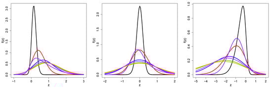
Figure 1. Pdf for the RPSN$(\mu =0,\sigma =1,\lambda )$ for different values of $\lambda$: $\tau =0.1$ (left panel); $\tau =0.5$ (center panel); $\tau =0.9$ (right panel). Values for $\lambda$ are: $-5$ (black line), $-1.5$ (red line), $-0.5$ (blue line), 0 (green line), $0.5$ (orange line), $1.5$ (magenta line) and 5 (purple line).

Let $Y_1,\dots ,Y_n$ be the n independent random variables, where each $Y_i,i=1,\dots ,n$, follows the $\mathrm{PSN}$ distribution with quantile parameter $\mu$, precision parameter $\sigma$, and shape parameter $\lambda$. Suppose that, for a given $\tau \in (0,1)$, the location, precision and shape parameters for the RPSN satisfy the following functional relations

$$\begin{array}{cc}\hfill g_1\left({\mu }_i\left(\tau \right)\right)& ={\eta }_{i1}\left(\tau \right)={\mathbf{x}}_{i1}^{\top }{\mathbf{\beta }}_1\left(\tau \right),\hfill \\ \hfill g_2\left({\sigma }_i\left(\tau \right)\right)& ={\eta }_{i2}\left(\tau \right)={\mathbf{x}}_{i2}^{\top }{\mathbf{\beta }}_2\left(\tau \right)\mathrm{and}\hfill \\ \hfill g_3\left({\lambda }_i\left(\tau \right)\right)& ={\eta }_{i3}\left(\tau \right)={\mathbf{x}}_{i3}^{\top }{\mathbf{\beta }}_3\left(\tau \right),\hfill \end{array}$$

(2)

where ${\mathbf{\beta }}_j\left(\tau \right)={({\beta }_{j1}\left(\tau \right),\dots ,{\beta }_{j{p}_1}\left(\tau \right))}^{\top }$, $j=1,2,3$, are vectors of unknown regression coefficients which are assumed to be functionally independent, ${\mathbf{\beta }}_j\left(\tau \right)\in {\mathbb{R}}^{p_j}$, with $p_1+p_2+p_3<n$, ${\eta }_{ji}\left(\tau \right)$ are the linear predictors, and ${\mathbf{x}}_{ij}={(x_{ij1},\dots ,x_{ij{p}_j})}^{\top }$, are observations on $p_1$, $p_2$ and $p_3$ known regressors, for $i=1,\dots ,n$. Moreover covariate matrices ${\mathbf{X}}_j={({\mathbf{x}}_{1j},\dots ,{\mathbf{x}}_{nj})}^{\top }$ are assumed to have rank $p_j$, for $j=1,2,3$. Link functions $g_1:\mathbb{R}\to \mathbb{R}$, $g_2:\mathbb{R}\to {\mathbb{R}}^{+}$ and $g_3:\mathbb{R}\to \mathbb{R}$ in (2) must be strictly monotone and at least twice differentiable, and $g_2$ is also required to be a positive function. Such functions also satisfy that ${\mu }_i=g_1^{-1}\left({\mathbf{x}}_{i1}^{\top }{\mathbf{\beta }}_1\right)$, ${\sigma }_i=g_2^{-1}\left({\mathbf{x}}_{i2}^{\top }{\mathbf{\beta }}_2\right)$ and ${\lambda }_i=g_3^{-1}\left({\mathbf{x}}_{i3}^{\top }{\mathbf{\beta }}_3\right)$, with $g_j^{-1}(·)$ being the inverse function of $g_j(·)$.

The log-likelihood function for $\mathbf{\theta }=\mathbf{\theta }\left(\tau \right)=({\mathbf{\beta }}_1\left(\tau \right),{\mathbf{\beta }}_2\left(\tau \right),{\mathbf{\beta }}_3\left(\tau \right))$ has the form $\ell \left(\mathbf{\theta }\right)={\sum }_{i=1}^n{\ell }_i$, where

$$\begin{array}{ccc}\hfill {\ell }_i=\ell (z_i,{\mu }_i,{\sigma }_i,{\lambda }_i)& =& log\alpha ({\lambda }_i,\tau )-log\left({\sigma }_i\right)+log\left[{\varphi }_{{\lambda }_i}\left(z_i\right)\right]+\left[\alpha ({\lambda }_i,\tau )-1\right]log\left[{\mathsf{\Phi }}_{{\lambda }_i}\left(z_i\right)\right].\hfill \end{array}$$

(3)

The $(p_1+p_2+p_3)\times 1$ score vector of the model is given by

$$\begin{array}{c}\hfill \dot{\ell }\left(\mathbf{\theta }\right)=\left(\begin{array}{c}\frac{\partial \ell \left(\mathbf{\theta }\right)}{\partial {\mathbf{\beta }}_1}\\ \frac{\partial \ell \left(\mathbf{\theta }\right)}{\partial {\mathbf{\beta }}_2}\\ \frac{\partial \ell \left(\mathbf{\theta }\right)}{\partial {\mathbf{\beta }}_3}\end{array}\right)=\left(\begin{array}{c}{\mathbf{X}}_1^{\top }{\mathbf{W}}_{{\mathbf{\beta }}_1}^{1/2}{\dot{\ell }}_{\mu }\\ {\mathbf{X}}_2^{\top }{\mathbf{W}}_{{\mathbf{\beta }}_2}^{1/2}{\dot{\ell }}_{\sigma }\\ {\mathbf{X}}_3^{\top }{\mathbf{W}}_{{\mathbf{\beta }}_3}^{1/2}{\dot{\ell }}_{\lambda }\end{array}\right),\end{array}$$

(4)

where ${\mathbf{W}}_{{\mathbf{\beta }}_j}=\mathrm{diag}(w_{{\beta }_{j1}},\dots ,w_{{\beta }_{jn}})$, $w_{{\beta }_{1i}}={(\partial {\mu }_i/\partial {\eta }_{1i})}^2$, $w_{{\beta }_{2i}}={(\partial {\sigma }_i/\partial {\eta }_{2i})}^2$, $w_{{\beta }_{3i}}={(\partial {\lambda }_i/\partial {\eta }_{3i})}^2$, ${\dot{\ell }}_{\xi }=({\dot{\ell }}_{{\xi }_1},\dots ,{\dot{\ell }}_{{\xi }_n})$, for $\xi \in \{\mu ,\sigma ,\lambda \}$, with ${\dot{\ell }}_{{\xi }_i}=\partial \ell ({\mu }_i,{\sigma }_i,{\lambda }_i)/\partial {\xi }_i$. Such elements are specified in the Appendix A.1 Section.

The Hessian for the model is

$$\begin{array}{cc}\hfill \mathit{H}(\mathbf{\theta })& =\left(\begin{array}{ccc}{\mathit{H}}_{{\mathbf{\beta }}_1{\mathbf{\beta }}_1}& {\mathit{H}}_{{\mathbf{\beta }}_1{\mathbf{\beta }}_2}& {\mathit{H}}_{{\mathbf{\beta }}_1{\mathbf{\beta }}_3}\\ ·& {\mathit{H}}_{{\mathbf{\beta }}_2{\mathbf{\beta }}_2}& {\mathit{H}}_{{\mathbf{\beta }}_2{\mathbf{\beta }}_3}\\ ·& ·& {\mathit{H}}_{{\mathbf{\beta }}_3{\mathbf{\beta }}_3}\end{array}\right)\hfill \\ \hfill & =\left(\begin{array}{ccc}{\mathbf{X}}_1^{\top }{\ddot{\ell }}_{\mathbf{\mu }\mathbf{\mu }}{\mathbf{W}}_{{\mathbf{\beta }}_1}{\mathbf{X}}_1& {\mathbf{X}}_1^{\top }{\ddot{\ell }}_{\mathbf{\mu }\mathbf{\sigma }}{\mathbf{W}}_{{\mathbf{\beta }}_1}^{1/2}{\mathbf{W}}_{{\mathbf{\beta }}_2}^{1/2}{\mathbf{X}}_2& {\mathbf{X}}_1^{\top }{\ddot{\ell }}_{\mathbf{\mu }\mathbf{\lambda }}{\mathbf{W}}_{{\mathbf{\beta }}_1}^{1/2}{\mathbf{W}}_{{\mathbf{\beta }}_3}^{1/2}{\mathbf{X}}_3\\ ·& {\mathbf{X}}_2^{\top }{\ddot{\ell }}_{\mathbf{\sigma }\mathbf{\sigma }}{\mathbf{W}}_{{\mathbf{\beta }}_2}{\mathbf{X}}_2& {\mathbf{X}}_2^{\top }{\ddot{\ell }}_{\mathbf{\sigma }\mathbf{\lambda }}{\mathbf{W}}_{{\mathbf{\beta }}_2}^{1/2}{\mathbf{W}}_{{\mathbf{\beta }}_3}^{1/2}{\mathbf{X}}_3\\ ·& ·& {\mathbf{X}}_3^{\top }{\ddot{\ell }}_{\mathbf{\lambda }\mathbf{\lambda }}{\mathbf{W}}_{{\mathbf{\beta }}_3}{\mathbf{X}}_3\end{array}\right),\hfill \end{array}$$

(5)

where ${\ddot{\ell }}_{\mathbf{\xi }{\mathbf{\xi }}^{{}^{\prime }}}=\mathrm{diag}({\ddot{\ell }}_{{\xi }_1{\xi }_1^{{}^{\prime }}},\dots ,{\ddot{\ell }}_{{\xi }_n{\xi }_n^{{}^{\prime }}})$, for $\xi ,{\xi }^{{}^{\prime }}\in \{\mu ,\sigma ,\lambda \}$, with ${\dot{\ell }}_{{\xi }_i{\xi }_i^{{}^{\prime }}}={\partial }^2{\ell }_i/\partial {\xi }_i\partial {\xi }_i^{{}^{\prime }}$. Such elements are detailed in the Appendix A.1.

The ML estimators ${\widehat{\mathbf{\beta }}}_1\left(\tau \right)$, ${\widehat{\mathbf{\beta }}}_2\left(\tau \right)$ and ${\widehat{\mathbf{\beta }}}_3\left(\tau \right)$ of ${\mathbf{\beta }}_1\left(\tau \right)$, ${\mathbf{\beta }}_2\left(\tau \right)$ and ${\mathbf{\beta }}_3\left(\tau \right)$, respectively, can be obtained by solving simultaneously the nonlinear system of equations $\ell \left(\mathbf{\theta }\right)={\mathbf{0}}_{p_1+p_2+p_3}$, where ${\mathbf{0}}_r$ denotes a vector of zeros with dimension r. Unfortunately, it is not possible to obtain analytical expressions for the ML estimators above, so numerical methods for solving nonlinear equations system are required.

3. Local Influence

Global influence is related to case deletion, i.e, the effect of dropping a case from the dataset Cook [14]. The likelihood distance (LD) is defined as LD$\left(\mathbf{\omega }\right)=2[\ell \left(\widehat{\mathbf{\theta }}\right)-\ell (\widehat{\mathbf{\theta }}\left(\mathbf{\omega }\right),\mathbf{\omega })]$, where $\widehat{\mathbf{\theta }}\left(\mathbf{\omega }\right)$ is the ML estimate of $\mathbf{\theta }$ under a perturbed model related to $\mathbf{\omega }={({\omega }_1,\dots ,{\omega }_n)}^{\top }$, a perturbation vector. Cook [14] studied the LD$\left(\mathbf{\omega }\right)$ around the non-perturbed vector ${\mathbf{\omega }}_0$ such as $\widehat{\mathbf{\theta }}\left({\mathbf{\omega }}_0\right)=\widehat{\mathbf{\theta }}$. The normal curvature for $\widehat{\mathbf{\omega }}$ at the direction of the orthonormal vector $\left|\right|\mathit{d}\left|\right|$ is defined as $C_{\mathit{d}}\left(\widehat{\mathbf{\theta }}\right)=2\left|{\mathit{d}}^{\top }{\mathsf{\Delta }}_{\mathbf{\omega }}^{\top }{\ddot{\ell }}_{\widehat{\mathbf{\theta }}\widehat{\mathbf{\theta }}}{\mathsf{\Delta }}_{\mathbf{\omega }}\mathit{d}\right|$, where ${\ddot{\ell }}_{\widehat{\mathbf{\theta }}\widehat{\mathbf{\theta }}}$ is the Hessian of $\ell \left(\mathbf{\theta }\right)$ evaluated at $\mathbf{\theta }=\widehat{\mathbf{\theta }}$ and ${\mathsf{\Delta }}_{\mathbf{\omega }}={\partial }^2\ell (\mathbf{\theta },\mathbf{\omega })/\partial \mathbf{\theta }\partial {\mathbf{\omega }}^{\top }{\mid }_{\mathbf{\theta }=\widehat{\mathbf{\theta }}\left(\mathbf{\omega }\right)}$ and both, ${\mathsf{\Delta }}_{\mathbf{\omega }}$ and ${\ddot{\ell }}_{\widehat{\mathbf{\theta }}\widehat{\mathbf{\theta }}}$ are evaluated at $\widehat{\mathbf{\theta }}\left(\mathbf{\omega }\right)$. Hence, $C_{d_{\mathtt{max}}}$ is the largest eigenvalue of $\mathbf{B}={\mathsf{\Delta }}_{{\mathbf{\omega }}_0}^{\top }{\ddot{\ell }}_{\widehat{\mathbf{\theta }}\widehat{\mathbf{\theta }}}{\mathsf{\Delta }}_{{\mathbf{\omega }}_0}$ and ${\mathit{d}}_{\mathtt{max}}$ the corresponding orthonormal eigenvector. The index $d_{\mathtt{max}}$ plot of the matrix $\mathbf{B}$ suggests how to perturb the model (or data) to obtain large changes in the estimates of $\mathbf{\theta }$.

For three common perturbation schemes we compute the matrix

$${\mathsf{\Delta }}_{\mathbf{\omega }}=\frac{{\partial }^2\ell (\mathbf{\theta },\mathbf{\omega })}{\partial \mathbf{\theta }\partial \mathbf{\omega }}={\left(\begin{array}{ccc}{\mathsf{\Delta }}_{\mathbf{\omega },{\mathbf{\beta }}_1}^{\top }& {\mathsf{\Delta }}_{\mathbf{\omega },{\mathbf{\beta }}_2}^{\top }& {\mathsf{\Delta }}_{\mathbf{\omega },{\mathbf{\beta }}_3}^{\top }\end{array}\right)}^{\top },$$

where ${\mathsf{\Delta }}_{\mathbf{\omega },{\mathbf{\beta }}_j}^{\top }=\frac{{\partial }^2\ell (\mathbf{\theta },\mathbf{\omega })}{\partial {\mathbf{\beta }}_1\partial \mathbf{\omega }}$.

3.1. Case Weights Perturbation

For this case, the perturbed log-likelihood function is defined as $\ell (\mathbf{\theta },\mathbf{\omega })={\sum }_{i=1}^n{\omega }_i{\ell }_i$, where $\ell (z_i,{\mu }_i,{\sigma }_i,{\lambda }_i)$ is defined in (3) and $0\le {\omega }_i\le 1$, for $i=1,\dots ,n$. In this case, ${\mathbf{\omega }}_0=(1,\dots ,1)$ and

$${\mathsf{\Delta }}_{\mathbf{\omega }}={\left(\begin{array}{ccc}{\mathbf{X}}_1^{\top }{\mathbf{W}}_{{\mathbf{\beta }}_1}^{1/2}{\dot{\ell }}_{\mathbf{\mu }}^{\top }& {\mathbf{X}}_2^{\top }{\mathbf{W}}_{{\mathbf{\beta }}_2}^{1/2}{\dot{\ell }}_{\mathbf{\sigma }}^{\top }& {\mathbf{X}}_3^{\top }{\mathbf{W}}_{{\mathbf{\beta }}_3}^{1/2}{\dot{\ell }}_{\mathbf{\lambda }}^{\top }\end{array}\right)}^{\top }.$$

3.2. Case Response Perturbation

We consider now an additive perturbation on the ith response (say $y_i(·))$ by making $y_i\left({\omega }_i\right)=y_i+{\omega }_i{S}_{Y_i}$, where ${\omega }_i\in \mathbb{R}$ and $S_{Y_i}$ is a scale factor. An usual consideration for such scale factor is $S_{Y_i}=S_Y$, with $S_Y$ denoting the sample standard deviation of Y. Note that ${\mathbf{\omega }}_0=(0,\dots ,0)$. Therefore, under the scheme of response perturbation, the log-likelihood function is given by $\ell (\mathbf{\theta },\mathbf{\omega })={\sum }_{i=1}^n\ell (z_i\left({\omega }_i\right),{\mu }_i,{\sigma }_i,{\lambda }_i)$, where $z_i\left({\omega }_i\right)=(y_i\left({\omega }_i\right)-{\mu }_i)/{\sigma }_i$ and

$${\mathsf{\Delta }}_{\mathbf{\omega }}=S_Y{\left(\begin{array}{ccc}{\mathbf{X}}_1^{\top }{\mathbf{W}}_{{\mathbf{\beta }}_1}^{1/2}{\ddot{\ell }}_{\mathbf{\mu }\mathbf{\mu }}^{\top }& {\mathbf{X}}_2^{\top }{\mathbf{W}}_{{\mathbf{\beta }}_2}^{1/2}{\ddot{\ell }}_{\mathbf{\mu }\mathbf{\sigma }}^{\top }& {\mathbf{X}}_3^{\top }{\mathbf{W}}_{{\mathbf{\beta }}_3}^{1/2}{\ddot{\ell }}_{\mathbf{\mu }\mathbf{\lambda }}^{\top }\end{array}\right)}^{\top }{|}_{{}_{z_i=z_i\left({\omega }_i\right)}}.$$

3.3. Case Continuous Covariate Perturbation

Consider an additive perturbation on a particular continuous covariate including on the quantile parameter, namely $x_t$, for $t\in \{1,\dots ,p_1\}$, by making $x_{it}\left({\omega }_i\right)=x_{it}+{\omega }_i{S}_{X_{it}}$, where $S_{X_{it}}$ is a scale factor. Again, a usual consideration is $S_{X_{it}}=S_{X_t}$, with $S_{X_t}$ the sample standard deviation for $X_t$. Note that ${\mathbf{\omega }}_0=(0,\dots ,0)$. Then, under the scheme of response perturbation, the log-likelihood function is given by $\ell (\mathbf{\theta },\mathbf{\omega })={\sum }_{i=1}^n\ell (z_i,{\mu }_i\left({\omega }_i\right),{\sigma }_i,{\lambda }_i)$, where ${\mu }_i\left({\omega }_i\right)=g_1^{-1}\left({\mathbf{x}}_{i1}^{\top }\left({\omega }_i\right){\mathbf{\beta }}_1\right)$ and ${\mathbf{x}}_{i1}^{\top }\left({\omega }_i\right)={\mathbf{x}}_{i1}^{\top }+{\omega }_i{S}_{X_{it}}{\mathcal{J}}_t$, with ${\mathcal{J}}_t$ a vector of dimension $p_1$ with zeros, except in the t-th element where is a one. Finally

$${\mathsf{\Delta }}_{\mathbf{\omega }}=S_{X_t}{\left(\begin{array}{ccc}\mathrm{diag}\left({\mathcal{J}}_t\right){\mathbf{X}}_1^{\top }{\mathbf{W}}_{{\mathbf{\beta }}_1}^{1/2}{\ddot{\ell }}_{\mathbf{\mu }\mathbf{\mu }}^{\top }& \mathrm{diag}\left({\mathcal{J}}_t\right){\mathbf{X}}_2^{\top }{\mathbf{W}}_{{\mathbf{\beta }}_2}^{1/2}{\ddot{\ell }}_{\mathbf{\mu }\mathbf{\sigma }}^{\top }& \mathrm{diag}\left({\mathcal{J}}_t\right){\mathbf{X}}_3^{\top }{\mathbf{W}}_{{\mathbf{\beta }}_3}^{1/2}{\ddot{\ell }}_{\mathbf{\mu }\mathbf{\lambda }}^{\top }\end{array}\right)}^{\top }{|}_{{}_{z_i=z_i\left({\omega }_i\right)}}.$$

4. Real Data Analysis

In this section, we present an application to 202 Australian athletes from the Australian Institute of Sport. Such data were discussed in Cook and Weisberg [15]. In order to exemplify the proposed model, we consider the following quantile regression model: ${\mathtt{bmi}}_i\left(\tau \right)={\mu }_i\left(\tau \right)+{\sigma }_i\left(\tau \right){ϵ}_i\left(\tau \right)$, where ${ϵ}_i\left(\tau \right)\sim \mathrm{PSN}(0,1,\lambda ,\tau )$ and

$$\begin{array}{cc}\hfill {\mu }_i\left(\tau \right)& ={\beta }_{10}\left(\tau \right)+{\beta }_{11}\left(\tau \right){\mathtt{lbm}}_i+{\beta }_{12}\left(\tau \right){\mathtt{sex}}_i\hfill \\ \hfill {\sigma }_i\left(\tau \right)& ={\beta }_{20}\left(\tau \right)+{\beta }_{21}\left(\tau \right){\mathtt{lbm}}_i.\hfill \end{array}$$

Here, the response bmi represents the body mass index, while the covariates lbm and sex represent the lean body mass and sex of the athletes, respectively. Note that $\lambda$ is not modeled by covariates and $\mathrm{sex}$ was not included in the scale parameter because in preliminary analysis we found the coefficient related to such term was not significant (to any $\tau \in (0,1)$). This same problem was illustrated in Galarza et al. [16] with a class of skew distributions (SKD), but considering a regression scheme only in the quantile parameter. For comparison purpose, we considered the skewed normal (SKN) and skewed Student-t (SKT) models, that are models belonging to the SKD class. Additionally, we also considered the Gamma-Sinh Cauchy (GSC) model, including covariates only in the quantile parameter. Table 2 shows the Akaike Information Criterion (AIC, Akaike; [17]) for the referred models. Note that, except for $\tau =0.25$, the RPSN-QR model attached the minimum AIC for the considered quantiles.

Table 2. AIC criterion for different models parameterized in terms of the quantile.

$\mathit{\tau }$	SKN	SKT	GSC	RPSN ($\mathit{\sigma }$ Constant)	RPSN (Modeling $\mathit{\sigma }$)
0.10	1097.74	817.77	803.08	808.64	801.37
0.25	1084.46	803.90	801.96	811.08	803.11
0.50	1095.56	810.99	854.38	815.79	806.76
0.75	1151.40	854.57	861.37	824.56	814.01
0.90	1220.96	914.43	865.16	838.78	825.95

Table 2 displays the MLEs with corresponding standard errors (SE) for the fitted proposed model for each $\tau =0.10,0.50$ and $0.90$. Note that we have a positive relationship between the response variable (bmi) and lbm in all quantiles. We also observe that the quantile intercepts increases as $\tau$ increases. Regarding the parameter $\lambda$, the greater $\tau$, the greater the estimate of $\lambda$.

Figure 2 shows point estimates and $95\%$ confidence intervals (CIs) for model parameters under the RPSN-QR model for different quantiles. It can be seen that as $\tau$ increases the coefficient of lean body mass and the coefficient of gender become larger. Moreover, bmi and lbm are significant in explaining all the quantile modeled in ${\mu }_i$. Figure 3 presented the estimated quantiles $0.10,0.25,0.50,0.75$ and $0.90$ for the bmi in terms of lbm and the sex of the athlete.

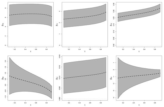
Figure 2. Athletes dataset: Point estimates (center line) and 95% confidence intervals (CIs) for model parameters under RPSN-QR model.

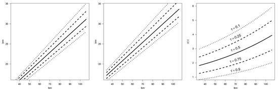
Figure 3. Data analysis: Fitted RPSN-QR model lines for the response (left panel for males, center panel for females) and scale parameter (right panel) over the grid $\tau =\{0.10,0.25,0.50,0.75,0.90\}$.

We also present in Table 4 the p-value to validate the normality hypothesis based on the Kolmogorov–Smirnov (KS; Kolmogorov, [18]) for the quantile residuals (Dunn and Smyth, [19]) using different quantile $\tau$ of such residuals. In all cases, the KS test did not reject the null hypothesis of normality. Therefore, the RPSN is appropriated to model all the quantile in this problem.

Table 4. p-values for normality K-S test for residuals under our RPSN-QR model for the athletes dataset for different quantiles $\tau$’s.

$\mathit{\tau }$	0.10	0.15	0.20	0.25	0.30	0.35	0.40	0.45	0.50
p-value	0.995	0.996	0.991	0.976	0.951	0.914	0.864	0.853	0.837
$\tau$	0.55	0.60	0.65	0.70	0.75	0.80	0.85	0.90
p-value	0.765	0.810	0.777	0.683	0.604	0.524	0.394	0.191

We also performed a local influence analysis. Figure 4 shows such analysis under the three perturbation schemes discussed in Section 3 for $\tau =0.5$. The Appendix A.2 shows the analysis for other quantiles $\tau =0.1,0.25,0.75$ and $0.9$. Note that observations 75, 162 and 178 are detected as potentially influent for all the mentioned quantiles and the observation 53 appears for the quantile $0.9$.

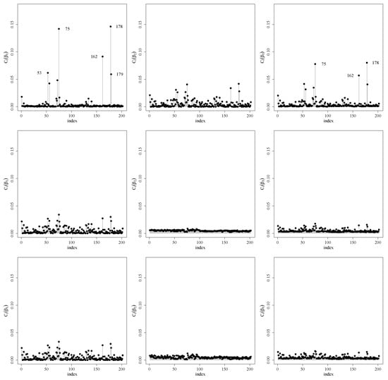
Figure 4. Index plots for $C_i({\widehat{\mathbf{\beta }}}_1)$ (left), $C_i({\widehat{\mathbf{\beta }}}_2)$ (center) and $C_i({\widehat{\mathbf{\beta }}}_3)$ (right) under the weight perturbation (upper), response perturbation (center) and covariate perturbation (lower) schemes for RPSN model for $\tau =0.5$.

To check the impact on the inference of possible influential cases, we consider the relative change (RC), which is computed by removing the possible influential cases for each parameter and its SE as

$$R{C}_{{\theta }_{j\left(i\right)}}=100\%\times \left|\frac{{\widehat{\theta }}_j-{\widehat{\theta }}_{j\left(i\right)}}{{\widehat{\theta }}_j}\right|\mathrm{and}R{C}_{SE\left({\theta }_{j\left(i\right)}\right)}=100\%\times \left|\frac{SE\left({\widehat{\theta }}_j\right)-SE\left({\widehat{\theta }}_{j\left(i\right)}\right)}{SE\left({\widehat{\theta }}_j\right)}\right|,$$

where ${\theta }_j$ is any component of the vector $\mathbf{\theta }=\mathbf{\theta }\left(\tau \right)$, where ${\widehat{\theta }}_{j\left(i\right)}$ and $SE\left({\widehat{\theta }}_{j\left(i\right)}\right)$ denote the ML estimate of ${\theta }_j$ and its corresponding SE, respectively, after dropping the i-th observation. Table 5 shows such RC for the non-intercept regression coefficients when observations 53, 75, 162 and 178 are removed. Note that the RC is greater for the estimated parameters than its estimated SE. However, the significance of ${\beta }_{11}\left(\tau \right)$ and ${\beta }_{12}\left(\tau \right)$ is maintained whereas ${\beta }_{21}\left(\tau \right)$ is not significant with a 5%. More combinations of dropped observations are presented in the Appendix A.2.

Table 5. Relative changes (RC) (in %) in ML estimates and their corresponding SE’s for the indicated parameter and respective p-values for the athletes dataset when observations 53, 75, 162 and 178 are dropped.

Dropped			$\mathit{\tau }$
Cases		Parameter	0.10	0.25	0.50	0.75	0.90
53, 75,	RC		7.20	9.06	12.56	17.82	24.05
162 and 178	RCSE	${\beta }_{11}\left(\tau \right)$	0.74	0.74	0.69	0.63	0.52
	p-value		<0.0001	<0.0001	<0.0001	<0.0001	<0.0001
	RC		1.98	5.63	10.93	17.22	23.38
	RCSE	${\beta }_{12}\left(\tau \right)$	0.47	0.26	0.20	0.34	0.42
	p-value		<0.0001	<0.0001	<0.0001	<0.0001	<0.0001
	RC		34.55	36.83	40.05	43.61	46.96
	RCSE	${\beta }_{21}\left(\tau \right)$	0.23	0.53	0.69	0.36	0.66
	p-value		0.0806	0.0762	0.0727	0.0697	0.0670

5. Concluding Remarks

Extending the quantile regression methods to include asymmetric response variables on the real line is promising area of research. In this paper, we have introduced a novel flexible parametric quantile regression model for asymmetric response variables, which can be very useful in modeling response variables on the real line at different quantiles. The proposed quantile regression model was built based on PSN distribution using a new parameterization of this distribution that is indexed by quantile, precision and shape parameters, in which a function of any quantile of the response variable is given by a linear predictor that is defined by regression parameters and explanatory variables. We consider a frequentist approach to estimate the model parameters, and the maximum likelihood inference is employed to estimate the model parameters. An application using a real dataset was presented and discussed. Results of the application showed that the model is adequate; it elaborately showed which covariates influence the response at different levels of quantiles. Finally, there are many possible extensions of the current work, for instance, mixtures of RPSN regression models in order to accommodate multimodality, a semi-parametric component to include a functional covariate to model nonlinearity of the response, and measurement errors, among others. An in-depth investigation of these topics is beyond the scope of this work, and will be considered elsewhere.

Appendix A.1. Details for Score and Hessian

For the score vector in Equation (4), the elements of the form $\frac{\partial {\ell }_i}{\partial {\xi }_i}$, with $\xi \in \{\mu ,\sigma ,\lambda \}$ are given by

$$\begin{array}{cc}\hfill \frac{\partial {\ell }_i}{\partial {\mu }_i}& =-\frac{1}{{\sigma }_i}\left\{{\lambda }_i{m}_0\left({\lambda }_i{z}_i\right)-z_i+\left[\alpha ({\lambda }_i,\tau )-1\right]m_{{\lambda }_i}\left(z_i\right)\right\},\hfill \\ \hfill \frac{\partial {\ell }_i}{\partial {\sigma }_i}& =-\frac{z_i}{{\sigma }_i}\left\{{\lambda }_i{m}_0\left({\lambda }_i{z}_i\right)-z_i+\left[\alpha ({\lambda }_i,\tau )-1\right]m_{{\lambda }_i}\left(z_i\right)\right\}-\frac{1}{{\sigma }_i},\hfill \\ \hfill \frac{\partial {\ell }_i}{\partial {\lambda }_i}& =log\left(\tau \right){\left[\alpha ({\lambda }_i,\tau )({\lambda }_i^2+1)\left(\frac{\pi }{2}-\arctan \left({\lambda }_i\right)\right)\right]}^{-1}\left(1+log{\mathsf{\Phi }}_{{\lambda }_i}\left(z_i\right)\right)\hfill \\ \hfill & +z_i{m}_0\left({\lambda }_i{z}_i\right)-\left[\alpha ({\lambda }_i,\tau )-1\right]\frac{m_0\left({\lambda }_i{z}_i\right)}{(1+{\lambda }_i^2)},\hfill \end{array}$$

where $m_{\lambda }\left(z\right)={\varphi }_{\lambda }\left(z\right)/{\mathsf{\Phi }}_{\lambda }\left(z\right)$.

For the Hessian in Equation (5), the elements of the form ${\partial }^2{\ell }_i/\partial {\xi }_i\partial {\xi }_i^{{}^{\prime }}$, with $\xi ,{\xi }^{{}^{\prime }}\in \{\mu ,\sigma ,\lambda \}$ are given by

$$\begin{array}{cc}\hfill \frac{{\partial }^2{\ell }_i}{\partial {\mu }_i^2}& =\frac{1}{{\sigma }_i^2}\left\{{\lambda }_i^2{m}_0^{{}^{\prime }}\left({\lambda }_i{z}_i\right)-1+[\alpha ({\lambda }_i,\tau )-1]m_{{\lambda }_i}^{{}^{\prime }}\left(z_i\right)\right\}\hfill \\ \hfill \frac{{\partial }^2{\ell }_i}{\partial {\mu }_i\partial {\sigma }_i}& =\frac{z_i}{{\sigma }_i}\left\{{\lambda }_i^2{m}_0^{{}^{\prime }}\left({\lambda }_i{z}_i\right)-1+[\alpha ({\lambda }_i,\tau )-1]m_{{\lambda }_i}^{{}^{\prime }}\left(z_i\right)\right\}\hfill \\ \hfill \frac{{\partial }^2{\ell }_i}{\partial {\mu }_i\partial {\lambda }_i}& =-\frac{1}{{\sigma }_i}\{\frac{log\left(\tau \right)m_{\lambda }\left(z_i\right)}{(1+{\lambda }_i^2)\left(\frac{\pi }{2}-\arctan \left({\lambda }_i\right)\right)\left(1+log{\mathsf{\Phi }}_{{\lambda }_i}\left(z_i\right)\right)}+m\left({\lambda }_i{z}_i\right)+{\lambda }_i{z}_i{m}_0^{{}^{\prime }}\left({\lambda }_i{z}_i\right)\hfill \\ \hfill & -\frac{[\alpha ({\lambda }_i,\tau )-1]{\lambda }_i{m}_0^{{}^{\prime }}\left({\lambda }_i{z}_i\right)}{(1+{\lambda }_i^2)}\}\hfill \\ \hfill \frac{{\partial }^2{\ell }_i}{\partial {\sigma }_i^2}& =\frac{z_i}{{\sigma }_i^2}\left\{{\lambda }_i^2{m}_0^{{}^{\prime }}\left({\lambda }_i{z}_i\right)-1+[\alpha ({\lambda }_i,\tau )-1]m_{{\lambda }_i}^{{}^{\prime }}\left(z_i\right)\right\}+\frac{1}{{\sigma }_i^2}\hfill \\ \hfill \frac{{\partial }^2{\ell }_i}{\partial {\sigma }_i\partial {\lambda }_i}& =-\frac{z_i}{{\sigma }_i}\{\frac{log\left(\tau \right)m_{\lambda }\left(z_i\right)}{(1+{\lambda }_i^2)\left(\frac{\pi }{2}-\arctan \left({\lambda }_i\right)\right)\left(1+log{\mathsf{\Phi }}_{{\lambda }_i}\left(z_i\right)\right)}+m\left({\lambda }_i{z}_i\right)+{\lambda }_i{z}_i{m}_0^{{}^{\prime }}\left({\lambda }_i{z}_i\right)\hfill \\ \hfill & -\frac{[\alpha ({\lambda }_i,\tau )-1]{\lambda }_i{m}_0^{{}^{\prime }}\left({\lambda }_i{z}_i\right)}{(1+{\lambda }_i^2)}\}\hfill \\ \hfill \frac{{\partial }^2{\ell }_i}{\partial {\lambda }_i^2}& =\frac{{log}^2\left(\tau \right)\left[(1-\pi \lambda +2{\lambda }_i\arctan \left({\lambda }_i\right))log\left(\frac{1}{2}-\frac{1}{\pi }\arctan \left({\lambda }_i\right)\right)+1\right]\left(1+log{\mathsf{\Phi }}_{{\lambda }_i}\left(z_i\right)\right)}{{\left[\alpha ({\lambda }_i,\tau )(1+{\lambda }_i^2)\left(\frac{\pi }{2}-\arctan \left({\lambda }_i\right)\right)\right]}^2}\hfill \\ \hfill & -\frac{log\left(\tau \right)m_0\left({\lambda }_i{z}_i\right)m_{{\lambda }_i}\left(z_i\right)}{\alpha ({\lambda }_i,\tau ){(1+{\lambda }_i^2)}^2\left(\frac{\pi }{2}-\arctan \left({\lambda }_i\right)\right)(1+log{\mathsf{\Phi }}_{{\lambda }_i}\left(z_i\right))}+z_i^2{m}_0^{{}^{\prime }}\left({\lambda }_i{z}_i\right)\hfill \\ \hfill & -\frac{m\left({\lambda }_i{z}_i\right)}{log\left(\tau \right){\alpha }^2({\lambda }_i,\tau ){(1+{\lambda }_i^2)}^2\left(\frac{\pi }{2}-\arctan \left({\lambda }_i\right)\right)}\hfill \\ \hfill & -\frac{[\alpha ({\lambda }_i,\tau )-1]}{(1+{\lambda }_i^2)}\left\{z_i{m}^{{}^{\prime }}\left({\lambda }_i{z}_i\right)-2\frac{{\lambda }_{i}m\left({\lambda }_i{z}_i\right)}{(1+{\lambda }_i^2)}\right\},\hfill \end{array}$$

where $m_{\lambda }^{{}^{\prime }}\left(z\right)=\lambda m_0\left(\lambda z\right)m_{\lambda }\left(z\right)-z{m}_{\lambda }\left(z\right)-m_{\lambda }^2\left(z\right)$.

Appendix A.2. Local Influence

In this section, we present additional information for the local influence analysis in the Athletes dataset discussed in Section 5.

Figure A1. Index plots for $C_i({\widehat{\mathbf{\beta }}}_1)$ (left), $C_i({\widehat{\mathbf{\beta }}}_2)$ (center) and $C_i({\widehat{\mathbf{\beta }}}_3)$ (right) under the weight perturbation (upper), response perturbation (center) and covariate perturbation (lower) schemes for RPSN model for $\tau =0.1$.

Figure A2. Index plots for $C_i\left({\widehat{\mathbf{\beta }}}_1\right)$ (left), $C_i\left({\widehat{\mathbf{\beta }}}_2\right)$ (center) and $C_i\left({\widehat{\mathbf{\beta }}}_3\right)$ (right) under the weight perturbation (upper), response perturbation (center) and covariate perturbation (lower) schemes for RPSN model for $\tau =0.25$.

Figure A3. Index plots for $C_i\left({\widehat{\mathbf{\beta }}}_1\right)$ (left), $C_i\left({\widehat{\mathbf{\beta }}}_2\right)$ (center) and $C_i\left({\widehat{\mathbf{\beta }}}_3\right)$ (right) under the weight perturbation (upper), response perturbation (center) and covariate perturbation (lower) schemes for RPSN model for $\tau =0.75$.

Figure A4. Index plots for $C_i\left({\widehat{\mathbf{\beta }}}_1\right)$ (left), $C_i\left({\widehat{\mathbf{\beta }}}_2\right)$ (center) and $C_i\left({\widehat{\mathbf{\beta }}}_3\right)$ (right) under the weight perturbation (upper), response perturbation (center) and covariate perturbation (lower) schemes for RPSN model for $\tau =0.9$.

Table A1. RCs (in %) in ML estimates and their corresponding SEs for the indicated parameter and respective p-values for the athletes dataset when observation 75 and 178 are dropped separately.

Dropped			$\mathit{\tau }$
Cases		Parameter	0.10	0.25	0.50	0.75	0.90
75	RC		5.31	7.22	10.82	16.2	22.57
	RCSE	${\beta }_{11}\left(\tau \right)$	0.23	0.20	0.17	0.11	0.04
	p-value		<0.0001	<0.0001	<0.0001	<0.0001	<0.0001
	RC		1.82	5.03	10.02	16.09	22.08
	RCSE	${\beta }_{12}\left(\tau \right)$	0.15	0.05	0.08	0.07	0.17
	p-value		<0.0001	<0.0001	<0.0001	<0.0001	<0.0001
	RC		6.77	9.84	14.27	19.20	23.84
	RCSE	${\beta }_{21}\left(\tau \right)$	0.65	0.93	1.05	0.71	0.33
	p-value		0.0118	0.0105	0.0095	0.0086	0.0078
178	RC		0.72	2.62	6.30	11.88	18.50
	RC${}_{SE}$	${\beta }_{11}\left(\tau \right)$	0.17	0.15	0.12	0.07	0.00
	p-value		<0.0001	<0.0001	<0.0001	<0.0001	<0.0001
	RC		0.12	3.36	8.60	14.88	21.06
	RC${}_{SE}$	${\beta }_{12}\left(\tau \right)$	0.13	0.06	0.09	0.07	0.18
	p-value		<0.0001	<0.0001	<0.0001	<0.0001	<0.0001
	RC		22.91	25.43	29.09	33.17	37.01
	RC${}_{SE}$	${\beta }_{21}\left(\tau \right)$	0.75	0.47	0.31	0.61	1.61
	p-value		0.0449	0.0418	0.0393	0.0371	0.0352

Table A1. RCs (in %) in ML estimates and their corresponding SEs for the indicated parameter and respective p-values for the athletes dataset when observation 75 and 178 are dropped separately.

Dropped			$\mathit{\tau }$
Cases		Parameter	0.10	0.25	0.50	0.75	0.90
75	RC		5.31	7.22	10.82	16.2	22.57
	RCSE	${\beta }_{11}\left(\tau \right)$	0.23	0.20	0.17	0.11	0.04
	p-value		<0.0001	<0.0001	<0.0001	<0.0001	<0.0001
	RC		1.82	5.03	10.02	16.09	22.08
	RCSE	${\beta }_{12}\left(\tau \right)$	0.15	0.05	0.08	0.07	0.17
	p-value		<0.0001	<0.0001	<0.0001	<0.0001	<0.0001
	RC		6.77	9.84	14.27	19.20	23.84
	RCSE	${\beta }_{21}\left(\tau \right)$	0.65	0.93	1.05	0.71	0.33
	p-value		0.0118	0.0105	0.0095	0.0086	0.0078
178	RC		0.72	2.62	6.30	11.88	18.50
	RC${}_{SE}$	${\beta }_{11}\left(\tau \right)$	0.17	0.15	0.12	0.07	0.00
	p-value		<0.0001	<0.0001	<0.0001	<0.0001	<0.0001
	RC		0.12	3.36	8.60	14.88	21.06
	RC${}_{SE}$	${\beta }_{12}\left(\tau \right)$	0.13	0.06	0.09	0.07	0.18
	p-value		<0.0001	<0.0001	<0.0001	<0.0001	<0.0001
	RC		22.91	25.43	29.09	33.17	37.01
	RC${}_{SE}$	${\beta }_{21}\left(\tau \right)$	0.75	0.47	0.31	0.61	1.61
	p-value		0.0449	0.0418	0.0393	0.0371	0.0352

Table A2. RCs (in %) in ML estimates and their corresponding SEs for the indicated parameter and respective p-values for the athletes dataset when observations {75, 178} and {75, 162, 178} are dropped separately.

Dropped			$\mathit{\tau }$
Cases		Parameter	0.10	0.25	0.50	0.75	0.90
75 and	RC		6.30	8.16	11.69	17.01	23.29
178	RCSE	${\beta }_{11}\left(\tau \right)$	0.41	0.39	0.34	0.28	0.19
	p-value		<0.0001	<0.0001	<0.0001	<0.0001	<0.0001
	RC		1.75	5.32	10.58	16.84	22.97
	RCSE	${\beta }_{12}\left(\tau \right)$	0.29	0.08	0.03	0.18	0.27
	p-value		<0.0001	<0.0001	<0.0001	<0.0001	<0.0001
	RC		31	33.34	36.67	40.38	43.87
	RCSE	${\beta }_{21}\left(\tau \right)$	0.04	0.27	0.42	0.11	0.91
	p-value		0.0674	0.0633	0.0600	0.0572	0.0546
75, 162	RC		5.43	7.27	10.80	16.13	22.45
and 178	RCSE	${\beta }_{11}\left(\tau \right)$	0.57	0.54	0.50	0.43	0.34
	p-value		<0.0001	<0.0001	<0.0001	<0.0001	<0.0001
	RC		1.36	5.12	10.53	16.91	23.14
	RCSE	${\beta }_{12}\left(\tau \right)$	0.39	0.18	0.12	0.26	0.35
	p-value		<0.0001	<0.0001	<0.0001	<0.0001	<0.0001
	RC		43.37	45.46	48.35	51.53	54.51
	RCSE	${\beta }_{21}\left(\tau \right)$	0.29	0.61	0.77	0.46	0.56
	p-value		0.1300	0.1251	0.1212	0.1178	0.1149

Table A2. RCs (in %) in ML estimates and their corresponding SEs for the indicated parameter and respective p-values for the athletes dataset when observations {75, 178} and {75, 162, 178} are dropped separately.

Dropped			$\mathit{\tau }$
Cases		Parameter	0.10	0.25	0.50	0.75	0.90
75 and	RC		6.30	8.16	11.69	17.01	23.29
178	RCSE	${\beta }_{11}\left(\tau \right)$	0.41	0.39	0.34	0.28	0.19
	p-value		<0.0001	<0.0001	<0.0001	<0.0001	<0.0001
	RC		1.75	5.32	10.58	16.84	22.97
	RCSE	${\beta }_{12}\left(\tau \right)$	0.29	0.08	0.03	0.18	0.27
	p-value		<0.0001	<0.0001	<0.0001	<0.0001	<0.0001
	RC		31	33.34	36.67	40.38	43.87
	RCSE	${\beta }_{21}\left(\tau \right)$	0.04	0.27	0.42	0.11	0.91
	p-value		0.0674	0.0633	0.0600	0.0572	0.0546
75, 162	RC		5.43	7.27	10.80	16.13	22.45
and 178	RCSE	${\beta }_{11}\left(\tau \right)$	0.57	0.54	0.50	0.43	0.34
	p-value		<0.0001	<0.0001	<0.0001	<0.0001	<0.0001
	RC		1.36	5.12	10.53	16.91	23.14
	RCSE	${\beta }_{12}\left(\tau \right)$	0.39	0.18	0.12	0.26	0.35
	p-value		<0.0001	<0.0001	<0.0001	<0.0001	<0.0001
	RC		43.37	45.46	48.35	51.53	54.51
	RCSE	${\beta }_{21}\left(\tau \right)$	0.29	0.61	0.77	0.46	0.56
	p-value		0.1300	0.1251	0.1212	0.1178	0.1149

References

- Azzalini, A. A class of distributions which includes the normal ones. Scand. J. Stat. 1985, 12, 171–178. [Google Scholar]
- Azzalini, A. Further results on a class of distributions which includes the normal ones. Statistica 1986, 46, 199–208. [Google Scholar]
- Arellano-Valle, R.B.; Gómez, H.W.; Quintana, F.A. A New Class of Skew-Normal Distributions. Commun. Stat. Theory Methods 2004, 33, 1465–1480. [Google Scholar] [CrossRef]
- Pewsey, A.; Gómez, H.W.; Bolfarine, H. Likelihood-based inference for power distributions. Test 2012, 21, 775–789. [Google Scholar] [CrossRef]
- Lehmann, E.L. The power of rank tests. Ann. Math. Statist. 1953, 24, 23–43. [Google Scholar] [CrossRef]
- Durrans, S.R. Distributions of fractional order statistics in hydrology. Water Resour. Res. 1992, 28, 1649–1655. [Google Scholar] [CrossRef]
- Gupta, D.; Gupta, R.C. Analyzing skewed data by power normal model. Test 2008, 17, 197–210. [Google Scholar] [CrossRef]
- Castillo, N.O.; Gallardo, D.I.; Bolfarine, H.; Gómez, H.W. Truncated power-normal distribution with application to non-negative measurements. Entropy 2018, 20, 433. [Google Scholar] [CrossRef]
- Martínez-Flórez, G.; Arnold, B.C.; Bolfarine, H.; Gómez, H.W. The alpha-power tobit model. Commun. Stat. Theory Methods 2013, 42, 633–643. [Google Scholar] [CrossRef]
- Martínez-Flórez, G.; Bolfarine, H.; Gómez, H.W. Doubly censored power-normal regression models with inflation. Test 2015, 24, 265–286. [Google Scholar] [CrossRef]
- Martínez-Flórez, G.; Bolfarine, H.; Gómez, H.W. Skew-normal alpha-power model. Statistics 2014, 48, 1414–1428. [Google Scholar] [CrossRef]
- Martínez-Flórez, G.; Bolfarine, H.; Gómez, H.W. The log alpha-power asymmetric distribution with application to air pollution. Environmetrics 2014, 25, 44–56. [Google Scholar] [CrossRef]
- Martínez-Flórez, G.; Bolfarine, H.; Gómez, H.W. Asymmetric regression models with limited responses with an application to antibody response to vaccine. Biom. J. 2013, 55, 156–172. [Google Scholar] [CrossRef] [PubMed]
- Cook, R.D. Detection of influential observation in linear regression. Technometrics 1977, 19, 15–18. [Google Scholar]
- Cook, R.D.; Weisberg, S. An Introduction to Regression Graphics; Wiley: New York, NY, USA, 1994. [Google Scholar]
- Galarza, C.E.; Lachos, V.H.; Barbosa, C.; Castro, L.M. Robust quantile regression using a generalized class of skewed distributions. Stat 2017, 6, 113–130. [Google Scholar]
- Akaike, H. A new look at the statistical model identification. IEEE Trans. Autom. Control 1974, 19, 716–723. [Google Scholar] [CrossRef]
- Kolmogorov, A.N. Sulla determinazione empirica di una legge di distribuzionc. Giorn. Ist. Ital. Attuar. 1933, 4, 83–91. [Google Scholar]
- Dunn, P.; Smyth, G. Randomized quantile residuals. J. Comput. Graph. Stat. 1996, 5, 236–244. [Google Scholar]
Publisher’s Note: MDPI stays neutral with regard to jurisdictional claims in published maps and institutional affiliations. |
© 2020 by the authors. Licensee MDPI, Basel, Switzerland. This article is an open access article distributed under the terms and conditions of the Creative Commons Attribution (CC BY) license (http://creativecommons.org/licenses/by/4.0/).