Image Denoising Based on Bivariate Distribution

Abstract

The literature has shown that the performance of the de-noising algorithm was greatly influenced by the dependencies between wavelet coefficients. In this paper, the bivariate probability density function (PDF) was proposed which was symmetric, and the dependencies between the coefficients were considered. The bivariate Cauchy distribution and the bivariate Student’s distribution are special cases of the proposed bivariate PDF. One of the parameters in the probability density function gave the estimation method, and the other parameter can take any real number greater than 2. The algorithm adopted a maximum a posteriori estimator employing the dual-tree complex wavelet transform (DTCWT). Compared with the existing best results, the method is faster and more efficient than the previous numerical integration techniques. The bivariate shrinkage function of the proposed algorithm can be expressed explicitly. The proposed method is simple to implement.

1. Introduction

Image denoising is very important in many image processing applications. The methods of de-noising using wavelet transform have been widely proposed. Chang et al. proposed a subband adaptive method based on the generalized Gaussian distribution (GGD) model in [1]. Mihçak et al. in [2] gave the Bayesian linear least mean square error estimation (LMMSE) method by using the central square window. Portiilla et al. in [3] proposed a stochastic model by a hidden random field with an overcomplete wavelet pyramid. In [4], the method of combining dual tree complex wavelet with total variation is studied to eliminate speckle noise and Gaussian noise in ultrasonic image. In [5], a threshold estimation denoising method based on double density wavelet transform (DDWT) was proposed. Shen et al. in [6] proposed a denoising algorithm by constructing nonseparable Parseval frames. The paper in [7] used the designed tight frame wavelet filters for image de-noising.

The de-noising method can effectively improve the processing performance by considering the dependence between wavelet subbands. Senduer and Selesnick in [8,9] have developed a new non-Gaussian bivariate distribution, and a scheme was developed which considers the statistical dependency between the dual-tree complex wavelet coefficients.Achim et al. in [10] designed a bivariate Bayesian estimator using bivariate $\alpha$-stable distributions. A spatially adaptive method had been introduced using the Cauchy Prior for the speckle reduction in [11,12], and developed method using Gaussian probability density function (PDF) in [13] by Bhuiyan et al., respectively. Ranjani and Thiruvengadam in [14,15] proposed a despeckling algorithm using the bivariate Cauchy probability density function (PDF) by the DTCWT subbands, respectively. In [16], a denoising speckle algorithm was proposed using a heavy tailed Levy distribution based on DTCWT for the ultrasound images. A denoising algorithm was developed using scale mixtures of Rayleigh distribution in [17]. The dual-tree complex wavelet (DTCWT) is tight frame wavelet in [18,19]. The DTCWT have advantages that orthogonal bases can not have for image de-noising [20,21,22].

In this paper, a bivariate symmetric probability density function (PDF) was proposed, which utilizes the dependence of DTCWT wavelet coefficients of each subband. A novel noise reduction algorithm has been introduced for noisy images.

The organization of this paper is as follows. Section 2 describes a noise reduction algorithm. The expression of the parameter for the distribution in each wavelet subband is also derived. The standard maximum posterior (map) estimation of undamaged wavelet coefficients is given in Section 2. The experimental results of the proposed method are discussed in Section 3. Finally, conclusions are given in Section 4.

2. Proposed Algorithm

The paper discusses the denoising of the image with additive white Gaussian noise. Let ${\omega }_{1k}$ represent the kth wavelet coefficient, and ${\omega }_{2k}$ represent the wavelet coefficient at the next scale. $y_{1k}$ and $y_{2k}$ are noisy observations of ${\omega }_{1k}$ and ${\omega }_{2k}$, and $n_{1k}$ and $n_{2k}$ are noise samples.

$${\mathbf{y}}_k={\mathbf{w}}_k+{\mathbf{n}}_k$$

(1)

where ${\mathbf{w}}_k=\left(w_{1,k},w_{2,k}\right)$, ${\mathbf{y}}_k=\left(y_{1,k},y_{2,k}\right)$, and ${\mathbf{n}}_k=\left(n_{1,k},n_{2,k}\right)$ in the wavelet domain. To improve readability, the coefficient index k is omitted. In this paper, we proposed a joint bivariate PDF as

$$f_{\mathbf{w}}\left(w_1,w_2\right)=\frac{\theta {\gamma }^{\theta }}{2\pi {\left({\gamma }^2+w_1^2+w_2^2\right)}^{\frac{\theta +2}{2}}},\theta >0$$

(2)

where $\gamma$ is the dispersion parameter. The joint bivariate symmetric probability density function (PDF) for the coefficients was illustrated in Figure 1.

In the previous literature, most of the exponential functions were used as densities for noise removal [8,9,13,16], and the exponential functions attenuated rapidly. The density of this paper is composed of power functions when the parameter $\theta$ is given.

The density of this paper was composed of power functions when the parameter $\theta$ was given. The attenuation speed of power functions is relatively slow and the density has a thick tail. We know that most of the practical application problems have thick tails. The density function of this paper is more consistent with the actual problems and is more conducive to dealing with practical problems. The bivariate Cauchy distribution and the bivariate student’s distribution are special cases of the bivariate PDF in (2).

The value of parameter $\theta$ in (2) has a relatively large influence on the experimental results. Different kinds of image corresponding $\theta$ values have different noising effects. For example, this paper used $\theta =4$ to reduce boat image noise. When $\theta =4$, the marginal probability density function of bivariate PDF $f_{\mathbf{w}}\left(w_1,w_2\right)$ is calculated as follows

$$f_{w_1}\left(x\right)=\frac{4{\gamma }^4}{\pi }{\int }_0^{+\infty }\frac{1}{{\left({\gamma }^2+x^2+y^2\right)}^3}dy.$$

(3)

Using the following identity in [23]

$${\int }_0^{+\infty }\frac{y^{\mu -1}}{{\left(p+q{y}^v\right)}^{n+1}}dy=\frac{1}{v{p}^{n+1}}{\left(\frac{p}{q}\right)}^{\frac{\mu }{v}}\frac{\Gamma \left(\frac{\mu }{v}\right)\Gamma \left(n+1-\frac{\mu }{v}\right)}{\Gamma \left(n+1\right)}.$$

(4)

The solution of integral in (3) is as

$$f_{w_1}\left(x\right)=\frac{2{\gamma }^4}{\pi }\frac{\Gamma \left(\frac{1}{2}\right)\Gamma \left(\frac{5}{2}\right)}{\Gamma \left(3\right)}\frac{1}{{\left({\gamma }^2+x^2\right)}^{\frac{5}{2}}}$$

(5)

where the gamma function

$$\Gamma \left(t\right)={\int }_0^{+\infty }{x}^{t-1}{e}^{-t}dx.$$

Similarly, the marginal density of $w_2$ can be obtained. Because the product of two marginal densities is not equal to the joint density, this indicates that $w_1$ and $w_2$ are dependent. To motivate this model, see Figure 2. The solid line showed the fitted curve of the original high-band coefficients of boat image from the first scale, obtained by employing and the marginal PDF in (5) and DTCWT in [8], and the dispersion parameter $\gamma$ values for $\theta =4$ were estimated by local marginal standard deviations $\sigma$ rearranging (7) which are described later. The dashed line shows the fitted curve by Gaussian probability density function (PDF). Observe that the normalized histogram is well approximated by the marginal PDF of the bivariate PDF in (5).

The independent bivariate Gaussian PDF of noise ${\mathbf{n}}_k$ is.

$$f_{{\mathbf{n}}_k}\left(n_1,n_2\right)=\frac{1}{2\pi {\sigma }_n^2}exp(-\frac{n_1^2+n_2^2}{2{\sigma }_n^2})$$

(6)

where ${\sigma }_n^2$ is the variance of Gaussian noise.

The parameters $\gamma$ for the bivariate PDF in (2) are calculated using the marginal variance ${\sigma }^2$ of the kth wavelet coefficient as

$${\sigma }^2=D\left(w_1\right)={\int }_{-\infty }^{+\infty }{\int }_{-\infty }^{+\infty }\frac{\theta {\gamma }^{\theta }{w}_1^2}{2\pi {({\gamma }^2+w_1^2+w_2^2)}^{\frac{\theta +2}{2}}}d{w}_{1}d{w}_2=\frac{{\gamma }^2}{\theta -2}$$

(7)

where $\theta >2$. When $\theta \le 2$, the marginal variance does not exist.

The local marginal variance ${\sigma }^2$ of the kth coefficient is calculated using the central square window $\Lambda$ as the following [8]

$${\widehat{\sigma }}^2=max(0,\frac{1}{N_{\Lambda }}\sum _{y_1\in \Lambda }{y}_1^2-{\widehat{\sigma }}_n^2)$$

(8)

where $N_{\Lambda }$ is number of points in window $\Lambda$, ${\sigma }_n^2$ be the noise marginal variance.

The estimator in [24] is used to estimate the noise variance ${\sigma }_n^2$

$${\widehat{\sigma }}_n=\frac{\mathrm{median} \left(\left|y_j\right|\right)}{0.6745},y_j\in \mathrm{subband} \mathrm{HH}.$$

(9)

Rearranging (7), the estimator of the parameter $\gamma$ for the bivariate PDF is derived as

$${\widehat{\gamma }}^2=(\theta -2)max(0,\frac{1}{N_{\Lambda }}\sum _{y_1\in \Lambda }{y}_1^2-{\widehat{\sigma }}_n^2).$$

(10)

The standard maximum a posteriori (MAP) estimator of w for the observation y is

$$\widehat{\mathbf{w}}=\underset{\mathbf{w}}{argmax}p\left(\mathbf{w}\right|\mathbf{y}).$$

(11)

It is just sufficient to maximize $p_{\mathbf{n}}\left(\mathbf{y}\right|\mathbf{w})p_{\mathbf{w}}\left(\mathbf{w}\right)$

$$\begin{gathered} \widehat{\mathbf{w}}=\underset{\mathbf{w}}{argmax}\left[p_{\mathbf{n}}\left(\mathbf{y}\right|\mathbf{w})p_{\mathbf{w}}\left(\mathbf{w}\right)\right] \\ =\underset{\mathbf{w}}{argmax}\left[p_{\mathbf{n}}(\mathbf{y}-\mathbf{w})p_{\mathbf{w}}\left(\mathbf{w}\right)\right]. \end{gathered}$$

(12)

The MAP estimator in (2) can also be calculated as

$$\widehat{\mathbf{w}}=\underset{\mathbf{w}}{argmax}[log{p}_{\mathbf{n}}(\mathbf{y}-\mathbf{w})+log{p}_{\mathbf{w}}\left(\mathbf{w}\right)].$$

(13)

The probability density functions of signal and noise defined in (2) and (6) are substituted into (13), respectively, we get

$$\widehat{\mathbf{w}}=\underset{\mathbf{w}}{argmax}\left[L(w_1,w_2)\right]$$

(14)

where

$$L(w_1,w_2)=-\frac{{(y_1-w_1)}^2+{(y_2-w_2)}^2}{2{\sigma }_n^2}-\frac{\theta +2}{2}log({\gamma }^2+w_1^2+w_2^2)$$

The solution to (14) can be obtained by solving the following equations:

$$\frac{\partial L(w_1,w_2)}{\partial w_1}=\frac{y_1-w_1}{{\sigma }_n^2}-(\theta +2)\frac{w_1}{{\gamma }^2+w_1^2+w_2^2}=0$$

(15)

$$\frac{\partial L(w_1,w_2)}{\partial w_2}=\frac{y_2-w_2}{{\sigma }_n^2}-(\theta +2)\frac{w_2}{{\gamma }^2+w_1^2+w_2^2}=0$$

(16)

Rearranging (15) and (16), we get $w_2=w_1{y}_2/\phantom{y_2{y}_1}{y}_1$, and by substituting $w_2$ into (15), it is rewritten as

$$\left(y_1^2+y_2^2\right)w_1^3-y_1\left(y_1^2+y_2^2\right)w_1^2+\left[{\gamma }^2{y}_1^2+(\theta +2){\sigma }_n^2{y}_1^2\right]w_1-{\gamma }^2{y}_1^3=0.$$

(17)

According to the method of [25], the real solution of the cubic equation in Equation (17) is as follows

$$w_1=\frac{y_1}{3}+\sqrt[3]{-p+\sqrt{p^2+q^3}}{y}_1+\sqrt[3]{-p-\sqrt{p^2+q^3}}{y}_1$$

(18)

where

$$p=\frac{-18{\gamma }^2+9(\theta +2){\sigma }_n^2}{54\left(y_1^2+y_2^2\right)}-\frac{1}{27}$$

$$q=\frac{{\gamma }^2+(\theta +2){\sigma }_n^2}{3\left(y_1^2+y_2^2\right)}-\frac{1}{9}.$$

The shrinkage function is obtained as following

$${\widehat{w}}_1=(\frac{1}{3}+\sqrt[3]{-p+\sqrt{p^2+q^3}}+\sqrt[3]{-p-\sqrt{p^2+q^3}})+y_1$$

(19)

where ${\left(g\right)}_{+}$ is defined as

$${\left(g\right)}_{+}=\left\{\begin{array}{c} 0,\mathrm{if}g<0\hfill \\ g,\mathrm{otherwise}.\hfill \end{array}\right.$$

Figure 3 showed the bivariate shrinkage function figure in (19), as shown in the figure, there was a dead zone (the dead zone is the area where the estimate is zero), that is,

$$\mathrm{deadzone}=\left\{(y_1,y_2):\frac{1}{3}+\sqrt[3]{-p+\sqrt{p^2+q^3}}+\sqrt[3]{-p-\sqrt{p^2+q^3}}\le 0\right\}.$$

The denoising image was obtained by inverse DTCWT of the estimated wavelet coefficients by (19). The block diagram showing the proposed de-noising process steps was given in Figure 4.

The denoising algorithm is described as follows:

(1)

First implement the DTCWT to get ${\mathbf{y}}_k$.

(2)

Calculate ${\widehat{\sigma }}_n^2$ using Equation (9).

(3)

Estimate marginal variance ${\sigma }^2$ using Equation (8).

(4)

Calculate the parameter ${\widehat{\gamma }}^2$ using Equation (10).

(5)

Estimate the $w_1$ using Equation (19) with the $L\times L$ local window.

(6)

Reconstruct the estimated image by ${\widehat{w}}_1$.

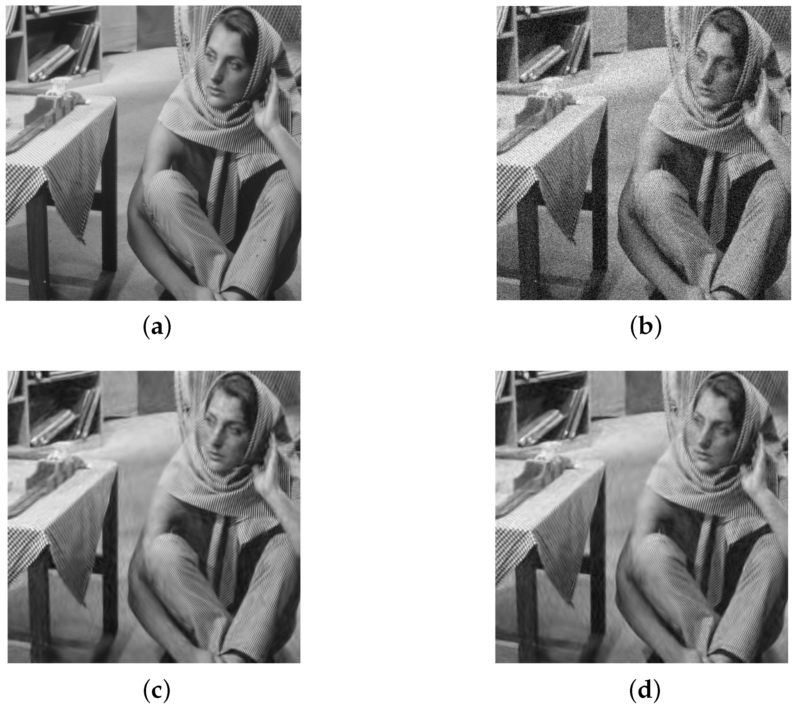
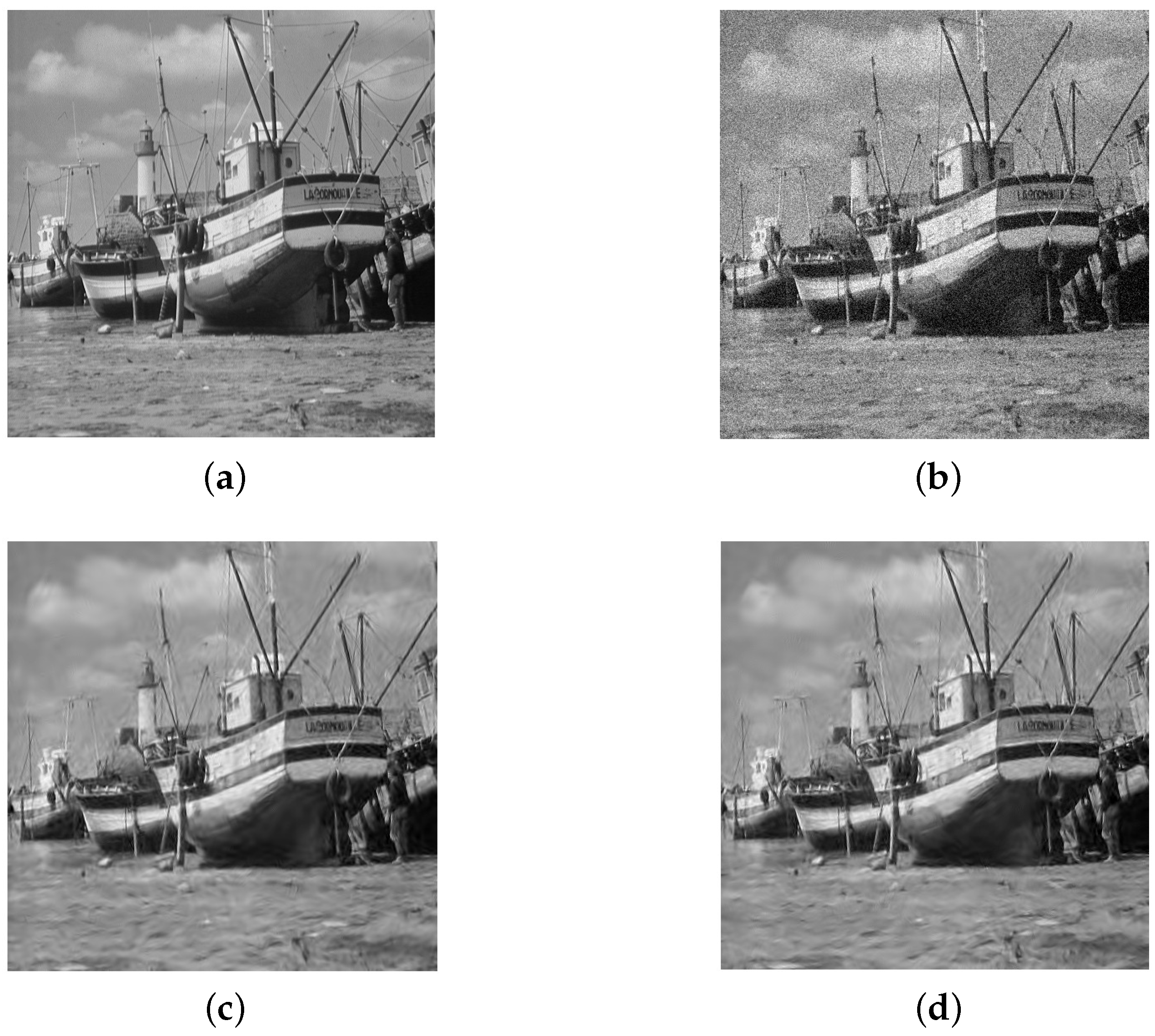
3. Experimental Results

In the experiments, the proposed density is used to give the algorithm, and it is compared with other famous image restoration models such as using Gaussian probability density function (PDF) [2], using the GSM (Gaussian scale mixture) algorithm [3], using non Gaussian probability density function (PDF) [8], using the tight frame in [6]. The results show that the denoising effect of the new model is effective compared with the above methods.

Table 1. Peak signal-to-noise ratio values of denoised images different test images and noise levels (${\sigma }_n)$ of noisy.

	Noisy	Method in [2]	Method in [6]	Method in [3]	Method in [8]	Proposed Method
Barbara
${\sigma }_n=10$	28.13	31.96	32.73	34.03	33.29	33.4417
${\sigma }_n=15$	24.61	29.57	30.56	31.86	31.17	31.3435
${\sigma }_n=20$	22.11	27.91	28.80	30.32	29.66	29.8558
${\sigma }_n=25$	20.17	26.72	27.45	29.13	28.52	28.7222
${\sigma }_n=30$	18.59	25.77	26.36	28.10	27.61	27.8130
boat
${\sigma }_n=10$	28.13	32.22	33.20	33.58	32.99	33.1018
${\sigma }_n=15$	24.61	30.37	31.61	31.70	31.23	31.3226
${\sigma }_n=20$	22.11	28.97	30.28	30.38	29.94	30.0276
${\sigma }_n=25$	20.17	27.88	29.17	29.37	28.93	29.0215
${\sigma }_n=30$	18.59	27.03	28.14	28.51	28.12	28.2095
Lena
${\sigma }_n=10$	28.13	34.07	34.92	35.61	35.29	35.3183
${\sigma }_n=15$	24.61	32.20	33.24	33.90	33.57	33.5090
${\sigma }_n=20$	22.11	30.86	31.99	32.66	32.33	32.2410
${\sigma }_n=25$	20.17	29.86	31.00	31.69	31.35	31.2753
${\sigma }_n=30$	18.59	29.02	30.14	30.91	30.54	30.4862

show the performance of the proposed algorithm and other literature methods. The peak signal-to-noise ratio(PSNR) is used to test the performance of these algorithms. To do this, we use different noise levels ${\sigma }_n^2$ for the Barbara, boat, Lena images.

Let $s,d$ represent the original image and the denoised image. The root mean-square (rms) error is determined by

$$rms=\sqrt{\frac{1}{N}\sum _k{\left(s_k-d_k\right)}^2}$$

(20)

where N is the number of pixels. The PSNR is determined by

$$\mathrm{PSNR}=20{log}_{10}\left(\frac{255}{\mathrm{rms}}\right).$$

(21)

The proposed algorithm in this paper uses the filter in [8] and the DTCWT in [18,19], which are tabulated in “ Proposed-Method" column of Table 1. The number of decomposition levels is 5, using $7\times 7$ window size $N_{\Lambda }$. The parameter $\theta$ of the shrinkage function in (19) affects the noising effect. As the parameter $\theta$ values are manually selected prior to running a simulation, the user may have to experiment with different values to achieve the highest increase in noise removal effect. In our experiments, the parameter $\theta$ takes 11 when the standard deviation ${\sigma }_n=10,15$, and $\theta$ takes 3 when the standard deviation ${\sigma }_n=20,25,30$ for lena image. The parameter $\theta$ takes 11 for all noise levels of the Barbara image, and the parameter $\theta$ takes 4 for all noise levels of the Boat image. The PSNR is the average value of the data obtained by running 100 times the proposed algorithm. We also compare the algorithm with other methods reported in the literature. Here, we give the results compared with the other four methods. In Table 1, the PSNR values using the denoising algorithm in [2] with the exponential prior are tabulated in “Method in [2]” column, the PSNR values using the GSM (Gaussian scale mixture) algorithm described in [3] are tabulated in “Method in [3]” column, the PSNR values with the DTCWT in [8] are tabulated in “Method in [8]” column, and the PSNR values with the tight frame in [6] are tabulated in “Method in [6]” column, separately. We indeed found out that a new model improves the denoising performance. In [8], the Matlab implementation for that algorithm takes 25 s for a 512 × 512 image on 450-MHz Pentium II, the Matlab program for the proposed algorithm takes 2.51 s for a 512 × 512 image on core(TM) i3 M 350.

The denoised image using a $512\times 512$ Barbara image is shown in Figure 5. The original and the noisy images are shown in Figure 5a,b. The denoised image using the method in [8] was illustrated in Figure 5c and had PSNR value of 28.52 dB, and the denoised image using the proposed method was illustrated in Figure 5d and had PSNR value of 28.7222 dB, with the Gaussian noise standard deviation 25, respectively. Other denoised image using a $512\times 512$ boat image is shown in Figure 6. The original and the noisy images are shown in Figure 6a,b. The denoised image using the method in [8] was illustrated in Figure 6c and had PSNR value of 28.93 dB, and the denoised image using the proposed method was illustrated in Figure 6d and had PSNR value of 29.0215 dB, with the Gaussian noise standard deviation 25, respectively.

4. Conclusions

In this paper, a novel bivariate symmetric probability density function (PDF) was proposed that was more suitable for actual images than Gaussian probability density function. The closed expression for the parameter $\gamma$ of the bivariate PDF is derived. Based on the dependence of dual-tree complex wavelet subbands, a new noise reduction algorithm is proposed. The parameter $\theta$ values in this algorithm can not only take integers, but also take any real number greater than 2. Three kinds of images with different texture features were used to test the effectiveness of the proposed algorithm. The experiments show that the parameter $\theta$ values may exist corresponding optimal values for noise removal with different noise levels for images, it is natural to ask which values are best suited for the task. The calculation method of the optimal parameter $\theta$ values for each noise level image are explored. Our results indicate that the algorithm produces denoised images with less ringing artifacts at less computational complexity. The experimental results show that considering the statistical dependencies between wavelet coefficients and its other neighbors can significantly improve the noise removal effect. By improving the statistical dependencies method and considering the inter scale and intra scale dependencies of wavelet coefficients [26,27,28,29,30], the work of the paper will be further developed.

References

1. Chang, S.G.; Yu, B.; Vetterli, M. Adaptive wavelet thresholding for image denoising and compression. IEEE Trans. Image Process. 2000, 9, 1532–1546. [Google Scholar] [CrossRef] [PubMed] [Green Version]
2. Mihçak, M.K.; Kozintsev, I.; Ramchandran, K.; Moulin, P. Low-complexity image denoising based on statistical modeling of wavelet coefficients. IEEE Signal Process. Lett. 1999, 6, 300–303. [Google Scholar] [CrossRef]
3. Portilla, J.; Strela, V.; Wainwright, M.; Simoncelli, E. Image denoising using scale mixtures of Gaussians in the wavelet domain. IEEE Trans. Image Process. 2003, 12, 1338–1351. [Google Scholar] [CrossRef] [PubMed] [Green Version]
4. Mafi, M.; Tabarestani, S.; Cabrerizo, M.; Barreto, A.; Adjouadi, M. Denoising of ultrasound images affected by combined speckle and Gaussian noise. IET Image Process. 2018, 12, 2346–2351. [Google Scholar] [CrossRef]
5. Deivalakshmi, S. Performance study of despeckling algorithm for different wavelet transforms. In Proceedings of the 2017 International Conference on Inventive Computing and Informatics (ICICI), Coimbatore, India, 23–24 November 2017; pp. 93–98. [Google Scholar]
6. Shen, L.; Papadakis, M.; Kakadiaris, I.A.; Konstantinidis, I.; Kouri, D.; Hoffman, D. Image denoising using a tight frame. IEEE Trans. Image Process. 2006, 15, 1254–1263. [Google Scholar] [CrossRef]
7. Zhao, P.; Zhao, C. Four-channel tight wavelet frames design using Bernstein polynomial. Circuits Syst. Signal Process. 2012, 31, 1847–1861. [Google Scholar] [CrossRef]
8. Sendur, L.; Selesnickt, I.W. Bivariate shrinkage with local variance estimation. IEEE Signal Process. Lett. 2002, 9, 438–441. [Google Scholar] [CrossRef]
9. Sendur, L.; Selesnickt, I.W. Bivariate shrinkage functions for wavelet-based denoising exploiting interscale dependency. IEEE Trans. Signal Process. 2002, 50, 2744–2756. [Google Scholar] [CrossRef] [Green Version]
10. Achim, A.; Kuruoglu, E.E. Image denoising using bivariate α-stable distributions in the complex wavelet domain. IEEE Signal Process. Lett. 2005, 12, 17–20. [Google Scholar] [CrossRef]
11. Bhuiyan, M.I.H.; Ahmad, M.O.; Swamy, M.N.S. Spatially adaptive wavelet-based method using the Cauchy prior for denoising the SAR images. IEEE Trans. Circuits Syst. Video Technol. 2007, 17, 500–507. [Google Scholar] [CrossRef]
12. Bhuiyan, M.I.H.; Ahmad, M.O.; Swamy, M.N.S. Spatially adaptive thresholding in wavelet domain for despeckling of ultrasound images. IET Image Process. 2009, 3, 147–162. [Google Scholar] [CrossRef]
13. Bhuiyan, M.I.H.; Ahmad, M.O.; Swamy, M.N.S. Wavelet-based image denoising with the normal inverse Gaussian prior and linear MMSE estimator. IET Image Process. 2008, 2, 203–217. [Google Scholar] [CrossRef]
14. Ranjani, J.J.; Thiruvengadam, S.J. Dual tree complex wavelet transform based despeckling using interscale dependency. IEEE Trans. Geosci. Remote Sens. 2010, 48, 2723–2731. [Google Scholar] [CrossRef]
15. Ranjani, J.J.; Thiruvengadam, S.J. Generalized SAR Despeckling Based on DTCWT Exploiting Interscale and Intrascale Dependences. IEEE Geosci. Remote Sens. Lett. 2011, 8, 552–556. [Google Scholar] [CrossRef]
16. Ranjani, J.J.; Chithra, M.S. Bayesian denoising of ultrasound images using heavy-tailed Levy distribution. IET Image Process. 2015, 9, 338–345. [Google Scholar] [CrossRef]
17. Saeedzarandi, M.; Nezamabadi-Pour, H.; Jamalizadeh, A. Dual-Tree complex wavelet coefficient magnitude modeling using scale mixtures of Rayleigh distribution for image denoising. Circuits Syst. Signal Process. 2019, 38, 1–26. [Google Scholar] [CrossRef]
18. Kingsbury, N.G. Image processing with complex wavelets. Philos. Trans. R. Soc. 1999, 357, 2543–2560. [Google Scholar] [CrossRef]
19. Kingsbury, N.G. Complex wavelets for shift invariant analysis and filtering of signals. Appl. Comput. Harmon. Anal. 2001, 10, 234–253. [Google Scholar] [CrossRef] [Green Version]
20. Dwivedy, P.; Potnis, A.; Soofi, S.; Mishra, M. Comparative study of MSVD, PCA, DCT, DTCWT, SWT and Laplacian pyramid based image fusion. In Proceedings of the 2017 International Conference on Recent Innovations in Signal processing and Embedded Systems (RISE), Washington, DC, USA, 25–27 July 2017; pp. 27–29. [Google Scholar]
21. Hill, P.; Achim, A.; Al-Mualla, M.E.; Bull, D. Contrast sensitivity of the wavelet, dual tree complex wavelet, curvelet, and steerable pyramid transforms. IEEE Trans. Image Process. 2016, 25, 2739–2751. [Google Scholar] [CrossRef] [Green Version]
22. HemaLatha, M.; Varadarajan, S.; Babu, Y.M.M. Comparison of DWT, DWT-SWT, and DT-CWT for low resolution satellite images enhancement. In Proceedings of the 2017 International Conference on Algorithms, Methodology, Models and Applications in Emerging Technologies (ICAMMAET), Chennai, India, 16–18 February 2017; pp. 1–5. [Google Scholar]
23. Gradhsteyn, S.I.; Ryzhik, I.M. Table of Integrals, Series, and Products; Academic: New York, NY, USA, 1996. [Google Scholar]
24. Donoho, D.L.; Johnstone, I.M. Ideal spatial adaptation by wavelet shrinkage. Biometrika 1994, 81, 425–455. [Google Scholar] [CrossRef]
25. Nickalls, R.W.D. A new approach to solving the cubic: Cardan’s solution revealed. Math. Gaz. 1993, 77, 354–359. [Google Scholar] [CrossRef] [Green Version]
26. Chang, S.G.; Yu, B.; Vetterli, M. Spatially adaptive wavelet thresholding with context modeling for image denoising. IEEE Trans. Image Process. 2000, 9, 1522–1531. [Google Scholar] [CrossRef] [PubMed] [Green Version]
27. Crouse, M.S.; Nowak, R.D.; Baraniuk, R.G. Wavelet-based signal processing using hidden Markov models. IEEE Trans. Signal Process. 1998, 46, 886–902. [Google Scholar] [CrossRef] [Green Version]
28. Liu, J.; Moulin, P. Information-theoretic analysis of interscale and intrascale dependencies between image wavelet coeffcients. IEEE Trans. Image Process. 2001, 10, 1647–1658. [Google Scholar] [PubMed]
29. Nguyen, T.T.; Oraintara, S. The shiftable complex directional pyramid-part II: Implementation and applications. IEEE Trans. Signal Process. 2008, 56, 4661–4672. [Google Scholar] [CrossRef]
30. Zhang, T.; Fang, B.; Tang, Y.; Shang, Z.; Li, D.; Lang, F. Multiscale facial structure representation for face recognition under varying illumination. Pattern Recognit. 2009, 42, 251–258. [Google Scholar] [CrossRef]
Figure 1. Joint bivariate probability density function for the coefficients.
Symmetry 12 01909 g001
Figure 2. Histogram of the high-band dual-tree complex wavelet coefficients of boat image. Solid line: fitted curve of the same coefficients scaled by the proposed marginal PDF, for θ = 4 . Dashed line: fitted curve of Gaussian PDF.
Symmetry 12 01909 g002
Figure 3. New bivariate shrinkage function derived from the model proposed in (2).
Symmetry 12 01909 g003
Figure 4. Block diagram of the proposed denoising method.
Symmetry 12 01909 g004
Figure 5. (a) Original image. (b) Noisy image with PSNR=20.17dB ( σ n = 25 ) . (c) Denoised image using the method [8]: PSNR = 28.52 dB. (d) Denoised image using new bivariate shrinkage function given in (19): PSNR = 28.7222 dB.
Symmetry 12 01909 g005
Figure 6. (a) Original image. (b) Noisy image with PSNR=20.17dB ( σ n = 25 ) . (c) Denoised image using the method [8]: PSNR = 28.93 dB. (d) Denoised image using new bivariate shrinkage function given in (19): PSNR = 29.0215 dB.
Symmetry 12 01909 g006