Influence of Methods Approximating Fractional-Order Differentiation on the Output Signal Illustrated by Three Variants of Oustaloup Filter

Abstract

Fractional-order (FO) differential equations are more and more frequently applied to describe real-world applications or models of phenomena. Despite such models exhibiting high flexibility and good fits to experimental data, they introduce their inherent inaccuracy related to the order of approximation. This article shows that the chosen model influences the dynamic properties of signals. First, we calculated symbolically the steady-state values of an FO inertia using three variants of the Oustaloup filter approximation. Then, we showed how the models influence the Nyquist plots in the frequency domain. The unit step responses calculated using different models also have different plots. An example of FO control system evidenced different trajectories dependent on applied models. We concluded that publicized parameters of FO models should also consist of the name of the model used in calculations in order to correctly reproduce described phenomena. For this reason, the inappropriate use of FO models may lead to drawing incorrect conclusions about the described system.

1. Introduction

Fractional-order (FO) differential calculus, or more simply: fractional calculus, is a field of mathematics. It is an expansion of classical calculus and is suitable for modeling a variety of systems [1]. Science began to deal with this in 1695 with correspondence between two mathematicians: Leibniz and L’Hospital [2]. Due to inherent complexity and the lack of a convincing geometric or physical interpretation, the FO calculus for a long time remained unexplored or its applications in engineering were delayed [3]. Some scientists deem that the book of Mandelbrot [4] was the first contemporary work dealing with fractional integrodifferentiation which resulted in the search for phenomena acting as FO systems [5]. Earlier, at the turn of the 1950s and 1960s, the work of Tustin [6] and next of Manabe (or Manage) [7] began the application of FO in control systems [8]. The monograph by Podlubny [9], which presents the issues of FO differentiation in a very orderly way, echoed with a great deal of interest. New articles related with controls keep appearing, even in metrological journals, which examine the properties of the proportional–integral–derivative (PID) FO controllers [8,10,11,12,13,14,15,16,17]. The popularity results from the property that an additional independent fractional parameter gives the designer an additional degree of freedom when building a model [18]. Other implementations include chemistry, electromagnetic, material science, mechanics [19], viscoelastic damping, robotics and control, signal processing, electric circuits [3], concrete engineering [20], protein folding [21], and others.

In our previous work [22], we noticed that the determined time response trajectory of FO system is influenced by parameters used during the approximation of FO differentiation. This is due to the fact that it is necessary to approximate the FO differential equations with integer-order (IO) equations. According to our best knowledge, the literature lacks a metrological approach to the issue of approximation accuracy. Usually, the authors of published papers determine the parameters for a specific approximation method—the reader may find some examples in the following sources [20,23,24,25]. This results in a close relationship between the determined parameters and the chosen method, as well as other additional factors such as the order of the polynomial. In this work, we decided to explore the problem of peculiar interoperability of parameters of FO differential equations describing selected dynamic models.

2. Background

Today, the main audience for FO analysis is researchers related to control theory. Top 10 journals found by Scopus database for the “fractional-order” term concern automatics. We can, however, observe increasing interests for the application of FO modelings in other fields of science. Below, we list some of them which are, in our opinion, the most valuable or have the most impact on the field of science. We are conscious that the list is very short and some implementations are omitted.

Electrochemistry is the area where we often meet FO differential equations. Differential equations with a fractional time derivative model describe well properties of supercapacitors, batteries (lithium-ion, lead-acid), and fuel cells [26,27]. Characteristics obtained by impedance spectroscopy allow building a generalization for the Poisson–Nernst–Planck equation. The published characteristics fitted better to the experimental data, especially in the low-frequency range [28]. Effective modeling is needed, among other things, in the automotive industry to determine the state-of-charge indication of batteries. It turns out that a more useful model is obtained based on the black-box approach. The obtained fractional description shows a simple structure and a clear physical explanation [29]. Construction of the state observer allowed for another solution to the same issue. A system of four differential equations was obtained, two of which are of FO. The authors report a very good match to experimental results [30]. Another research on the aging process of lithium-ion batteries allowed to build an FO model. The authors noted that as the battery wears out, the order $\alpha$ increases monotonically. This allows determining the degradation level and set the failure threshold to indicate when the battery is worn out [31].

Supercapacitors are another area of application of the FO differential calculus. The resulting model features low complexity and high accuracy. It describes the characteristics much better than typical RC models. Compared to equally accurate models with constant phase elements, the FO model is much simpler [32]. Changing the operating conditions of the supercapacitor makes it necessary to identify their parameters on-line. For the FO model, this is possible using the Grünwald–Letnikov method with short memory principles and Jumarie type derivatives [33]. To make modeling effective, apart from choosing the model structure, it is necessary to determine the parameters of this model. It may be helpful to use more advanced methods such as chaos theory in the particle swarm optimization algorithm [34]. Parameter identification is, in general, a complicated task. Scientists devote many efforts to build an effective algorithm. An important issue during the calculation of derivative equations are initial conditions, often motivelessly assumed zero. For the reason, such an algorithm should account for them [5].

Another electrochemical example includes a voltammetric e-tongue. A set of electrodes immersed in different tea samples allowed for the acquisition of impedance spectroscopy data. Either a simple IO model or a more complicated FO model served for data fitting. Authors showed only a slight improvement in several factors when a more complicated FO model is used [25]. The same authors published a comparison of several FO models describing voltammetric electrodes. Results showed the best fitting to a system with resistance, fractional capacitor, and two fractional coils [35].

A very interesting approach shows an electronic circuit acting as an Ni-Cd cell. In this way, the inherently FO element is emulated by a combination on active and passive filters [36].

Not only capacitors but also inductors are modeled using FO differential equations. An example is a reluctance inductive displacement transducer—the FO approach allowed to increase the linearity of the transducer [37].

Soil hyperspectral reflectance allows for the determination of saline content. A differential transformation used in the data pretreatment increases the strength of the recorded signal. The greatest correlation between the content and the reflectance is obtained when the differentiation order is fractional [38]. In physics, FO modeling finds its application in diffusion. As an example, the classical Richards equation models the infiltration process into porous media. The work [39] compares the classical approach with the proposed generalized FO model.

The use of FO differential equations gives significant benefits when building band-pass filters. The obtained filter can feature almost linear phase characteristics. This is desirable in such applications as coherent signal processing and demodulation, radar signal processing, and audio signal processing [40]. Thanks to the operational transconductance amplifiers, it is possible to build an analogue realization of constant phase elements. These elements allow for the construction of fractional-order capacitors and fractional-order inductors [41].

Medicine professionals try to use FO filters in diagnostics through analysis of electroencephalograms [42]. We find also FO implementation in bio-impedance measurements of skin tissue models [43]. Other denoising medical implementation embraces surface electromyography signals [44].

In one-dimensional vibration analysis, this filtering allows for easy detection of the shaft misalignment [45]. Another work describes the application of vibration analysis to the diagnosis of bearing fault. The FO system resonance makes the techniques very sensitive and suitable for weak signals [46].

FO systems find their implementations also in quite different areas. One of them is a chaotic system. The proposed solution consists of an FPGA circuit realizing fractional-order chaotic differential equations [47].

Although FO models fit well with real data, other methods of describing empirical properties find their supporters. Alternative methods include models derived from physical description, neural networks, fuzzy sets, or fractals [34,48,49]. Therefore, before implementing a given method to describe sensors, which will have a practical implementation, one should be critical of the selected method. This article aims to help in the critical evaluation of FO modeling.

3. Materials and Methods

The MATLAB Simulink environment (version R2016b) with the FOMCON [50] and FOTF  [51] toolboxes served the FO numerical simulations. The symbolic transformations and calculation scripts arose thank to GNU Octave (an open source alternative to MATLAB [52]) environment (version 4.2.2) with the Symbolic package.

4. Theory/Calculation

Many articles dealing with FO calculus start with the definition of the integrodifferentiation operator $\mathcal{D}$ [50,53]:

$${}_{l_1}{\mathcal{D}}_{l_2}^{\alpha }f\left(t\right)=\left\{\begin{array}{cc}\frac{d^{\alpha }}{d{t}^{\alpha }}f\left(t\right)\hfill & \Re \left(\alpha \right)>0\hfill \\ f\left(t\right),\hfill & \Re \left(\alpha \right)=0\hfill \\ {\int }_{l_1}^{l_2}f\left(\tau \right){\left(d\tau \right)}^{-\alpha }\hfill & \Re \left(\alpha \right)<0\hfill \end{array}\right.,$$

(1)

where $l_1$ and $l_2$ are limits of the operations, $\alpha$ is the order that may be non-integer. In the literature, we see many definitions realizing the operation $\mathcal{D}$. These include Riemann–Liouville, Riesz, Weyl, Grünwald–Letnikov, Caputo [54,55,56]. The Laplace transform $\mathcal{L}$ of the integrodifferentiation is [57]

$$\mathcal{L}{\{}_{l_1}{\mathcal{D}}_t^{\alpha }f\left(t\right)\}=s^{\alpha }F\left(s\right);$$

(2)

where s is a complex variable and

$$F\left(s\right)=\mathcal{L}\left\{f\right(t\left)\right\}.$$

(3)

4.1. Variants of Oustaloup Filter Approximations

A transfer function containing operator s raised to a fractional power complicates calculations of time response of such a system (comparing with an integer power). Exact (analytical) calculations of step response are possible only for $F\left(s\right)=1/s^{0.5}$ [57,58]. A popular solution solving the issue is the application of the Oustaloup filter approximation. It approximates the term $s^{\alpha }$ in the frequency band $[{\omega }_{\mathrm{b}},{\omega }_{\mathrm{h}}]$ by [59,60]:

$$s^{\alpha }\approx K\prod _{k=1}^N\frac{s+p_{\mathrm{O}}}{s+z_{\mathrm{O}}}\mathrm{for}0<\alpha <1,$$

(4)

where: $p_{\mathrm{O}}={\omega }_{\mathrm{b}}{\omega }_{\mathrm{ur}}^{(2k-1-\alpha )/N}$ are poles; $z_{\mathrm{O}}={\omega }_{\mathrm{b}}{\omega }_{\mathrm{ur}}^{(2k-1+\alpha )/N}$ are zeros; $K={\omega }_{\mathrm{h}}^{\alpha }$ is a gain; ${\omega }_{\mathrm{ur}}=\sqrt{{\omega }_{\mathrm{h}}/{\omega }_{\mathrm{b}}}$; N is the number of pole-zero pairs. The Matlab FOMCON implementation applies the following relationship (according to the code of the oustafod.m function):

$$s^{\alpha }\approx K\prod _{k=-N_{\mathrm{F}}}^{N_{\mathrm{F}}}\frac{s+p_{\mathrm{F}}}{s+z_{\mathrm{F}}}\mathrm{for}0<\alpha <1,$$

(5)

where: $p_{\mathrm{F}}={\omega }_{\mathrm{b}}{\omega }_{\mathrm{u}}^{(k+N_{\mathrm{F}}+\frac{1}{2}-\frac{1}{2}\alpha )/(2N_{\mathrm{F}}+1)}$; $z_{\mathrm{F}}={\omega }_{\mathrm{b}}{\omega }_{\mathrm{u}}^{(k+N_{\mathrm{F}}+\frac{1}{2}+\frac{1}{2}\alpha )/(2N_{\mathrm{F}}+1)}$; $N_{\mathrm{F}}$ is the order of the filter. ${\omega }_{\mathrm{u}}={\omega }_{\mathrm{h}}/{\omega }_{\mathrm{b}}$; The two notations of the filters are identical if $N=2N_{\mathrm{F}}+1$. The Matlab FOMCON toolbox defines also the refined Oustaloup approximations (according to the code of the new_fod.m function):

$$s^{\alpha }\approx {\left(\frac{d}{b}{\omega }_{\mathrm{h}}\right)}^{\alpha }\frac{d{s}^2+b{\omega }_{\mathrm{h}}s}{d(1-\alpha )s^2+b{\omega }_{\mathrm{h}}s+d\alpha }\prod _{k=-N_{\mathrm{F}}}^{N_{\mathrm{F}}}\frac{s+p_{\mathrm{F}}}{s+z_{\mathrm{F}}}.$$

(6)

with $b=10$ and $d=9$. Xue et al. [61] propose another approximation, also known as the refined Oustaloup filter approximation. It has the form of:

$$s^{\alpha }\approx {\left(\frac{d}{b}{\omega }_{\mathrm{b}}\right)}^{\alpha }\left(\prod _{k=-N_{\mathrm{F}}}^{N_{\mathrm{F}}}\frac{z_{\mathrm{X}}}{p_{\mathrm{X}}}\right)\frac{d{s}^2+b{\omega }_{\mathrm{h}}s}{d(1-\alpha )s^2+b{\omega }_{\mathrm{h}}s+d\alpha }\prod _{k=-N_{\mathrm{F}}}^{N_{\mathrm{F}}}\frac{s+p_{\mathrm{X}}}{s+z_{\mathrm{X}}},$$

(7)

where: $p_{\mathrm{X}}={\left(\frac{d}{b}{\omega }_{\mathrm{b}}\right)}^{(\alpha -2k)/(2N_{\mathrm{F}}+1)}$; $z_{\mathrm{X}}={\left(\frac{b}{d}{\omega }_{\mathrm{h}}\right)}^{(\alpha +2k)/(2N_{\mathrm{F}}+1)}$; and the parameters are chosen “through confirmation by experimentation and theoretical analysis” [62] as $b=10$ and $d=9$. Xue is also an author of the FOTF toolbox which also defines the new_fod.m function [51]. It uses the product over indices starting from 1, as in the original Oustaloup notations. Nevertheless, both functions (from FOMCOM and FOTF toolboxes) are equivalent to each other and realize Equation (6), not Equation (7); the last index has, however, another meaning.

The order of the filters, $N_{\mathrm{F}}$, should be chosen reasonably. Although the accuracy increases with the increase in $N_{\mathrm{F}}$, the state dimension increases significantly [63].

4.2. Steady-State Value

The Final Value Theorem (FVT) allows for the determination of the steady-state value in time domain basing on the transfer function in the s domain. For the unit step excitation and the system described by $G\left(s\right)$, the following is valid [64]:

$$y(\infty )=\underset{s\to 0}{lim}\frac{1}{s}sG\left(s\right)=G\left(0\right).$$

(8)

In the z domain, the unit step sequence corresponds to $\frac{1}{1-z^{-1}}$. The steady-state value of a system after the unit stimulation acts following the discrete version of the FVT [64]:

$$y(\infty )=\underset{z\to 1^{+}}{lim}(z-1)\frac{1}{1-z^{-1}}{G\left(z\right)=G\left(z\right)|}_{z\to 1^{+}}.$$

(9)

4.3. Nyquist Plot and Time Response

The following substitution:

$$s\leftarrow j\omega ,$$

(10)

where $j=\sqrt{-1}$ and $\omega$ is the angular frequency, allowing investigating the frequency properties of the continuous system described by $G\left(s\right)$. The Nyquist plot arose by drawing points on the Cartesian plane where the x and y coordinates are the real and imaginary part of the $G\left(j\omega \right)$.

To calculate the time response of a system numerically, we need to build a digital filter basing on analogue one. It requires that the transfer function changes from continuous domain to a discrete one, in other words: from operator s to z. Among available methods, we apply the Tustin one with the following conversion [1,2]:

$$s\leftarrow \frac{2}{T_s}\frac{1-z^{-1}}{1+z^{-1}}$$

(11)

where $T_s$ is the sampling time. The digital filter obtained in this way allows for the calculation of the output signal for every sampled excitation. The coefficients related to $z^{-1}$ in the discrete transfer function is the weight of the previous sample. The reader may find more information in textbooks related to digital filter or review articles, such as [65].

4.4. Approximation Errors

We define the (relative) magnitude error as

$$\delta \left|G\right|=\frac{|G_{\mathrm{approx}.}|-|G_{\mathrm{reference}}|}{|G_{\mathrm{reference}}|},$$

(12)

where $|G_{\mathrm{approx}.}|$ and $|G_{\mathrm{reference}}|$ are the moduli of the transfer function $G\left(j\omega \right)$ calculated for a given frequency using the Oustaloup approximation and the reference method, respectively. Similarly, we define the phase error as

$$\Delta \phi ={\phi }_{\mathrm{approx}.}-{\phi }_{\mathrm{reference}},$$

(13)

where ${\phi }_{\mathrm{approx}.}$ and ${\phi }_{\mathrm{reference}}$ are arguments of the same transfer functions. The modulus $\left|G\right|$ and argument $\phi$ are properties of a complex number G notated in the polar form:

$$G=\Re \left(G\right)+j\Im \left(G\right)=\left|G\right|·e^{j\phi }$$

(14)

where $\Re \left(\right)$ and $\Im \left(\right)$ mean real and imaginary part of the complex number, respectively. For more about complex number foundations, see textbooks such as [66].

5. Results and Discussion

5.1. Steady-State Value

As the object of interest, we take the FO inertia (without delay) in the form of its transfer function [23]:

$$G\left(s\right)=\frac{k}{s^{\alpha }T+1}$$

(15)

with the gain k and fractional time constant T. Note that the unit of T is second only for $\alpha =1$. The alternative form of $G\left(s\right)=\frac{k}{{\left(s{T}^{\prime }\right)}^{\alpha }+1}$; $T^{\prime }$ has the unit of second; $T=T^{\prime \alpha }$. The following transfer function

$$G\left(s\right)=\frac{k}{{(sT+1)}^{\alpha }}$$

(16)

is also known as the inertial fractional order element [67], which is not equivalent to Equation (15) and is not an object of interest in this work.

Table 1. Parameters used during simulations.

Parameter	Value	Parameter	Value
Inertia		Oustaloup Approximation
k	2	$N_{\mathrm{F}}$	0 or 5
T	10 s${}^{\alpha }$	${\omega }_{\mathrm{b}}$	0.001 rad/s
$\alpha$	0.9 or 0.6	${\omega }_{\mathrm{h}}$	1000 rad/s
f	$(0.001;1)$ Hz	b	10
$\omega$	$2\pi f$	d	9

gathers parameters used during this work, including the parameters of the inertia.

We can calculate precisely the steady-state value of the unit step response applying Equation (8), which is:

$$y(\infty )=G\left(0\right)=\frac{k}{0^{\alpha }T+1}=k.$$

(17)

The steady-state value is such a feature which governs the accuracy of a system. In the case of no external excitations, the output of the modeled inertia should tend to the constant value. Imprecise approximation changes directly the gain k being the parameter of the inertia.

Thanks to the Symbolic package in GNU Octave, we replace the fractional term in the transfer function of the fractional inertia, Equation (15), with the Oustaloup approximation, Equation (5). First, the order $N_{\mathrm{F}}=0$. The obtained approximation is:

$$G\left(s\right)\approx \frac{k}{\frac{T{\omega }_{\mathrm{h}}^{\alpha }\left({\omega }_{\mathrm{b}}{\left(\frac{{\omega }_{\mathrm{h}}}{{\omega }_{\mathrm{b}}}\right)}^{\frac{1}{2}-\frac{\alpha }{2}}+s\right)}{{\omega }_{\mathrm{b}}{\left(\frac{{\omega }_{\mathrm{h}}}{{\omega }_{\mathrm{b}}}\right)}^{\frac{\alpha }{2}+\frac{1}{2}}+s}+1}.$$

(18)

The steady-state value calculated according to FVT is inconsistent with the expected one:

$$y(\infty )=\frac{k}{T{\omega }_{\mathrm{h}}^{\alpha }{\left(\frac{{\omega }_{\mathrm{h}}}{{\omega }_{\mathrm{b}}}\right)}^{-\alpha }+1}=\frac{k}{T{\omega }_{\mathrm{b}}^{\alpha }+1}\ne k\mathrm{if}{\omega }_{\mathrm{b}}>0.$$

(19)

Substituting the numerical values of the parameters, we obtain the steady states of 1.961 and 1.726 for $\alpha =0.9$ and $0.6$, respectively, causing the relative errors of $-1.9$% and $-14$%, respectively.

The similar calculations performed for the order $N_{\mathrm{F}}=1$ give:

$$G\left(s\right)\approx \frac{k}{T{\omega }_{\mathrm{h}}^{\alpha }\frac{\left({\omega }_{\mathrm{b}}{\left(\frac{{\omega }_{\mathrm{h}}}{{\omega }_{\mathrm{b}}}\right)}^{\frac{1}{6}-\frac{\alpha }{6}}+s\right)\left({\omega }_{\mathrm{b}}{\left(\frac{{\omega }_{\mathrm{h}}}{{\omega }_{\mathrm{b}}}\right)}^{\frac{1}{2}-\frac{\alpha }{6}}+s\right)\left({\omega }_{\mathrm{b}}{\left(\frac{{\omega }_{\mathrm{h}}}{{\omega }_{\mathrm{b}}}\right)}^{\frac{5}{6}-\frac{\alpha }{6}}+s\right)}{\left({\omega }_{\mathrm{b}}{\left(\frac{{\omega }_{\mathrm{h}}}{{\omega }_{\mathrm{b}}}\right)}^{\frac{\alpha }{6}+\frac{1}{6}}+s\right)\left({\omega }_{\mathrm{b}}{\left(\frac{{\omega }_{\mathrm{h}}}{{\omega }_{\mathrm{b}}}\right)}^{\frac{\alpha }{6}+\frac{1}{2}}+s\right)\left({\omega }_{\mathrm{b}}{\left(\frac{{\omega }_{\mathrm{h}}}{{\omega }_{\mathrm{b}}}\right)}^{\frac{\alpha }{6}+\frac{5}{6}}+s\right)}+1}.$$

(20)

The steady-state has then the same value:

$$y(\infty )=\frac{k}{T{\omega }_{\mathrm{h}}^{\alpha }{\left(\frac{{\omega }_{\mathrm{h}}}{{\omega }_{\mathrm{b}}}\right)}^{-\alpha }+1}=\frac{k}{T{\omega }_{\mathrm{b}}^{\alpha }+1}\ne k\mathrm{if}{\omega }_{\mathrm{b}}>0.$$

(21)

Simulations performed for $N_{\mathrm{F}}=2$ give a much more complicated formula describing $G\left(s\right)$ but still the same formula of the steady-state. Basing on the above, we conclude that (1) the steady-state is independent of approximation order $N_{\mathrm{F}}$ and (2) the higher the ${\omega }_{\mathrm{b}}$ is, the greater the steady-state error is.

Very similar investigations for the refined Oustaloup approximation, Equation (6), starting from $N_{\mathrm{F}}=0$, give:

$$G\left(s\right)\approx \frac{k}{T{\left(\frac{d{\omega }_{\mathrm{h}}}{\mathrm{b}}\right)}^{\alpha }·\frac{{\omega }_{\mathrm{b}}{\left(\frac{{\omega }_{\mathrm{h}}}{{\omega }_{\mathrm{b}}}\right)}^{\frac{1}{2}-\frac{\alpha }{2}}+s}{{\omega }_{\mathrm{b}}{\left(\frac{{\omega }_{\mathrm{h}}}{{\omega }_{\mathrm{b}}}\right)}^{\frac{1}{2}+\frac{\alpha }{2}}+s}·\frac{b{\omega }_{\mathrm{h}}s+d{s}^2}{\alpha d+b{\omega }_{\mathrm{h}}s+d{s}^2\left(1-\alpha \right)}+1}.$$

(22)

Here, we obtain the appropriate value of the steady-state $y(\infty )=G\left(0\right)=k$. Similar symbolic manipulations performed for Xue’s variant of the refined Oustaloup filter approximation, Equation (7), and $N_{\mathrm{F}}=0$ leads to:

$$G\left(s\right)=\frac{k}{T{\left(\frac{b{\omega }_{\mathrm{h}}}{d}\right)}^{\alpha }·\frac{{\left(\frac{d{\omega }_{\mathrm{b}}}{\mathrm{b}}\right)}^{\alpha }+s}{{\left(\frac{b{\omega }_{\mathrm{h}}}{d}\right)}^{\alpha }+s}·\frac{b{\omega }_{\mathrm{h}}s+d{s}^2}{\alpha d+b{\omega }_{\mathrm{h}}s+d{s}^2\left(1-\alpha \right)}+1}.$$

(23)

Additionally, the steady-state is correct. The symbolic calculations performed up to $N_{\mathrm{F}}=5$ give still $y(\infty )=k$. The simulations prove that the refined Oustaloup approximations, in both variants, provide the correct steady-state value.

5.2. Nyquist Plot

The determination of the Nyquist plots for FO systems can be done in the way introducing no additional errors. For it, we simply use Equation (10):

$$s\leftarrow j\omega .$$

We treat results calculated in this way as the reference. Now, we can assess the quality of the approximations for different frequencies. For better illustration, we assume constant values of the parameters of FO inertia, as in the left-hand side of Table 1. The parameters of the Oustaloup approximation used during calculations were as in the right-hand side of the same table.

Figure 1 presents the Nyquist plot for $\alpha =0.9$. The approximations performed with a very low order of $N_{\mathrm{F}}=0$ make the plot different than the reference one. We observe a significant phase shift for the lowest frequencies while the magnitude is near the correct one. In the middle frequency range, the magnitude error becomes huge. These properties result from very rough approximation when the order is low. The plot fits much better if the order is higher, it means $N_{\mathrm{F}}=5$. The approximated points lay quite close to the reference ones. For a better image of the approximation errors, we placed the magnitude and phase errors for two cases in the figure. We gather all calculated errors in

Table 2. Errors of fractional-order (FO) approximation models calculated for FO inertia with $\alpha =0.9$ and $N_{\mathrm{F}}=5$.

Frequency		$\mathit{\delta }\left|\mathit{G}\right|$	$\mathbf{\Delta }\mathit{\phi }$		$\mathit{\delta }\left|\mathit{G}\right|$	$\mathbf{\Delta }\mathit{\phi }$		$\mathit{\delta }\left|\mathit{G}\right|$	$\mathbf{\Delta }\mathit{\phi }$
Hz		%	${}^{\circ }$		%	${}^{\circ }$		%	${}^{\circ }$
Model		Oustaloup			Ref. Oust.			Xue’s Oust.
0.00100		−1.38	0.203		0.118	0.516		0.0180	−0.00590
0.00158		−1.28	0.229		0.300	0.765		0.0104	−0.00532
0.00251		−1.16	0.268		0.643	1.11		0.0149	−0.000791
0.00398		−1.01	0.300		1.26	1.53		0.0147	−0.00860
0.00631		−0.831	0.335		2.28	1.98		−0.00200	−0.00126
0.0100		−0.584	0.343		3.82	2.30		0.0219	−0.00143
0.0158		−0.384	0.298		5.58	2.30		−0.00670	−0.0129
0.0251		−0.214	0.259		7.19	2.04		−0.000391	0.00989
0.0398		−0.0883	0.178		8.37	1.58		0.0195	−0.0112
0.0631		−0.0749	0.135		9.04	1.15		−0.0247	−0.00247
0.100		−0.0134	0.118		9.47	0.815		0.0171	0.0101
0.158		−0.0141	0.0860		9.67	0.537		0.00328	−0.0161
0.251		−0.0313	0.119		9.76	0.382		−0.0216	0.00749
0.398		0.0126	0.149		9.88	0.258		0.0260	0.00192
0.631		−0.0229	0.202		9.87	0.169		−0.0122	−0.0161
1.00		−0.0149	0.340		9.90	0.149		−0.0102	0.0105

$\delta \left|G\right|$—relative magnitude error; $\Delta \phi$—phase error; models calculated according to: Oustaloup—Equation (5), Ref. Oust.—Equation (6), Xue’s Oust.—Equation (7).

—the left collection.

With the increase in frequency, the absolute values of relative magnitude errors become lower, it means that the approximations are better. The phase error oscillates between ca. 0.1${}^{\circ }$ and 0.3${}^{\circ }$ in the whole frequency range.

The application of the refined variant of the Oustaloup filter approximation leads to the Nyquist plot as in Figure 1. The results for $N_{\mathrm{F}}=0$ are still poor. For higher order of the filter, we observe a change of locations of the points. They lay now very close to the reference circle. Unfortunately, the magnitude and phase errors are, in general, worse. It is clearly visible in the middle collection of Table 2. The magnitude error increases with frequency up to nearly 10% at 1 Hz. The phase error is the greatest for the most negative value of imagine component of the transfer function.

The FO inertia approximated with Xue’s variant of the Oustaloup filter gives much better results than with the earlier models—cf. Figure 2 and the third collection gathered in Table 2. The magnitude error is approximately two orders lower than earlier and does not exceed 0.025% (as the absolute value). The phase error is also extremely small and lower than 0.017${}^{\circ }$ (as the absolute value).

The presented data show the influence of the approximation model on the placement of the points. The influence of the order of the approximation filter on errors was investigated in our previous work [22]. Here, we gather selected data for FO inertia in

Table 3. Magnitude errors dependent on filter order for refined Oustaloup filter with $\alpha =0.9$. The errors are relative and expressed in %.

Frequency	0	1	2	3	4	5	6	7
0.00100	16.8	9.8	1.2	1.3	1.7	1.6	1.5	1.5
0.0100	103.2	−8.5	5.8	4.7	4.2	4.4	4.4	4.4
0.100	36.2	21.2	10.8	7.2	6.2	6.0	6.0	6.0
1.00	−47.8	−7.7	11.3	7.0	6.1	6.4	6.4	6.4

. If the order is very small, the relative magnitude error is significant and changes dramatically with $N_{\mathrm{F}}$. However, the errors remain nearly constant and are specific for the model if the order is greater than four.

Calculations performed for the FO inertia with the order $\alpha =0.6$ allow for plotting similar Nyquist plots: Figure 3 for the standard variant of the Oustaloup method, Figure 4 for the refined method, and Figure 5 for Xue’s method.

Table 4. Errors of FO approximation models calculated for FO inertia with $\alpha =0.6$ and $N_{\mathrm{F}}=5$.

Frequency		$\mathit{\delta }\left|\mathit{G}\right|$	$\mathbf{\Delta }\mathit{\phi }$		$\mathit{\delta }\left|\mathit{G}\right|$	$\mathbf{\Delta }\mathit{\phi }$		$\mathit{\delta }\left|\mathit{G}\right|$	$\mathbf{\Delta }\mathit{\phi }$
Hz		%	${}^{\circ }$		%	${}^{\circ }$		%	${}^{\circ }$
Model		Oustaloup			Ref. Oust.			Xue’s Oust.
0.00100		−2.01	1.42		1.59	0.811		0.0530	−0.0954
0.00158		−1.44	1.16		2.08	0.907		−0.00114	−0.0506
0.00251		−0.914	0.925		2.71	0.973		0.0616	−0.0275
0.00398		−0.595	0.666		3.29	0.937		0.00696	−0.0559
0.00631		−0.397	0.527		3.83	0.939		−0.0182	0.0057
0.0100		−0.157	0.364		4.45	0.846		0.0661	−0.0208
0.0158		−0.157	0.230		4.81	0.721		−0.0484	−0.0318
0.0251		−0.0649	0.209		5.23	0.670		0.0106	0.0323
0.0398		0.0117	0.0950		5.59	0.503		0.0480	−0.0360
0.0631		−0.0854	0.0843		5.71	0.427		−0.0737	−0.00225
0.100		0.0330	0.0966		6.01	0.372		0.0527	0.0293
0.158		−0.00155	0.0225		6.11	0.232		0.00784	−0.0468
0.251		−0.0629	0.0941		6.15	0.238		−0.0642	0.0236
0.398		0.0629	0.0993		6.36	0.175		0.0779	0.00726
0.631		−0.0466	0.101		6.30	0.099		−0.0364	−0.0465
1.00		−0.0269	0.248		6.37	0.149		−0.0314	0.0348

$\delta \left|G\right|$—relative magnitude error; $\Delta \phi$—phase error; models calculated according to: Oustaloup—Equation (5), Ref. Oust.—Equation (6), Xue’s Oust.—Equation (7).

consists of numerical results. The observations, in general, are here very similar to those performed for the order of $\alpha =0.9$. The curve, however, becomes flatter—the imaginary part reaches a maximum of approximately $-0.5$ while for $\alpha =0.9$ it was nearly $-0.9$.

For the standard variant of the Oustaloup filter approximation, the character of the phase error slightly changed (Figure 3 and Table 4—left collection). Nearly 1.5% error is for the lowest calculated frequency, decreasing with the increase of frequency and is the lowest for 0.158 Hz, and finally increases for the highest frequency.

Figure 4 and the middle collection of Table 4 illustrate the case of the refined filter approximation. While the magnitude error was quite small for the lowest frequency in the earlier case of the refined variant, here it is 10 times greater. Simultaneously, it does not reach a high value and is approximately 6.4% at 1 Hz. The variation of the phase error is also much lower and the error does not exceed 1%.

Figure 5 and the right-hand collection of Table 4 relate to Xue’s variant. For $\alpha =0.6$, the greatest absolute value of the errors are 0.08% and 0.095${}^{\circ }$, respectively. This means a deterioration of the results, although this model is still much more accurate than the others.

5.3. Unit Step Response

From the metrological point of view, the analysis of the step responses is difficult due to the lack of a reference plot. Therefore, we compare only the responses between each other. We start with $\alpha =0.9$. Figure 6 compares responses calculated using the three variants of the Oustaloup approximation. The filter order is both $N_{\mathrm{F}}=3$ and $N_{\mathrm{F}}=5$. The figure consist of two panels, each has the same time horizon but the output range is changed. The upper panel illustrates the variability of the response. The bottom panel is a magnification to illustrate differences.

The standard Oustaloup method, as we evidenced in Section 5.1, suffers the steady-state value, which should tend to 1. Here, we see that it tends to the value calculated in Section 5.1, meaning 1.961. The remaining plots overcome the drawback. There is no relevant difference between plots calculated for $N_{\mathrm{F}}=3$ and $N_{\mathrm{F}}=5$. Xue’s model provides a bit slower response than the refined model in the first stage—the green curve is on the right hand side from the brown one. However, after approximately 170 s, the green curve crosses the brown one and reaches the steady-state faster.

Figure 7 illustrates a similar analysis but performed for $\alpha =0.6$. The bottom panel has lower magnification than earlier due to the slower response of the inertia. The properties of the models keep the same as for $\alpha =0.9$. We observe that the refined models go up to obtain the proper steady-state, while the standard Oustaloup ones keep the biased steady-state causing the $-13$% error. The curves calculated for the same models and different orders $N_{\mathrm{F}}$ are very close to each other.

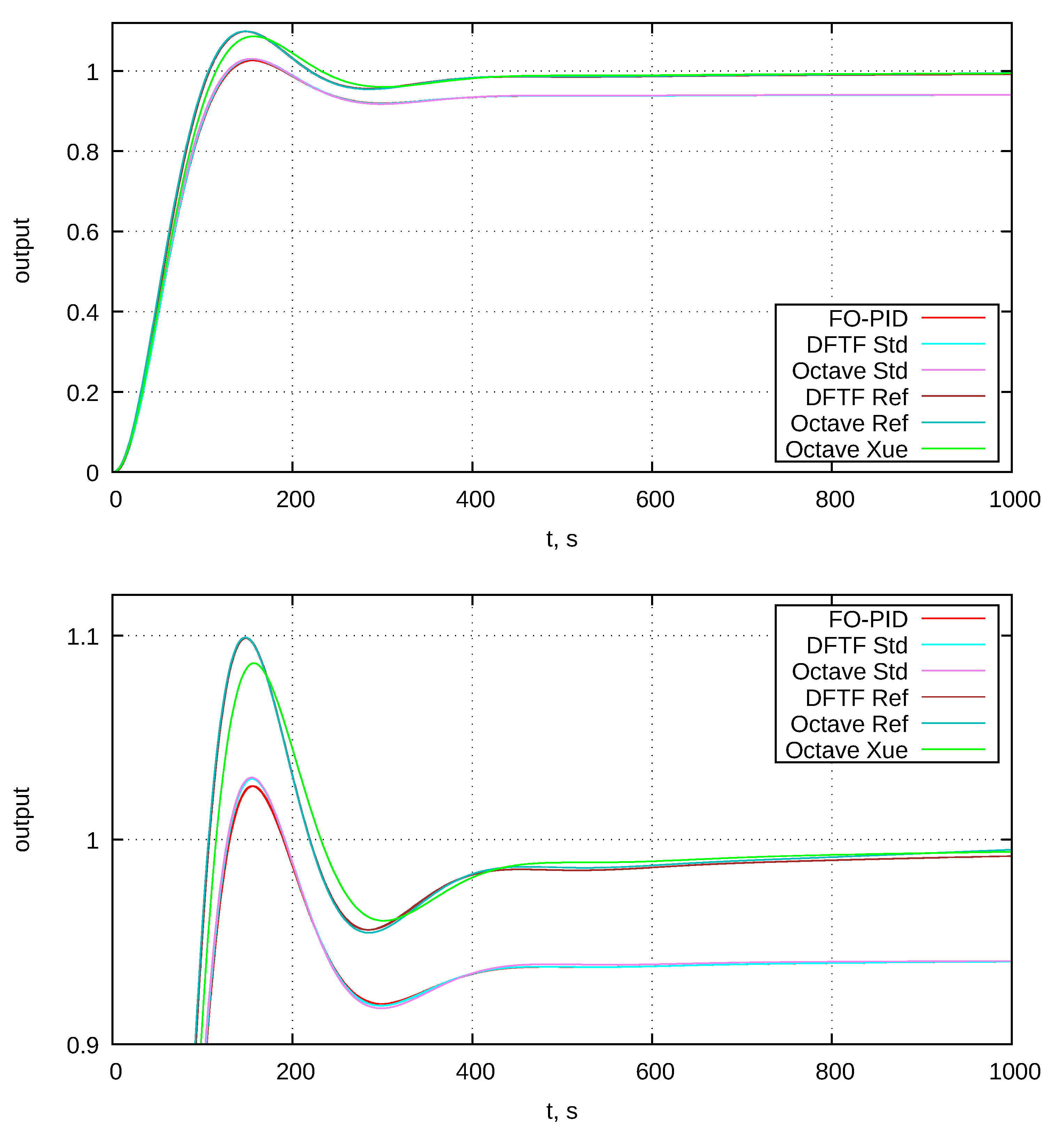
5.4. Closed-Loop Control System

To validate the influence of the selected model on the answer of FO control system, we take the same example as in our previous works [22,68]. It is a real case described elsewhere [24]. The plant is a motor-generator system approximated by second-order inertia with a small delay, described by:

$$G_p\left(s\right)=\frac{0.63606}{(42.77s+1)(7.45s+1)}{e}^{-0.61s}.$$

(24)

The controller is PI${}^{\lambda }$D${}^{\mu }$ type with the transfer function of

$$G_c\left(s\right)=k\left(1+\frac{1}{T_{\mathrm{i}}{s}^{\lambda }}+T_{\mathrm{d}}{s}^{\mu }\right).$$

(25)

Parameters of the controller are cited after [24] and gathered in

Table 5. Tuning parameters of the PI${}^{\lambda }$D${}^{\mu }$ controllers used in simulations—taken from [24].

k	${\mathit{T}}_{\mathbf{i}}$	${\mathit{T}}_{\mathbf{d}}$	$\mathit{\lambda }$	$\mathit{\mu }$
$0.133$	$2.5$	$0.76$	$0.89$	$0.44$

.

The MATLAB Simulink diagram consists of the FO-PID block realizing the PI${}^{\lambda }$D${}^{\mu }$ function. We compare the response of the system containing this block with the system with PI${}^{\lambda }$D${}^{\mu }$ controller built from Discrete Fractional Transducer Functions (DFTFs)—see Figure 8. The DFTF allows switching between the refined and standard variant of the Oustaloup filter approximation—see Figure 9. Additionally, we calculate the response of the system using our own procedure run in Octave which implements the three variants of the filter.

Figure 10 presents the responses of the control system. We observe very similar trajectory calculated using FO-PID, DFTF with unselected refined variant, and our procedure with the standard variant of the Oustaloup filter approximation. It proves that our procedure does not consist of defects and that the FO-PID block uses the standard filter. The slight difference shown at about 150 s comes probably from different sampling period which is unselectable in the FO-PID block. The responses calculated using Simulink and Octave are practically the same. Xue’s variant of the filter has the trajectory similar to that of refined filter but differs slightly. The fundamental conclusion led from the observation is that the shape of the response is dependent on the chosen model. The previous work [22] proves that also parameters used in the approximation influence the shape. It means that the parameters of the FO model obtained by best-fitting to experimental results are biased by choosing the approximation model and its parameters. In the same way, models of sensors, chemical, or physical systems, described by FO differential equations, will have parameters whose values are dependent on the chosen model approximating FO differentiation.

6. Conclusions

The article emphasizes the very often diminished problem, that numerical values calculated by fractional-order differential equations are not accurate. The beginning example shows that the steady-state value of an FO dynamic system may differ from expected value making a bias. The bias is dependent on the selected approximation method and its parameters. It is possible in the frequency domain to calculate the Nyquist plots accurately. It allows for a calculation of the amplitude and phase errors which arose by applying the approximations. Comparison of three variants of the Oustaloup filter approximation evidenced that Xue’s approach, Equation (7), is the most accurate. The impact of the order of the approximation filter (if it is high enough, greater than four for the studied example) on the Nyquist plot is lower than of the approximation model. It is impossible to calculate a reference (accurate) time response of an FO system, so errors cannot be provided in. Plotted unit step responses show different trajectories dependent mostly on models approximating the FO derivative, less on the order of the approximation. Similarly, a control system with a PI${}^{\lambda }$D${}^{\mu }$ controller gives time responses dependent on the applied model. For models of systems, including sensors, providing parameters related to FO differential equation are poor without explicitly specified the approximation method. The more flexible trajectory of the time response of the FO system is paid for by an increase in computational complexity, additional errors (biases) arisen from the selected approximation method and the influence of the method used on parameters of the model.

This work studied only three variants of the Oustaloup filter approximating the fractional derivative. Other known approaches dealing with fractional calculus may introduce similar inaccuracies which should be taken into consideration especially in implementations requiring high precision.

References

1. Barbosa, R.S.; Machado, J.A.T. Implementation of discrete-time fractional-order controllers based on LS approximations. Acta Polytech. Hung. 2006, 3, 5–22. [Google Scholar]
2. Vinagre, B.M.; Chen, Y.Q.; Petráš, I. Two direct Tustin discretization methods for fractional-order differentiator/integrator. J. Frankl. Inst. 2003, 340, 349–362. [Google Scholar] [CrossRef]
3. David, S.A.; Linares, J.L.; Pallone, E.M.J.A. Fractional order calculus: Historical apologia, basic concepts and some applications. Rev. Bras. Ensino Física 2011, 33, 4302. [Google Scholar] [CrossRef]
4. Mandelbrot, B.B. The Fractal Geometry of Nature, 1st ed.; W. H. Freeman and Company: San Francisco, CA, USA, 1982. [Google Scholar]
5. Lu, Y.; Tang, Y.; Zhang, X.; Wang, S. Parameter identification of fractional order systems with nonzero initial conditions based on block pulse functions. Measurement 2020, 158, 107684. [Google Scholar] [CrossRef]
6. Tustin, A.; Allanson, J.T.; Layton, J.M.; Jakeways, R.J. The design of systems for automatic control of the position of massive objects. Proc. IEE Part C Monogr. 1958, 105, 1. [Google Scholar] [CrossRef]
7. Manage, S. The Non-integer Integral and its Application to Control Systemes. J. Inst. Electr. Eng. Jpn. 1960, 80, 589–597. [Google Scholar] [CrossRef]
8. Dogruer, T.; Tan, N. Design of PI Controller using Optimization Method in Fractional Order Control Systems. IFAC Papers OnLine 2018, 51, 841–846. [Google Scholar] [CrossRef]
9. Podlubny, I. Fractional Differential Equations; Academic Press: San Diego, CA, USA, 1998. [Google Scholar]
10. Oziablo, P.; Mozyrska, D.; Wyrwas, M. Discrete-Time Fractional, Variable-Order PID Controller for a Plant with Delay. Entropy 2020, 22, 771. [Google Scholar] [CrossRef]
11. Yaghi, M.; Efe, M.O. H2/H-Neural-Based FOPID Controller Applied for Radar-Guided Missile. IEEE Trans. Ind. Electron. 2020, 67, 4806–4814. [Google Scholar] [CrossRef]
12. Wang, N.; Wang, J.; Li, Z.; Tang, X.; Hou, D. Fractional-Order PID Control Strategy on Hydraulic-Loading System of Typical Electromechanical Platform. Sensors 2018, 18, 3024. [Google Scholar] [CrossRef] [Green Version]
13. Acharya, D.S.; Mishra, S.K. A multi-agent based symbiotic organisms search algorithm for tuning fractional order PID controller. Measurement 2020, 155, 107559. [Google Scholar] [CrossRef]
14. Dziedzic, K.; Oprzędkiewicz, K. The Quickly Adjustable Digital FOPID Controller. In Advances in Intelligent Systems and Computing; Springer Nature Switzerland AG: Cham, Switzerland, 2020; pp. 847–856. [Google Scholar] [CrossRef]
15. Ayas, M.S.; Sahin, E. FOPID controller with fractional filter for an automatic voltage regulator. Comput. Electr. Eng. 2020, 106895. [Google Scholar] [CrossRef]
16. Pradhan, R.; Majhi, S.K.; Pradhan, J.K.; Pati, B.B. Optimal fractional order PID controller design using Ant Lion Optimizer. Ain Shams Eng. J. 2020, 11, 281–291. [Google Scholar] [CrossRef]
17. Asgharnia, A.; Jamali, A.; Shahnazi, R.; Maheri, A. Load mitigation of a class of 5-MW wind turbine with RBF neural network based fractional-order PID controller. ISA Trans. 2020, 96, 272–286. [Google Scholar] [CrossRef]
18. Radwan, A.G.; Emira, A.A.; AbdelAty, A.M.; Azar, A.T. Modeling and analysis of fractional order DC-DC converter. ISA Trans. 2018, 82, 184–199. [Google Scholar] [CrossRef]
19. Yang, Z.Z.; Zhou, J.L. An Improved Design for the IIR-Type Digital Fractional Order Differential Filter. In Proceedings of the 2008 International Seminar on Future BioMedical Information Engineering, Wuhan, China, 18 December 2008. [Google Scholar] [CrossRef]
20. Zhang, C.; Zhu, Z.; Zhu, S.; He, Z.; Zhu, D.; Liu, J.; Meng, S. Nonlinear Creep Damage Constitutive Model of Concrete Based on Fractional Calculus Theory. Materials 2019, 12, 1505. [Google Scholar] [CrossRef] [Green Version]
21. Magin, R.L. Fractional calculus models of complex dynamics in biological tissues. Comput. Math. Appl. 2010, 59, 1586–1593. [Google Scholar] [CrossRef] [Green Version]
22. Wiora, J.; Wiora, A. Inaccuracies Revealed During the Analysis of Propagation of Measurement Uncertainty Through a Closed-Loop Fractional-Order Control System. In Lecture Notes in Electrical Engineering; Springer Nature Switzerland AG: Cham, Switzerland, 2019; pp. 213–226. [Google Scholar] [CrossRef]
23. Macias, M.; Sierociuk, D. Modeling of electrical drive system with flexible shaft based on fractional calculus. In Proceedings of the 14th International Carpathian Control Conference (ICCC), Rytro, Poland, 26–29 May 2013. [Google Scholar] [CrossRef]
24. Viola, J.; Angel, L.; Sebastian, J.M. Design and robust performance evaluation of a fractional order PID controller applied to a DC motor. IEEE/CAA J. Autom. Sin. 2017, 4, 304–314. [Google Scholar] [CrossRef]
25. Kumar, S.; Ghosh, A. Identification of fractional order model for a voltammetric E-tongue system. Measurement 2020, 150, 107064. [Google Scholar] [CrossRef]
26. Freeborn, T.J.; Maundy, B.; Elwakil, A.S. Fractional-order models of supercapacitors, batteries and fuel cells: A survey. Mater. Renew. Sustain. Energy 2015, 4. [Google Scholar] [CrossRef] [Green Version]
27. Zou, C.; Zhang, L.; Hu, X.; Wang, Z.; Wik, T.; Pecht, M. A review of fractional-order techniques applied to lithium-ion batteries, lead-acid batteries, and supercapacitors. J. Power Sources 2018, 390, 286–296. [Google Scholar] [CrossRef] [Green Version]
28. Lenzi, E.K.; Ribeiro, H.V.; Zola, R.S.; Evangelista, L.R. Fractional Calculus in Electrical Impedance Spectroscopy: Poisson–Nernst–Planck model and Extensions. Int. J. Electrochem. Sci. 2017, 11677–11691. [Google Scholar] [CrossRef]
29. Hu, M.; Li, Y.; Li, S.; Fu, C.; Qin, D.; Li, Z. Lithium-ion battery modeling and parameter identification based on fractional theory. Energy 2018, 165, 153–163. [Google Scholar] [CrossRef]
30. Zou, C.; Hu, X.; Dey, S.; Zhang, L.; Tang, X. Nonlinear Fractional-Order Estimator with Guaranteed Robustness and Stability for Lithium-Ion Batteries. IEEE Trans. Ind. Electron. 2017, 1. [Google Scholar] [CrossRef]
31. Lu, X.; Li, H.; Chen, N. An indicator for the electrode aging of lithium-ion batteries using a fractional variable order model. Electrochim. Acta 2019, 299, 378–387. [Google Scholar] [CrossRef]
32. Allagui, A.; Freeborn, T.J.; Elwakil, A.S.; Fouda, M.E.; Maundy, B.J.; Radwan, A.G.; Said, Z.; Abdelkareem, M.A. Review of fractional-order electrical characterization of supercapacitors. J. Power Sources 2018, 400, 457–467. [Google Scholar] [CrossRef]
33. Krishnan, G.; Das, S.; Agarwal, V. An Online Identification Algorithm to Determine the Parameters of the Fractional-Order Model of a Supercapacitor. IEEE Trans. Ind. Appl. 2020, 56, 763–770. [Google Scholar] [CrossRef]
34. Wang, Y.; Gao, G.; Li, X.; Chen, Z. A fractional-order model-based state estimation approach for lithium-ion battery and ultra-capacitor hybrid power source system considering load trajectory. J. Power Sources 2020, 449, 227543. [Google Scholar] [CrossRef]
35. Kumar, S.; Ghosh, A. An Improved Fractional-Order Circuit Model for Voltammetric Taste Sensor System With Infused Tea as Analyte. IEEE Sens. J. 2020, 20, 7792–7800. [Google Scholar] [CrossRef]
36. Alimisis, V.; Gourdouparis, M.; Dimas, C.; Sotiriadis, P.P. Implementation of Fractional-order Model of Nickel-Cadmium Cell using Current Feedback Operational Amplifiers. In Proceedings of the 2020 European Conference on Circuit Theory and Design (ECCTD), Sofia, Bulgaria, 7–10 September 2020. [Google Scholar] [CrossRef]
37. Sarathi, V.P.; Uma, G.; Umapathy, M. Realization of Fractional order Inductive Transducer. IEEE Sens. J. 2018, 1. [Google Scholar] [CrossRef]
38. Tian, A.; Zhao, J.; Xiong, H.; Gan, S.; Fu, C. Application of Fractional Differential Calculation in Pretreatment of Saline Soil Hyperspectral Reflectance Data. J. Sens. 2018, 2018, 1–12. [Google Scholar] [CrossRef]
39. Gerolymatou, E.; Vardoulakis, I.; Hilfer, R. Modelling infiltration by means of a nonlinear fractional diffusion model. J. Phys. D: Appl. Phys. 2006, 39, 4104–4110. [Google Scholar] [CrossRef] [Green Version]
40. Agrawal, N.; Kumar, A.; Bajaj, V.; Singh, G.K. Design of Bandpass and Bandstop Infinite Impulse Response Filters Using Fractional Derivative. IEEE Trans. Ind. Electron. 2019, 66, 1285–1295. [Google Scholar] [CrossRef]
41. Prommee, P.; Pienpichayapong, P.; Manositthichai, N.; Wongprommoon, N. OTA-based tunable fractional-order devices for biomedical engineering. AEU Int. J. Electron. Commun. 2021, 128, 153520. [Google Scholar] [CrossRef]
42. Kawala-Janik, A.; Zolubak, M.; Bauer, W.; Nazimek, B.; Sobolewski, T.; Martinek, R.; Sowa, M.; Pelc, M. Implementation of Non-Integer Order Filtering for the Purpose of Disparities Detection in Beta Frequencies—A Pilot Study. In Proceedings of the 2018 23rd International Conference on Methods & Models in Automation & Robotics (MMAR), Międzyzdroje, Poland, 27–30 August 2018. [Google Scholar] [CrossRef]
43. Alimisis, V.; Dimas, C.; Pappas, G.; Sotiriadis, P.P. Analog Realization of Fractional-Order Skin-Electrode Model for Tetrapolar Bio-Impedance Measurements. Technologies 2020, 8, 61. [Google Scholar] [CrossRef]
44. Miljković, N.; Popović, N.; Djordjević, O.; Konstantinović, L.; Šekara, T.B. ECG artifact cancellation in surface EMG signals by fractional order calculus application. Comput. Methods Programs Biomed. 2017, 140, 259–264. [Google Scholar] [CrossRef] [PubMed]
45. Ren, H.; Yin, A.; Zhang, Q. Vibration signal denoising using partial differential equations of arbitrary order. Measurement 2019, 148, 106917. [Google Scholar] [CrossRef]
46. Wu, C.; Yang, J.; Huang, D.; Liu, H.; Hu, E. Weak signal enhancement by fractional-order system resonance and its application in bearing fault diagnosis. Meas. Sci. Technol. 2019, 30, 035004. [Google Scholar] [CrossRef]
47. Tolba, M.F.; AbdelAty, A.M.; Soliman, N.S.; Said, L.A.; Madian, A.H.; Azar, A.T.; Radwan, A.G. FPGA implementation of two fractional order chaotic systems. AEU Int. J. Electron. Commun. 2017, 78, 162–172. [Google Scholar] [CrossRef]
48. Boukamp, B.A. Derivation of a Distribution Function of Relaxation Times for the (fractal) Finite Length Warburg. Electrochim. Acta 2017, 252, 154–163. [Google Scholar] [CrossRef]
49. Jakubiec, B. Fuzzy logic controller for robot manipulator control system. In Proceedings of the 2018 Applications of Electromagnetics in Modern Techniques and Medicine (PTZE), Racławice, Poland, 9–12 September 2018. [Google Scholar] [CrossRef]
50. Tepljakov, A.; Petlenkov, E.; Belikov, J. FOMCOM: A MATLAB toolbox for fractional-order system identification and control. Int. J. Microelectron. Comput. Sci. 2011, 2, 51–62. [Google Scholar]
51. Xue, D.; FOTF Toolbox. MATLAB Central File Exchange. Available online: https://www.mathworks.com/matlabcentral/fileexchange/60874-fotf-toolbox (accessed on 12 October 2020).
52. Ashwin Pajankar, S.C. GNU Octave by Example; Apress: New York City, NY, USA, 2020. [Google Scholar]
53. Chen, Y.; Petras, I.; Xue, D. Fractional order control-A tutorial. In Proceedings of the 2009 American Control Conference, St. Louis, MO, USA, 10–12 June 2009. [Google Scholar] [CrossRef]
54. Caputo, M.C.; Torres, D.F. Duality for the left and right fractional derivatives. Signal Process. 2015, 107, 265–271. [Google Scholar] [CrossRef] [Green Version]
55. Ortigueira, M.D. Fractional Calculus for Scientists and Engineers; Springer Science+Business Media B.V.: Dordrecht, The Netherlands, 2011. [Google Scholar]
56. Kilbas, A.A.; Srivastava, H.M.; Trujillo, J.J. Theory and Applications of Fractional Differential Equations; Elsevier: Amsterdam, The Netherlands, 2006. [Google Scholar]
57. Vinagre, B.M.; Podlubny, I.; Hernandez, A.; Feliu, V. Some approximations of fractional order operators used in control theory and applications. Fract. Calc. Appl. Anal. 2000, 3, 231–248. [Google Scholar]
58. Atherton, D.P.; Tan, N.; Yüce, A. Methods for computing the time response of fractional-order systems. IET Control Theory Appl. 2015, 9, 817–830. [Google Scholar] [CrossRef]
59. Ionescu, C.; Machado, J.T.; Keyser, R.D. Fractional-order impulse response of the respiratory system. Comput. Math. Appl. 2011, 62, 845–854. [Google Scholar] [CrossRef]
60. Baranowski, J.; Bauer, W.; Zagorowska, M.; Dziwinski, T.; Piatek, P. Time-domain Oustaloup approximation. In Proceedings of the 2015 20th International Conference on Methods and Models in Automation and Robotics (MMAR), Międzyzdroje, Poland, 24–27 August 2015. [Google Scholar] [CrossRef]
61. Xue, D.; Zhao, C.; Chen, Y. A Modified Approximation Method of Fractional Order System. In Proceedings of the 2006 International Conference on Mechatronics and Automation, Luoyang, China, 25–28 June 2006. [Google Scholar] [CrossRef]
62. Xue, D.; Chen, Y.; Atherton, D.P. Linear Feedback Control: Analysis and Design with MATLAB; SIAM: Philadelphia, PA, USA, 2007. [Google Scholar]
63. Krajewski, W.; Viaro, U. A method for the integer-order approximation of fractional-order systems. J. Frankl. Inst. 2014, 351, 555–564. [Google Scholar] [CrossRef]
64. Gluskin, E. Let us teach this generalization of the final-value theorem. Eur. J. Phys. 2003, 24, 591–597. [Google Scholar] [CrossRef]
65. Bialkowski, S.E. Real-time digital filters: finite impulse response filters. Anal. Chem. 1988, 60, 355A–361A. [Google Scholar] [CrossRef]
66. Reade, J.B. Calculus with Complex Numbers; Taylor & Francis: London, UK, 2003. [Google Scholar]
67. Oprzędkiewicz, K. Discrete Transfer Function Models for Non Integer Order Inertial System. In Advances in Intelligent Systems and Computing; Springer International Publishing: Cham, Switzerland, 2018; pp. 14–25. [Google Scholar] [CrossRef]
68. Wiora, J.; Wiora, A. Measurement Uncertainty Evaluation of Results Provided by Transducers Working in Control Loops. In Proceedings of the 2018 23rd International Conference on Methods & Models in Automation & Robotics (MMAR), Międzyzdroje, Poland, 27–30 August 2018. [Google Scholar] [CrossRef]
Figure 1. Nyquist plot of FO inertia with α = 0.9 approximated with refined Oustaloup filter.
Symmetry 12 01898 g001
Figure 2. Nyquist plot of FO inertia with α = 0.9 approximated with Xue’s variant of Oustaloup filter.
Symmetry 12 01898 g002
Figure 3. Nyquist plot of FO inertia with α = 0.6 approximated with the Oustaloup filter.
Symmetry 12 01898 g003
Figure 4. Nyquist plot of FO inertia with α = 0.6 approximated with the refined Oustaloup filter.
Symmetry 12 01898 g004
Figure 5. Nyquist plot of FO inertia with α = 0.6 approximated with Xue’s variant of the Oustaloup filter.
Symmetry 12 01898 g005
Figure 6. Unit step responses of FO inertia with α = 0.9 approximated with different Oustaloup filters. The filters are described by: Std—Equation (5), Ref—Equation (6), Xue—Equation (7). N F is the filter order.
Symmetry 12 01898 g006
Figure 7. Unit step responses of FO inertia with α = 0.6 approximated with different Oustaloup filters. The filters are described by: Std—Equation (5), Ref—Equation (6), Xue—Equation (7). N F is the filter order.
Symmetry 12 01898 g007
Figure 8. Part of Simulink diagram used during simulations. The upper part presents the FO-PID block. The lower part presents the FO controller build from Discrete Fractional Transducer Functions (DFTFs).
Symmetry 12 01898 g008
Figure 9. Simulink dialog boxes showing available parameters. (a) FO-PID allows imputing parameters of PID controller calculated using standard Oustaloup approximation. (b) Discrete Fractional Transfer Functions allow imputing FO poles and zeros, as well as the choice between the standard and refined variant of Oustaloup approximation, additionally, discretization parameters: method, critical frequency, and sampling time.
Symmetry 12 01898 g009
Figure 10. Unit step responses of the closed-loop control system with PI λ D μ . The system consists of the PI λ D μ controller implemented as: FO-PID—the Simulink the FO-PID block, DFTF Std—the Simulink circuit with the DFTF blocks with unselected refined filter, Octave Std—the Octave procedure with the standard Oustaloup filter approximation, DFTF Ref—the Simulink circuit with the DFTF blocks with selected refined filter, Octave Ref—the Octave procedure with the refined Oustaloup filter approximation, Octave Xue—the Octave procedure with Xue’s variant of Oustaloup filter approximation.
Symmetry 12 01898 g010