Slashed Lomax Distribution and Regression Model

Abstract

In this article, the slashed Lomax distribution is introduced, which is an asymmetric distribution and can be used for fitting thick-tailed datasets. Various properties are explored, such as the density function, hazard rate function, Renyi entropy, r-th moments, and the coefficients of the skewness and kurtosis. Some useful characterizations of this distribution are obtained. Furthermore, we study a slashed Lomax regression model and the expectation conditional maximization (ECM) algorithm to estimate the model parameters. Simulation studies are conducted to evaluate the performances of the proposed method. Finally, two sets of data are applied to verify the importance of the slashed Lomax distribution.

1. Introduction

The Lomax distribution, which was introduced by Lomax [1], has been regarded as the mixed distribution of the exponential distribution and gamma distribution. It has a heavy-tailed probability distribution, often used in business, economics, and actuarial modeling. Let X be a non-negative random variable with a Lomax distribution, then its probability density function (pdf) is given by,

$$f\left(x;\alpha ,\beta \right)=\frac{\alpha {\beta }^{\alpha }}{{\left(\beta +x\right)}^{\alpha +1}},$$

where $\alpha >0$ and $\beta >0$, and it is denoted by $X\sim Lomax\left(\alpha ,\beta \right)$. The Lomax distribution contains the monotone decreasing failure rate and the monotone increasing failure rate, which have been regarded as a quantitative life distribution. It has been applied broadly in practical production and real life. For example: Myhre and Saunders [2] applied the Lomax distribution to right censored data; Balakrishnan and Ahsanullah [3] discussed some important statistical properties of the Lomax distribution; Childs et al. [4] studied the properties of right-truncated Lomax distributions and discussed some practical applications; and Howlader and Hossain [5] considered estimating the survival function of the Lomax distribution with the Bayesian method.

The slashed distribution was proposed to model the bell shaped data with a heavier tail, by Rogers and Tukey [6], which is thicker than the tail of the normal distribution and is itself a symmetric distribution. It has a stochastic representation as $Z{U}^{-\frac{1}{q}}$, where $q>0$, $Z\sim N\left(0,1\right)$ is independent of $U\sim U\left(0,1\right)$, and is called the canonical slashed distribution when $q=1$. After that, statisticians have done in-depth research on and promoted this model; see Wang and Genton [7], Gomez et al. [8], Arslan and Genc [9], Reyes et al. [10], and Tian et al. [11,12]. Recently, there has been a new extension of the slashed distribution: Gui [13] introduced a three-parameter extension model called the Lindley slashed distribution; Iriarte et al. [14,15] proposed the slashed Rayleigh distribution and modified slashed Rayleigh distribution, which have a more flexible kurtosis than the Rayleigh distribution; Reyes et al. [16] discussed the modified slashed Birnbaum–Saunders distribution and concluded that it has greater kurtosis values than the usual BSdistribution. Similar to this methodology, the slashed Lindley–Weibull distribution was introduced by Reyes et al. [17]; the slashed power Lindley distributions was studied by Iriarte et al. [18]; and the modified slashed generalized exponential distribution was introduced by Astorga et al. [19].

Regression models are undoubtedly the most widely used, but the normality assumption of the residual errors is more restrictive. Recently, the error term subject to a more flexible distribution has been studied: Gómez [20] analyzed the regression model of the slashed half-normal distribution; Jamal [21] studied the properties of the Topp–Leone–Weibull Lomax distribution and its regression model; and Hamedani et al. [22] analyzed the regression model of the Burr XII distribution.

Based on the previous research, we propose the slashed Lomax distribution, which has a thicker tail than the Lomax distribution and has more flexibility in kurtosis. Furthermore, the construction of the slashed Lomax distribution makes it possible to estimate the parameters in a variety of ways. Therefore, the proposed new distribution can be used not only for fitting thick-tailed datasets, but also can analyze some phenomena in real life. The rest of the paper is organized as follows. In Section 2, we introduce the slashed Lomax distribution and obtain some of its properties. The ECM algorithm for the parameter estimation and simulation studies is proposed in Section 3. The slashed Lomax regression model is studied in Section 4. Two applications to real data are investigated in Section 5. Some conclusions are offered in Section 6.

2. Slashed Lomax Distribution

In this section, some basic properties of the slashed Lomax distribution are described.

Definition 1.

A random variable Y follows a slashed Lomax distribution, denoted as $Y\sim Slomax\left(\alpha ,\beta ,\lambda \right)$, if it can be represented as:

$$Y=V^{-\frac{1}{2}}X,$$

(1)

where $X\sim Lomax\left(\alpha ,\beta \right)$ and $V\sim beta\left(\lambda ,1\right)$ are independent random variables and $\alpha ,\beta ,\lambda >0$.

Proposition 1.

Let $Y\sim Slomax\left(\alpha ,\beta ,\lambda \right)$, then its pdf can be written as:

$${\displaystyle f_Y\left(y;\alpha ,\beta ,\lambda \right)=\frac{2\lambda \alpha {\beta }^{2\lambda }}{y^{2\lambda +1}}{\int }_0^{\frac{y}{\beta }}\frac{w^{2\lambda }}{{\left(1+w\right)}^{\alpha +1}}dw.}$$

(2)

Proof. 

Using the stochastic representation in Equation (1), we have the joint density function of $(Y,V)$ as:

$$f_{Y,V}\left(y,v\right)=\frac{\lambda \alpha v^{\lambda -\frac{1}{2}}}{\beta {(1+\frac{v^{\frac{1}{2}}y}{\beta })}^{\alpha +1}},$$

and the pdf of Y is obtained by marginalizing the distribution with respect to V. □

Corollary 1.

Let $Y\sim Slomax\left(\alpha ,\beta ,\lambda \right)$.

(i)

For $\frac{y}{\beta }<1$,

$$f_Y\left(y;\alpha ,\beta ,\lambda \right)=\frac{2\lambda \alpha }{\left(2\lambda +1\right)\beta }F\left(\alpha +1,2\lambda +1,2\lambda +2;-\frac{y}{\beta }\right),$$

where ${\displaystyle F\left(\alpha ,\beta ,\gamma ;x\right)=\frac{1}{B\left(\beta ,\gamma -\beta \right)}{\int }_0^1{\left(1-t\right)}^{\gamma -\beta -1}{t}^{\beta -1}{\left(1-xt\right)}^{-\alpha }dt}$ is the hyper geometric function.

(ii)

$2\lambda$ and $\alpha -2\lambda$ are positive integers, and $0<\frac{y}{\beta }<1$,

$$f_Y\left(y;\alpha ,\beta ,\lambda \right)=\frac{2\lambda \alpha }{\left(2\lambda +1\right)\beta }B\left(\frac{y}{\beta };2\lambda +1,\alpha -2\lambda \right),$$

where ${\displaystyle B\left(x,y\right)={\int }_0^{\infty }\frac{t^{x-1}}{{\left(1+t\right)}^{x+y}}dt}$ is the incomplete beta function.

Remark 1.

For $\lambda =1$, $Y\sim Slomax\left(\alpha ,\beta ,\lambda \right)$ is reduced to the canonical slashed Lomax distribution, and the pdf is:

$$f_Y\left(y;\alpha ,\beta ,\lambda \right)={\int }_0^1\frac{\alpha v^{\frac{1}{2}}}{\beta {\left(1+\frac{v^{\frac{1}{2}}y}{\beta }\right)}^{\alpha +1}}dv.$$

For an illustration of the new family of slashed Lomax distributions, we draw the density curves, with different values of $\alpha$, $\beta$, and $\lambda$, as follows. After fixing two of the three parameters, we find that the slashed Lomax distributions have a heavier tail as $\beta$ increases (and the same for $\lambda$, but the opposite for $\alpha$).

Proposition 2.

Let $Y\sim Slomax\left(\alpha ,\beta ,\lambda \right)$.

(i)

The reliability (survival) function of Y is given by:

$$R_Y\left(y\right)=1-2\lambda \alpha {\beta }^{2\lambda }{\int }_0^y\frac{A\left(\frac{u}{\beta };\alpha ,\beta ,\lambda \right)}{u^{2\lambda +1}}du,$$

where ${\displaystyle A\left(\frac{y}{\beta };\alpha ,\beta ,\lambda \right)={\int }_0^{\frac{y}{\beta }}\frac{w^{2\lambda }}{{\left(1+w\right)}^{\alpha +1}}dw}$.

(ii)

The hazard rate function of Y is given by:

$$h_Y\left(y;\alpha ,\beta ,\lambda \right)=\frac{2\lambda \alpha {\beta }^{2\lambda }}{y^{2\lambda +1}}A\left(\frac{y}{\beta };\alpha ,\beta ,\lambda \right){\left(1-2\lambda \alpha {\beta }^{2\lambda }{\int }_0^y\frac{A\left(\frac{u}{\beta };\alpha ,\beta ,\lambda \right)}{u^{2\lambda +1}}du\right)}^{-1}.$$

(iii)

The reversed hazard rate of Y is given by:

$$r_Y\left(y\right)=\frac{f\left(y\right)}{F\left(y\right)}=\frac{A\left(\frac{y}{\beta };\alpha ,\beta ,\lambda \right)}{{\displaystyle y^{2\lambda +1}{\int }_0^y\frac{A\left(\frac{u}{\beta };\alpha ,\beta ,\lambda \right)}{u^{2\lambda +1}}du}}.$$

Figure 1 shows probability density function curve of the slashed Lomax distribution with several different parameters. Figure 2 shows the curves of hazard rate functions under different parameters. It can be seen that the values of the hazard rate function based on $\lambda$, with $\alpha$ and $\beta$ fixed, have small differences as y increases in these figures.

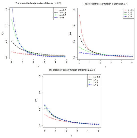
Figure 1. The probability density function plots of Slomax ($\alpha ,\beta ,\lambda$).

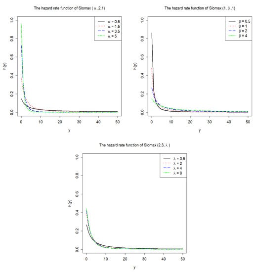
Figure 2. Hazard rate function plots of Slomax ($\alpha ,\beta ,\lambda$).

Next, the Renyi entropy and distributional moments of the slashed Lomax distribution are derived. In addition, the coefficients of skewness and kurtosis are calculated.

Proposition 3.

Let $Y\sim Slomax\left(\alpha ,\beta ,\lambda \right)$; the Renyi entropy of order δ for Y is given by,

$$\begin{array}{c}\hfill R_{\delta }\left(y\right)=\frac{1}{1-\delta }\left[\delta log\left(\frac{\alpha \lambda }{\beta }\right)+log{\int }_0^{\infty }{\left({\int }_0^1\frac{v^{\lambda -\frac{1}{2}}}{{\left(1+\frac{v^{\frac{1}{2}}y}{\beta }\right)}^{\alpha +1}}\right)}^{\delta }dy\right],\end{array}$$

where $\delta >0$ and $\delta \ne 1$.

Proof. 

Renyi entropy is an important diversity index in ecology and statistics, which is defined as ${\displaystyle R_{\delta }\left(y\right)=\frac{1}{1-\delta }log\left[{\int }_0^{\infty }{f\left(y\right)}^{\delta }dy\right]}$. Therefore, we have:

$$\begin{array}{cc}\hfill R_{\delta }\left(y\right)=& \frac{1}{1-\delta }log\left[{\left(\frac{\alpha \lambda }{\beta }\right)}^{\delta }{\int }_0^{\infty }{\left({\int }_0^1\frac{v^{\lambda -\frac{1}{2}}}{{\left(1+\frac{v^{\frac{1}{2}}y}{\beta }\right)}^{\alpha +1}}\right)}^{\delta }dy\right]\hfill \\ \hfill =& \frac{1}{1-\delta }\left[\delta log\left(\frac{\alpha \lambda }{\beta }\right)+log{\int }_0^{\infty }{\left({\int }_0^1\frac{v^{\lambda -\frac{1}{2}}}{{\left(1+\frac{v^{\frac{1}{2}}y}{\beta }\right)}^{\alpha +1}}\right)}^{\delta }dy\right].\hfill \end{array}$$

 □

Proposition 4.

Let $Y\sim$ Slomax$\left(\alpha ,\beta ,\lambda \right)$; the r-th moment of Y, for $r=1,2\cdots$ and $r<2\lambda$, is given by:

$${\mu }_r=\frac{2\lambda \beta \Gamma \left(\alpha -r\right)\Gamma \left(r+1\right)}{(2\lambda -r)\Gamma \left(\alpha \right)},$$

(3)

where $\Gamma (·)$ is the gamma function.

Proof. 

Using Equation (1), we have,

$${\mu }_r=E\left(Y^r\right)=E\left(X^r\right)E\left(V^{-\frac{r}{2}}\right).$$

According to the properties of the beta distribution and the Lomax distribution, we have that ${\displaystyle E\left(V^{-r}\right)=\frac{\lambda }{\lambda -r},}$ for $r<\lambda$, and ${\displaystyle E\left(X^r\right)=\frac{\beta \Gamma \left(\alpha -r\right)\Gamma \left(r+1\right)}{\Gamma \left(\alpha \right)}}$. Thus, the result is obtained. □

Corollary 2.

Let $Y\sim$ Slomax $\left(\alpha ,\beta ,\lambda \right)$; the mean and variance of Y are given by:

$${\displaystyle E\left(Y\right)=\frac{2\lambda \beta }{\left(2\lambda -1\right)\left(\alpha -1\right)},}$$

$$Var\left(Y\right)=\frac{{\left(2\lambda -1\right)}^2\left(\alpha -1\right)}{\lambda \beta \left(2\lambda -2\right)\left(\alpha -2\right)}.$$

Corollary 3.

Let $Y\sim$ Slomax $\left(\alpha ,\beta ,\lambda \right)$; the coefficients of skewness and kurtosis for Y, ${\gamma }_1$ and ${\gamma }_2$, are given by:

$$\begin{array}{cc}\hfill {\gamma }_1=& \frac{{\left(\lambda \beta \right)}^{\frac{5}{2}}{\left(2\lambda -2\right)}^{\frac{1}{2}}{\left(\alpha -2\right)}^{\frac{1}{2}}{\Delta }_1}{{\left(\alpha -1\right)}^{\frac{9}{2}}\left(\alpha -3\right){\left(2\lambda -1\right)}^6\left(2\lambda -3\right)},\hfill \end{array}$$

$$\begin{array}{cc}\hfill {\gamma }_2=& \frac{16{\lambda }^3{\beta }^3\left(2\lambda -2\right)\left(\alpha -2\right){\Delta }_2}{{\left(\alpha -1\right)}^6\left(\alpha -3\right)\left(\alpha -4\right){\left(2\lambda -1\right)}^8\left(2\lambda -3\right)\left(2\lambda -4\right)},\hfill \end{array}$$

where ${\Delta }_1=12{(\alpha -1)}^2{(2\lambda -1)}^3(2\lambda -2)-24\lambda \beta (\alpha -1)(\alpha -3){(2\lambda -1)}^2(2\lambda -3)+16{\beta }^2{\lambda }^2(\alpha -2)(\alpha -3)(2\lambda -2)(2\lambda -3)$ and ${\Delta }_2=3{(\alpha -1)}^3{(2\lambda -1)}^4(2\lambda -2)(2\lambda -3)-3\lambda \beta {(\alpha -1)}^2(\alpha -4){(2\lambda -1)}^3(2\lambda -2)(2\lambda -4)+4{\lambda }^2{\beta }^2(\alpha -1)(\alpha -3)(\alpha -4){(2\lambda -1)}^2(2\lambda -3)(2\lambda -4)-3{\lambda }^3{\beta }^3(\alpha -2)(\alpha -3)(\alpha -4)(2\lambda -2)(2\lambda -3)(2\lambda -4)$.

Proof. 

From Proposition 4, ${\displaystyle {\gamma }_1=\frac{{\mu }_3-3{\mu }_2{\mu }_1+2{\mu }_1^3}{{\left({\mu }_2-{\mu }_1^2\right)}^{\frac{3}{2}}}}$ and ${\displaystyle {\gamma }_2=\frac{{\mu }_4-4{\mu }_1{\mu }_3+6{\mu }^2{\mu }_2-3{\mu }_1^4}{{\left({\mu }_2-{\mu }_1^2\right)}^2}}$; thus, the results are obtained directly. □

In the following propositions, we consider the linear transformation of the slashed Lomax distribution and discuss its scale mixture representation.

Proposition 5.

Let $Y\sim Slomax(\alpha ,\beta ,\lambda )$ and the scalar $a>0$, then $aY\sim Slomax(\alpha ,a\beta ,\lambda )$.

Proof. 

Let $X\sim Lomax(\alpha ,\beta )$, and $a>0$ is a scalar; we have $aX\sim Lomax(\alpha ,a\beta )$. Therefore, the result is obtained by Equation (1). □

Proposition 6.

If $Y|V=v\sim Lomax\left(\alpha ,v^{-\frac{1}{2}}\beta \right)$ and V∼ beta ($\lambda ,1$), then Y∼ Slomax($\alpha ,\beta ,\lambda$).

Proof. 

The result can be obtained by Equation (1) and Proposition 1. □

3. ECM Algorithm for Parameter Estimation

In this section, we consider the maximum likelihood (ML) estimation for the parameters $\mathit{\theta }={\left(\alpha ,\beta ,\lambda \right)}^{\prime }$ of the slashed Lomax distribution. It is well known that the EM algorithm is an important tool for ML estimation when no data or potential variables are observed. The E-step is used to find the expectation of the incomplete data based on the observed values, and the M-step works for the maximization. Usually, the M-step calculation is difficult when the maximum likelihood of the complete data is complex. Meng and Rubin [23] proposed an ECM algorithm that was an extension of the EM algorithm and satisfied all the properties of the EM algorithm. The basic idea of the ECM algorithm is to decompose the M-step of the EM algorithm into k times conditional maximization.

In the following, an ECM algorithm is proposed for obtaining the estimator of $\mathit{\theta }$ from the slashed Lomax distribution. Let $y_1,\cdots ,y_n$ be a random sample from $Slomax\left(\alpha ,\beta ,\lambda \right)$. According to Equation (1), we have,

$$\begin{array}{cc}\hfill & y_i|v_i=v_i\sim Lomax\left(\alpha ,v_i^{-\frac{1}{2}}\beta \right),\hfill \\ \hfill & v_i\sim beta\left(\lambda ,1\right).\hfill \end{array}$$

Let $\mathbf{y}={\left(y_1,...,y_n\right)}^{\prime }$ and $\mathbf{v}={\left(v_1,...,v_n\right)}^{\prime }$ be observed data, then ($y_i,v_i$), $i=1,\cdots ,n$ are the complete dataset. Therefore, the log-likelihood function for the complete data $(y_i,v_i)$, $i=1,\cdots ,n$, is given by:

$$\begin{array}{cc}\hfill l\left(\mathit{\theta }\right)& =nlog\left(\lambda \right)+nlog\left(\alpha \right)-nlog\left(\beta \right)+\left(\alpha +1\right)nlog\left(\beta \right)+\left(\lambda -\frac{1}{2}\right)\sum _{i=1}^{n}log\left(v_i\right)\hfill \\ \hfill & -\left(\alpha +1\right)\sum _{i=1}^{n}log\left(\beta +{v_i}^{\frac{1}{2}}{y}_i\right).\hfill \end{array}$$

E-Step: Compute the conditional expectation of the log-likelihood function, $Q\left(\mathit{\theta },{\widehat{\mathit{\theta }}}^{(k-1)}\right)=E[l\left(\mathit{\theta }\right)|y,{\widehat{\mathit{\theta }}}^{(k-1)}]$, by using the following equation,

$$\begin{array}{cc}\hfill Q\left(\mathit{\theta },{\widehat{\mathit{\theta }}}^{(k-1)}\right)& =nlog\left({\lambda }^{(k-1)}\right)+nlog\left({\alpha }^{(k-1)}\right)+{\alpha }^{(k-1)}nlog\left({\beta }^{(k-1)}\right)\hfill \\ \hfill & +\left({\lambda }^{(k-1)}-\frac{1}{2}\right)\sum _{i=1}^n{\delta }_{1i}^{(k-1)}-\left(\alpha +1\right)\sum _{i=1}^n{\delta }_{2i}^{(k-1)},\hfill \end{array}$$

where ${\delta }_{1i}=E\left[log{v}_i|y_i,\widehat{\mathit{\theta }}\right],{\delta }_{2i}=E\left[log(\beta +v_i^{\frac{1}{2}}{y}_i)|y_i,\widehat{\mathit{\theta }}\right]$.

CM-Steps: Maximize $Q\left(\mathit{\theta },{\widehat{\mathit{\theta }}}^{(k-1)}\right)$ with respect to $\mathit{\theta }$ to obtain ${\left(\widehat{\mathit{\theta }}\right)}^{\left(k\right)}$.

Denote ${\displaystyle W^{(k-1)}={\int }_0^{\frac{y}{{\widehat{\beta }}^{(k-1)}}}\frac{w^{2{\widehat{\lambda }}^{(k-1)}}}{{\left(1+w\right)}^{{\widehat{\alpha }}^{(k-1)}+1}}dw}$; the following equations are obtained for the maximization.

(i)

Set up ${\displaystyle \frac{\partial Q\left(\mathit{\theta },{\widehat{\mathit{\theta }}}^{(k-1)}\right)}{\partial \alpha }=\frac{n}{{\widehat{\alpha }}^{\left(k\right)}}+nlog\left({\widehat{\beta }}^{(k-1)}\right)-\sum _{i=1}^n{\delta }_{2i}^{(k-1)}=0}$, then:

$${\displaystyle {\widehat{\alpha }}^{\left(k\right)}=\frac{n}{{\sum }_{i=1}^n{\delta }_{2i}^{(k-1)}-nlog\left({\widehat{\beta }}^{(k-1)}\right)},}$$

(4)

where ${\displaystyle {\delta }_{2i}^{(k-1)}=\frac{{y_i}^{2{\widehat{\lambda }}^{(k-1)}}+1}{2W^{(k-1)}{\left({\widehat{\beta }}^{(k-1)}\right)}^{2{\widehat{\lambda }}^{(k-1)}+1}}{\int }_0^{1}log\left({\widehat{\beta }}^{(k-1)}+v^{\frac{1}{2}}{y}_i\right)\frac{v^{{\widehat{\lambda }}^{(k-1)}-\frac{1}{2}}}{{(1+{\frac{y_i}{\widehat{\beta }}}^{(k-1)})}^{{\widehat{\alpha }}^{(k-1)}+1}}dv.}$

(ii)

Set up ${\displaystyle \frac{\partial Q\left(\mathit{\theta },{\widehat{\mathit{\theta }}}^{(k-1)}\right)}{\partial \beta }=\frac{{\widehat{\alpha }}^{\left(k\right)}n}{{\widehat{\beta }}^{\left(k\right)}}-({\widehat{\alpha }}^{\left(k\right)}+1)\sum _{i=1}^n{\delta }_{3i}^{(k-1)}=0}$, then:

$${\displaystyle {\widehat{\beta }}^{\left(k\right)}=\frac{n{\widehat{\alpha }}^{\left(k\right)}}{{\displaystyle \left({\widehat{\alpha }}^{\left(k\right)}+1\right)\sum _{i=1}^n{\delta }_{3i}^{(k-1)}}},}$$

(5)

where ${\displaystyle {\delta }_{3i}^{(k-1)}=\frac{{y_i}^{2{\widehat{\lambda }}^{(k-1)}+1}}{2W^{(k-1)}{\left({\widehat{\beta }}^{(k-1)}\right)}^{2{\widehat{\lambda }}^{(k-1)}+1}}{\int }_0^1{\left({\widehat{\beta }}^{(k-1)}+v^{\frac{1}{2}}{y}_i\right)}^{-1}\frac{v^{{\widehat{\lambda }}^{(k-1)}-\frac{1}{2}}}{{(1+\frac{y_i}{{\widehat{\beta }}^{(k-1)}})}^{{\widehat{\alpha }}^{(k-1)}+1}}dv.}$

(iii)

Set up ${\displaystyle \frac{\partial Q\left(\mathit{\theta },{\widehat{\mathit{\theta }}}^{(k-1)}\right)}{\partial \lambda }=\frac{n}{{\widehat{\lambda }}^{\left(k\right)}}+\sum _{i=1}^n{\delta }_{1i}^{(k-1)}=0}$, then:

$${\widehat{\lambda }}^{\left(k\right)}=-\frac{n}{{\sum }_{i=1}^n{\delta }_{1i}^{(k-1)}},$$

(6)

where ${\displaystyle {\delta }_{1i}^{(k-1)}=\frac{{y_i}^{2{\widehat{\lambda }}^{(k-1)}+1}}{2W{\left({\widehat{\beta }}^{(k-1)}\right)}^{2{\widehat{\lambda }}^{(k-1)}+1}}{\int }_0^{1}log\left(v\right)\frac{v^{{\widehat{\lambda }}^{(k-1)}-\frac{1}{2}}}{{\left(1+\frac{y_i}{{\widehat{\beta }}^{(k-1)}}\right)}^{{\widehat{\alpha }}^{(k-1)}+1}}dv.}$

The iterations are repeated until a suitable convergence rule is satisfied, say $||{\widehat{\mathit{\theta }}}^{\left(k\right)}-{\widehat{\mathit{\theta }}}^{(k-1)}||<ϵ$, where $||·||$ is the Euclidean norm and $ϵ$ is sufficiently small.

In the following, we conduct simulation studies to test the efficiency of the estimation procedure discussed above. The random values following the slashed Lomax distribution can be generated by Equation (1). The parameters are set up as: $\mathit{\theta }=$ (2,1,0.5), (2,1,1), (2,1,1.5), (1,0.5,1), (1,1,1), (1,2,1), (0.5,2,2), (2,2,1), (4,2,1). The sample sizes n = 50, 100, and 200. The following procedure is for generating a random number with size n from $Slomax(\alpha ,\beta ,\lambda )$,

• set $\alpha ,\beta ,\lambda$, and n;
• simulate $U\sim Uniform(0,1)$;
• simulate $V\sim beta(\lambda ,1)$;
• compute $Z=\left({(1-U)}^{{}^{-\frac{1}{\alpha }}}-1\right)\beta$;
• compute $Y=V^{{}^{-\frac{1}{2}}}Z$.

For each scenario, we repeat the process $N=1000$ times. The ECM algorithm is applied, and the results are computed using the software R. The procedures are put in the same conditions (same initial values, and $ϵ={10}^{-4}$). The estimators are obtained by applying the nleqslvfunction in Equations (4)–(6). The mean values of the parameters and the corresponding standard deviation (SD) are shown in Table 1. The empirical estimated mean value and SDs based on the 1000 replicates are calculated by:

$$\begin{array}{c}\hfill Mea{n}_n\left(\xi \right)=\frac{1}{N}\sum _{i=1}^n{\widehat{\xi }}_i,\\ \hfill S{D}_n\left(\xi \right)=\sqrt{\frac{1}{N}\sum _{i=1}^N{({\widehat{\xi }}_i-\xi )}^2},\end{array}$$

where $\xi$ is the interesting parameter, $\alpha ,\beta ,\lambda$, respectively.

Table 1. Estimates for parameters $\alpha ,\beta ,\lambda$ of the slashed Lomax distribution.

Sample	$\mathit{\alpha }$	$\mathit{\beta }$	$\mathit{\lambda }$	$\widehat{\mathit{\alpha }}$(SD)	$\widehat{\mathit{\beta }}$(SD)	$\widehat{\mathit{\lambda }}$(SD)
n = 50	2	1	0.5	1.8883 (0.0848)	1.3074 (0.3761)	0.8684 (0.3455)
	2	1	1	1.9468 (0.0509)	1.0003 (0.2849)	1.1409 (0.5941)
	2	1	1.5	1.9620 (0.0439)	0.9147 (0.2761)	1.3130 (0.7770)
	1	0.5	1	0.9431 (0.0640)	0.4590 (0.1624)	1.1234 (0.6727)
	1	1	1	0.9334 (0.0660)	0.8869 (0.3077)	1.0288 (0.5105)
	1	2	1	0.9305 (0.0676)	1.7732 (0.6035)	0.9922 (0.4897)
	0.5	2	1	0.4480 (0.0408)	1.6718 (0.6684)	0.9473 (0.3461)
	2	2	1	1.9607 (0.0403)	1.9989 (0.5392)	1.1505 (0.6040)
	4	2	1	4.0289 (0.0886)	1.9676 (0.5494)	1.0652 (0.3331)
n = 100	2	1	0.5	1.8869 (0.5755)	1.3423 (0.2870)	0.7882 (0.1667)
	2	1	1	1.9626 (0.4163)	1.0579 (0.2244)	1.2117 (0.5973)
	2	1	1.5	1.9745 (0.0328)	0.9262 (0.1931)	1.4674 (0.6219)
	1	0.5	1	0.9431 (0.0489)	0.4598 (0.1270)	1.1133 (0.6548)
	1	1	1	0.9556 (0.0464)	0.9610 (0.2665)	1.1394 (0.5322)
	1	2	1	0.9572 (0.0447)	1.9481 (0.5402)	1.1264 (0.5208)
	0.5	2	1	0.4677 (0.0304)	1.8369 (0.5869)	1.0834 (0.4289)
	2	2	1	1.9673 (0.3313)	2.0052 (0.4470)	1.1695 (0.5673)
	4	2	1	3.9852 (0.0452)	2.1742 (0.4372)	1.1036 (0.1969)
n = 200	2	1	0.5	1.8961 (0.0425)	1.3209 (0.1952)	0.7660 (0.0732)
	2	1	1	1.9681 (0.0368)	1.0377 (0.1805)	1.1338 (0.5696)
	2	1	1.5	1.9841 (0.0236)	0.9704 (0.1689)	1.5644 (0.5242)
	1	0.5	1	0.9632 (0.0351)	0.5031 (0.1172)	1.1189 (0.4276)
	1	1	1	0.9651 (0.0353)	0.9893 (0.2253)	1.1067 (0.4699)
	1	2	1	0.9667 (0.0353)	1.9817 (0.4290)	1.1444 (0.4659)
	0.5	2	1	0.4755 (0.0235)	1.9270 (0.4552)	1.1307 (0.4125)
	2	2	1	1.9755 (0.0243)	2.0940 (0.3621)	1.1379 (0.5646)
	4	2	1	4.0136 (0.0758)	1.9683 (0.5087)	1.0997 (0.1847)

From Table 1, it can be seen that as the sample size increases, the mean value of estimators comes closer to the true values, and the SD decreases in all case.

4. Slashed Lomax Regression Model

In this section, we study the slashed Lomax regression model and propose the ECM algorithm to estimate the parameters.

Definition 2.

The slashed Lomax regression model is defined as:

$$y=x^{\prime }\gamma +\epsilon ,$$

where $y\in \Re$, $\gamma \in {\Re }^p$ is a p-dimensional vector of regression parameters, $x=({\mathbf{x}}_{\mathbf{1}},{\mathbf{x}}_{\mathbf{2}},...,{\mathbf{x}}_{\mathbf{n}})$ is a known $p\times n$ matrix, with ${\mathbf{x}}_i\in {\Re }^p$ for $i=1,\cdots ,n$, and $\epsilon \sim Slomax(\alpha ,\beta ,\lambda )$.

According to Equation (2), the density function of y is given by:

$$f\left(y\right)={\int }_0^1\frac{\alpha \lambda {\beta }^{\alpha }{v}^{\lambda -\frac{1}{2}}}{{\left(\beta +(y-x^{\prime }\gamma )v^{\frac{1}{2}}\right)}^{\alpha +1}}dv.$$

Let $\mathbf{y}={(y_1,y_2,...y_n)}^{\prime }$ come from the slashed Lomax regression model with X the given design matrix x. The log-likelihood function of $\delta =(\alpha ,\beta ,\lambda ,\gamma )$ can be written as:

$$l(\delta |\mathbf{y},X)=nlog\left(\lambda \right)+nlog\left(\alpha \right)+\alpha nlog\left(\beta \right)+\sum _{i=1}^{n}logM\left(y_i\right),$$

where ${\displaystyle M\left(y_i\right)={\int }_0^1\frac{v^{\lambda -\frac{1}{2}}}{{\left(\beta +(y_i-{\mathbf{x}}_i\gamma )v^{\frac{1}{2}}\right)}^{\alpha +1}}dv}$.

Now, given $\mathbf{v}=(v_1,...v_n)$, we can get the complete log-likelihood function:

$$l(\delta |\mathbf{y},\mathbf{v})=nlog\left(\alpha \right)+nlog\left(\lambda \right)+\alpha nlog\left(\beta \right)+\left(\lambda -\frac{1}{2}\right)\sum _{i=1}^{n}log\left(v_i\right)-(\alpha +1)\sum _{i=1}^{n}log\left(\beta +(y_i-{\mathbf{x}}_i\gamma )v^{\frac{1}{2}}\right),$$

and the conditional expectation of $l(\delta |\mathbf{y},\mathbf{v})$,

$$\begin{array}{cc}\hfill Q\left(\delta \right)& =E\left[l\left(\delta \right)|\mathbf{y},\widehat{\delta }\right]\hfill \\ \hfill & =nlog\left(\lambda \right)+nlog\left(\alpha \right)+\alpha nlog\left(\beta \right)+\left(\lambda -\frac{1}{2}\right)\sum _{i=1}^n{\delta }_{1i}-(\alpha +1)\sum _{i=1}^n{\delta }_{2i},\hfill \end{array}$$

where ${\delta }_{1i}=E\left[log{v}_i|y_i,\widehat{\delta }\right],{\delta }_{2i}=E\left[log(\beta +v_i^{\frac{1}{2}}(y_i-{\mathbf{x}}_i\gamma ))|y_i,\widehat{\delta }\right]$.

In the following, we illustrate the steps for the ECM algorithm for estimating the parameters in the regression model.

E-step: Given ${\widehat{\delta }}^{\left(k\right)}=\left({\widehat{\alpha }}^{\left(k\right)},{\widehat{\beta }}^{\left(k\right)},{\widehat{\lambda }}^{\left(k\right)},{\widehat{\gamma }}^{\left(k\right)}\right)$, find the expectation of the condition.

CM-step I: ${\widehat{\alpha }}^{\left(k\right)}$ must be updated as:

$${\widehat{\alpha }}^{(k+1)}=\frac{n}{{\sum }_{i=1}^n{\delta }_{2i}-nlog\left({\widehat{\beta }}^{\left(k\right)}\right)}.$$

CM-step $II$: ${\widehat{\beta }}^{\left(k\right)}$ must be updated as:

$${\widehat{\beta }}^{(k+1)}=\frac{{\widehat{\alpha }}^{(k+1)}n}{({\widehat{\alpha }}^{(k+1)}+1){\sum }_{i=1}^n{\delta }_{3i}}.$$

CM-step $III$: ${\widehat{\lambda }}^{\left(k\right)}$ must be updated as:

$${\widehat{\lambda }}^{(k+1)}=-\frac{n}{{\sum }_{i=1}^n{\delta }_{1i}}.$$

CM-step $IV$: ${\widehat{\gamma }}^{\left(k\right)}$ must be updated as:

$${\widehat{\gamma }}^{(k+1)}=\underset{\delta }{argmin}\sum _{i=1}^n{\delta }_{2i}.$$

The iterations are repeated until a suitable convergence rule is satisfied, say $|{\widehat{\delta }}^{(k+1)}-{\widehat{\delta }}^{\left(k\right)}|$ sufficiently small. On the basis of this theory, a simulation experiment is carried out. We take the two-dimensional regression model to carry out the numerical simulation. The value of the parameters for $(\alpha ,\beta ,\lambda )$ are chosen as (2,2,1), (1,1,1), (1,4,0.5),(0.5,3,0.5), and the regression parameters $({\gamma }_1,{\gamma }_2)$ are set to (1,4), (−2,3), and (−3,−5); $x_i\sim N(0,1)$, for $i=1,2$, are uncorrelated. For each scenario, we generate $N=1000$ samples of size n = 50, 100, and 200, respectively. The empirical estimated mean value and SDs for the corresponding parameters based on the 1000 replicates are shown in Table 2, Table 3 and Table 4.

Table 2. Estimates for the parameters of the Slomax regression model (n = 50).

Actual Values					Estimated Values (Standard Deviations)
$\mathit{\alpha }$	$\mathit{\beta }$	$\mathit{\lambda }$	${\mathit{\gamma }}_{\mathbf{1}}$	${\mathit{\gamma }}_{\mathbf{2}}$	$\widehat{\mathit{\alpha }}$	$\widehat{\mathit{\beta }}$	$\widehat{\mathit{\lambda }}$	$\widehat{{\mathit{\gamma }}_{\mathbf{1}}}$	$\widehat{{\mathit{\gamma }}_{\mathbf{2}}}$
2	2	1	1	4	2.3164	2.4001	1.3882	1.0299	3.9981
					(1.0269)	(1.0390)	(0.5322)	(0.4223)	(0.4285)
1	1	1	1	4	1.0578	1.1937	1.1643	0.9445	4.0047
					(0.3028)	(0.6507)	(0.1921)	(0.4653)	(0.4501)
1	4	0.5	1	4	0.8551	5.3615	1.1127	0.8441	3.9263
					(0.2407)	(3.3273)	(0.1690)	(1.9800)	(2.2611)
0.5	3	0.5	1	4	0.4843	4.6278	1.0762	0.8408	3.3788
					0.0983	2.9716	0.1368	3.1968	2.2944
2	2	1	−2	3	2.1730	2.3055	1.2889	−2.0105	2.9500
					(0.7806)	(0.9017)	(0.3916)	(0.3225)	(0.3497)
1	1	1	−2	3	1.0584	1.2141	1.1524	−1.9542	2.9697
					(0.3037)	(0.6631)	(0.1387)	(0.3959)	(0.4510)
1	4	0.5	−2	3	0.8338	5.2690	1.1026	−1.9339	2.5350
					(0.2292)	(2.7569)	(0.1260)	(2.5031)	(2.5080)
0.5	3	0.5	−2	3	0.7387	3.2542	0.5982	−1.8997	2.7328
					(0.3441)	(0.5349)	(0.2066)	(0.3553)	(1.4824)
2	2	1	−3	−5	2.2537	2.3481	1.1121	−3.2708	−5.1619
					(0.3472)	(0.3213)	(0.2769)	(0.7314)	(0.5327)
1	1	1	−3	−5	1.0410	1.1262	1.0871	−2.8100	−4.9051
					(0.4803)	(0.3203)	(0.1356)	(0.3583)	(0.3044)
1	4	0.5	−3	−5	0.7334	3.2508	0.3213	−2.5547	−4.3723
					(0.3510)	(1.4735)	(0.3225)	(1.6271)	(1.5240)
0.5	3	0.5	−3	−5	0.4287	2.8513	0.8711	−3.4246	−4.7502
					(0.1308)	(0.2210)	(0.0805)	(1.3251)	(1.1469)

Table 3. Estimates for the parameters of the Slomax regression model (n = 100).

Actual Values					Estimated Values (SD)
$\mathit{\alpha }$	$\mathit{\beta }$	$\mathit{\lambda }$	${\mathit{\gamma }}_{\mathbf{1}}$	${\mathit{\gamma }}_{\mathbf{2}}$	$\widehat{\mathit{\alpha }}$	$\widehat{\mathit{\beta }}$	$\widehat{\mathit{\lambda }}$	$\widehat{{\mathit{\gamma }}_{\mathbf{1}}}$	$\widehat{{\mathit{\gamma }}_{\mathbf{2}}}$
2	2	1	1	4	1.9919	2.1269	1.2682	0.9906	4.0009
					(0.5305)	(0.4709)	(0.2391)	(0.2311)	(0.1808)
1	1	1	1	4	1.0571	1.1489	1.1473	1.0213	4.0196
					(0.2517)	(0.4530)	(0.1452)	(0.2380)	(0.2790)
1	4	0.5	1	4	1.1583	5.0987	1.0734	0.8992	3.9050
					(0.2011)	(2.4680)	(0.1343)	(1.5287)	(1.7334)
0.5	3	0.5	1	4	0.4639	4.1823	1.0946	1.1263	3.7404
					(0.0775)	(1.6672)	(0.1658)	(1.4425)	(1.3554)
2	2	1	−2	3	2.0466	2.1632	1.2692	−1.9791	3.0303
					(0.5222)	(0.4559)	(0.2689)	(0.1964)	(0.2036)
1	1	1	−2	3	1.0346	1.1397	1.1739	−2.0267	2.9309
					(0.2461)	(0.5273)	(0.1933)	(0.2701)	(0.2840)
1	4	0.5	−2	3	0.8323	5.0506	1.0024	−1.9508	2.5885
					(0.1907)	(2.0433)	(0.1102)	(1.5322)	(1.4601)
0.5	3	0.5	−2	3	0.7210	(3.1815	0.5733	−1.9463	2.7575)
					(0.3066)	(0.4831)	(0.2032)	(0.3026)	(0.8780)
2	2	1	−3	−5	2.2334	2.2087	1.0897	−2.8324	−5.1021
					(0.2031)	(0.1894)	(0.2003)	(0.5485)	(0.4097)
1	1	1	−3	−5	1.0327	1.1892	0.9358	−2.9350	−5.1317
					(0.2566)	(0.2387)	(0.1348)	(0.3369)	(0.2447)
1	4	0.5	−3	−5	0.2513	3.7044	0.4024	−2.7307	−5.2522
					(0.3310)	(0.8761)	(0.2550)	(0.5103)	(0.7322)
0.5	3	0.5	−3	−5	0.4553	2.9032	0.5041	−3.3221	−4.8077
					(0.1003)	(0.1757)	(0.0533)	(0.8258)	(0.6045)

Table 4. Estimates for the parameters of the Slomax regression model (n = 300).

Actual Values					Estimated Values (SD)
$\mathit{\alpha }$	$\mathit{\beta }$	$\mathit{\lambda }$	${\mathit{\gamma }}_{\mathbf{1}}$	${\mathit{\gamma }}_{\mathbf{2}}$	$\widehat{\mathit{\alpha }}$	$\widehat{\mathit{\beta }}$	$\widehat{\mathit{\lambda }}$	$\widehat{{\mathit{\gamma }}_{\mathbf{1}}}$	$\widehat{{\mathit{\gamma }}_{\mathbf{2}}}$
2	2	1	1	4	1.8919	2.0056	1.2036	1.0105	3.9960
					(0.2624)	(0.2031)	(0.1497)	(0.0966)	(0.0889)
1	1	1	1	4	1.0082	1.0788	1.1737	0.9764	3.9674
					(0.1296)	(0.2563)	(0.1687)	(0.1455)	(0.1293)
1	4	0.5	1	4	1.0858	4.7333	0.8826	0.9455	4.1321
					(0.1582)	(0.9974)	(0.1125)	(0.9275)	(0.7030)
0.5	3	0.5	1	4	0.4870	3.7324	0.8707	1.0973	3.8105
					(0.0532)	(0.7099)	(0.0984)	(1.1261)	(0.8640)
2	2	1	−2	3	1.8985	2.0102	1.2102	−2.0019	3.0049
					(0.3199)	(0.3041)	(0.1904)	(0.0987)	(0.0969)
1	1	1	−2	3	0.9945	1.0723	1.1833	−1.9964	2.9891
					(0.1063)	(0.1932)	(0.2049)	(0.1352)	(0.1334)
1	4	0.5	−2	3	0.6904	4.0533	0.7347	−1.9761	2.7032
					(0.0997)	(0.8376)	(0.0823)	(0.8573)	(0.7067)
0.5	3	0.5	−2	3	0.6147	3.0904	0.4930	−2.0703	2.0988
					(0.1441)	(0.2095)	(0.2011)	(0.2887)	(0.5330)
2	2	1	−3	−5	2.1060	2.0313	1.0049	−3.1371	−5.0980
					(0.1355)	(0.1208)	(0.1003)	(0.2487)	(0.1072)
1	1	1	−3	−5	1.0313	1.0511	0.9554	−3.0508	−5.0944
					(0.1089)	(0.1344)	(0.0732)	(0.1457)	(0.2330)
1	4	0.5	−3	−5	1.1417	4.1530	0.5224	−3.1811	−5.2004
					(0.2113)	(0.3499)	(0.2057)	(0.3734)	(0.2810)
0.5	3	0.5	−3	−5	0.5106	3.0833	0.4988	−2.8740	−5.1311
					(0.0773)	(0.0927)	(0.0471)	(0.3273)	(0.2474)

From the simulation results, we can see that, as the sample size increases, the standard deviations between the estimated parameters decrease, and the estimated values are close to the actual values.

5. Application

Next, we use the real data to verify the practicability of the slashed Lomax distribution. We compare the performance of the slashed Lomax distribution to that of the beta Lomax (Blomax) distribution (Lemonte and Cordeiro [24]), the exponentiated standard Lomax (ESlomax) distribution, and the Gumbel Lomax (Gulomax) distribution (Tahir et al. [25]). The measures of the goodness of fit including the Akaike information criterion (AIC) and Bayesian information criterion (BIC) values are computed to compare the fitted model and regression model.

Data 1: This dataset has 214 observations and describes the successive failure of the air conditioning systems in a fleet of 13 Boeing 720 jet airplanes, which was studied by Kus [26], Tahir et al. [25], and many others.

The parameter estimates, AIC, and BIC for all fitted distributions are shown in Table 5. Both criteria provide evidence in favor of the slashed Lomax distribution for this dataset, corroborating that the slashed Lomax distribution can be seen as a competitive distribution of practical interest in the real world.

Table 5. Parameter estimates and log-likelihood values for different models. Gulomax, Gumbel Lomax; Blomax, beta Lomax; ESlomax, exponentiated standard Lomax.

Distribution	$\mathit{\alpha }$	$\mathit{\beta }$	$\mathit{\lambda }$	$\mathit{\sigma }$	a	$\mathit{\eta }$	loglik	AIC	BIC
Slomax	4.412	251.732	2.602				979.826	1965.653	1975.215
Gulomax	5.804	32.426	3.408	3.310			981.074	1970.147	1982.897
Blomax	102.216	319.152			1.694	0.046	979.042	1966.085	1978.834
ESlomax	0.788				12.283		1001.531	1999.062	1992.688

Figure 3 displays the fitted models for the dataset. The left panel of Figure 3 shows the fitted densities to the dataset histogram and some estimated distributions, and the right panel displays the empirical distribution function for the dataset and the estimated distributions. Both figures reveal that the slashed Lomax distribution provides a qualified fit for the dataset.

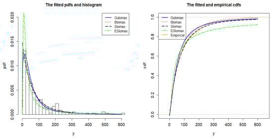
Figure 3. Fitted curves of the Gulomax, Blomax, ESlomax, and Slomax distribution.

Data 2: This dataset is about the lifespan of patients with heart failure and contains 96 patients with heart failure, the detailed information of which was provided by Tanvir Ahmad [27].

The numerical variables considered here are ejection fraction $\left(x_1\right)$, serum creatinine $\left(x_2\right)$, serum sodium $\left(x_3\right)$, and age $\left(x_4\right)$ as potential variables that explain cardiovascular mortality $\left(y\right)$. We apply the slashed Lomax regression model developed in Section 4 to this dataset. The resulting estimates and other regression models are given in Table 6.

Table 6. Parameter estimates and log-likelihood values for different models.

	Model
Parameter	RSlomax	RGulomax	RBlomax	RESlomax
$\alpha$	0.5340	5.2335	0.6819	0.6235
$\beta$	7.0880	7.6835	10.3537	-
$\lambda$	4.5721	8.6872	-	-
$\sigma$	-	3.8718	-	-
a	-	-	7.2867	5.8261
$\eta$	-	-	2.2743	-
${\gamma }_0$	−297.3180	−7.6412	1.1414	5.2382
${\gamma }_1$	0.1164	0.0142	0.0327	0.0688
${\gamma }_2$	−0.7148	0.2185	−0.4258	1.1429
${\gamma }_3$	2.1672	0.0843	−0.0259	0.0532
${\gamma }_4$	0.1286	−0.0820	−0.0674	−0.2133
-loglik	504.2635	508.7053	507.0078	526.2180
AIC	1024.5270	1035.4110	1032.0160	1066.4360
BIC	1045.0420	1058.4900	1055.0950	1084.3860

As can be noted from Table 6, the slashed Lomax regression model has the lowest AIC and BIC values among those of the other regression models. The values of these statistics indicate that the slashed Lomax regression model provides the best fit to the data. In addition, the increase of the content of serum creatinine will shorten the lifespan of patients and increase the risk of death, which are consistent with the conclusions by Tanvir Ahmad [27].

6. Discussion

In this article, the slashed Lomax distribution and its corresponding statistical properties are introduced. Maximum likelihood estimators through the ECM algorithm and simulation studies are discussed. In addition, the slashed Lomax regression model is studied. Applications to real data demonstrate the importance of the proposed distribution. In the future, we will consider extending this proposed model to the multivariate case and study its extremal properties, aiming to explore more practical values.

References

- Lomax, K.S. Business failures: Another example of the analysis of failure data. J. Am. Stat. Assoc. 1954, 49, 847–852. [Google Scholar] [CrossRef]
- Myhre, J.; Saunders, S. Screen testing and conditional probability of survival. Lect. Notes-Monogr. Ser. 1982, 2, 166–178. [Google Scholar]
- Balakrishnan, N.; Ahsanullah, M. Relations for single and product moments of record values from Lomax distribution. Sankhy Indian J. Stat. Ser. B 1994, 56, 140–146. [Google Scholar]
- Childs, A.; Balakrishnan, N.; Moshref, M. Order statistics from non-identical right-truncated Lomax random variables with applications. Stat. Pap. 2001, 42, 187–206. [Google Scholar] [CrossRef]
- Howlader, H.A.; Hossain, A.M. Bayesian survival estimation of Pareto distribution of the second kind based on failure-censored data. Comput. Stat. Data Anal. 2002, 38, 301–314. [Google Scholar] [CrossRef]
- Rogers, W.H.; Tukey, J.W. Understanding some long-tailed symmetrical distributions. Stat. Neerl. 1972, 26, 211–226. [Google Scholar] [CrossRef]
- Wang, J.; Genton, M.G. The multivariate skew slash distribution. J. Stat. Plan. Inference 2006, 136, 209–220. [Google Scholar] [CrossRef]
- Gómez, H.W.; Quintana, F.A.; Torres, F.J. A new family of slash-distributions with elliptical contours. Stat. Probab. Lett. 2007, 77, 717–725. [Google Scholar] [CrossRef]
- Arslan, O.; Genc, A.I. A generalization of the multivariate slash distribution. J. Stat. Plan. Inference 2009, 139, 1164–1170. [Google Scholar] [CrossRef]
- Reyes, J.; Gomez, H.W.; Bolfarine, H. Modified slash distribution. Statistics 2013, 47, 929–941. [Google Scholar] [CrossRef]
- Tian, W.; Wang, T.; Gupta, A.K. A new family of multivariate skew slash distribution. Commun. Stat. Theory Methods 2018, 47, 5812–5824. [Google Scholar] [CrossRef]
- Tian, W.; Han, G.; Wang, T.; Pipitpojanakarn, V. EM estimation for multivariate skew slash distribution. In Robustness in Econometrics; Springer: Cham, Switzerland, 2017; pp. 235–248. [Google Scholar]
- Gui, W. Statistical properties and applications of the Lindley slash distribution. J. Appl. Stat. Sci. 2012, 20, 283. [Google Scholar]
- Iriarte, Y.A.; Gomez, H.W.; Varela, H.; Bolfarine, H. Slashed rayleigh distribution. Rev. Colomb. Estadstica 2015, 38, 31–44. [Google Scholar] [CrossRef]
- Iriarte, Y.A.; Castillo, N.O.; Bolfarine, H.; Gomez, H.W. Modified slashed-Rayleigh distribution. Commun. Stat. Theory Methods 2018, 47, 3220–3233. [Google Scholar] [CrossRef]
- Reyes, J.; Vilca, F.; Gallardo, D.I.; Gomez, H.W. Modified slash Birnbaum–Saunders distribution. Hacet. J. Math. Stat. 2017, 46, 969–984. [Google Scholar] [CrossRef]
- Reyes, J.; Iriarte, Y.A.; Jodr, P.; Gomez, H.W. The Slash Lindley–Weibull Distribution. Methodol. Comput. Appl. Probab. 2019, 21, 235–251. [Google Scholar] [CrossRef]
- Iriarte, Y.A.; Rojas, M.A. Slashed power-Lindley distribution. Commun. Stat. Theory Methods 2019, 48, 1709–1720. [Google Scholar] [CrossRef]
- Astorga, J.M.; Iriarte, Y.A.; Gomez, H.W.; Bolfarine, H. Modified slashed generalized exponential distribution. Commun. Stat. Theory Methods 2019, 49, 4603–4617. [Google Scholar] [CrossRef]
- Gómez, Y.M.; Gallardo, D.I.; de Castro, M. A regression model for positive data based on the slashed half-normal distribution. Available online: https://www.ine.pt/revstat/pdf/Aregressionmodelforpositivedata.pdf (accessed on 1 January 2020).
- Jamal, F.; Reyad, H.M.; Nasir, M.A.; Chesneau, C.; Shah, M.A.A.; Ahmed, S.O. Topp-Leone Weibull-Lomax distribution: Properties, Regression Model and Applications. 2019. Available online: https://hal.archives-ouvertes.fr/hal-02270561/ (accessed on 1 January 2020).
- Hamedani, G.G.; Rasekhi, M.; Najibi, S.M.; Yousof, H.M.; Alizadeh, M. Type II general exponential class of distributions. Pak. J. Stat. Oper. Res. 2019, 15, 503–523. [Google Scholar] [CrossRef]
- Meng, X.L.; Rubin, D.B. Maximum likelihood estimation via the ECM algorithm: A general framework. Biometrika 1993, 80, 267–278. [Google Scholar] [CrossRef]
- Lemonte, A.J.; Cordeiro, G.M. An extended Lomax distribution. Statistics 2013, 47, 800–816. [Google Scholar] [CrossRef]
- Tahir, M.H.; Hussain, M.A.; Cordeiro, G.M.; Hamedani, G.G.; Mansoor, M.; Zubair, M. The Gumbel-Lomax distribution: Properties and applications. J. Stat. Theory Appl. 2016, 15, 61–79. [Google Scholar] [CrossRef]
- Kus, C. A new lifetime distribution. Comput. Stat. Data Anal. 2007, 51, 4497–4509. [Google Scholar] [CrossRef]
- Ahmad, T.; Munir, A.; Bhatti, S.H.; Aftab, M.; Raza, M.A. Survival analysis of heart failure patients: A case study. PLoS ONE 2017, 12, e0181001. [Google Scholar] [CrossRef] [PubMed]
Publisher’s Note: MDPI stays neutral with regard to jurisdictional claims in published maps and institutional affiliations. |
© 2020 by the authors. Licensee MDPI, Basel, Switzerland. This article is an open access article distributed under the terms and conditions of the Creative Commons Attribution (CC BY) license (http://creativecommons.org/licenses/by/4.0/).